conditions in real âwheel â railâ contacts are analyzed and friction coefficient is calculated as a ..... resulted in statistical scatter 3.4 % in the data, which support.
V.L. Popov, S.G. Psakhie, E.V. Shilko, et al. / Physical Mesomechanics 5 3 (2002) 1724
17
Friction coefficient in rail wheel-contacts as a function of material and loading parameters V.L. Popov1, 2, S.G. Psakhie2, E.V. Shilko2, A.I. Dmitriev2 K. Knothe3, F. Bucher3, and Ì. Ertz3 2
1 Padernborn University, Padernborn, D-33095, Germany Institute of Strength Physics and Materials Science, SB, RAS, Tomsk, 634021, Russia 3 Technical University of Berlin, Berlin, D-10623, Germany
Processes occurring in a surface layer of solids in friction are simulated by the method of movable cellular automata (MCA). The model considered accounts for elastic and plastic deformations as well as detaching and welding of wear particles. It is shown that relative movement of solids gives rise to a turbulent layer localized at the friction surface, in which intensive processes of mechanical mixing occur. We investigate the friction coefficient due to inelastic processes in the turbulent layer as a function of material parameters (yield stress, fracture stress, elastic moduli, viscosity, density) and loading parameters (sliding velocity and normal pressure). Numerical simulations show that the friction coefficient does depend only on two dimensionless combinations of the mentioned parameters. Loading conditions in real wheel rail contacts are analyzed and friction coefficient is calculated as a function of temperature.
I. Introduction The aim of the present work is to study the dependence of the coefficient of sliding friction in the wheel rail system on material and loading parameters. It is known that in a rolling contact of a body moving along a plane surface there are regions where there is no relative motion of bodies (stick regions) and regions where relative sliding takes place [1]. The law of sliding friction determines essentially the maximum force moment that can be transmitted through a wheel [2, 3]. It also defines the conditions for occurrence of instabilities in stationary rolling motion. On the one hand, the instabilities result in an increase in acoustic emission and noise level, and, on the other hand, can lead to macroscopic deformation of the rail and wheel (the so-called wheel polygonization) [24]. Thus, an investigation into the force of sliding friction as a function of loading and material parameters is of great importance for solving a number of topical technical problems of railway engineering. Generally speaking, friction is a process involving elastic interactions, plastic deformation, and failure processes at many scale levels. In this paper, we restrict ourselves to consideration of such tribological systems1 where solely 1 Under tribological systems we understand any systems including solids parts in relative movement, giving rise to friction and wear.
© V.L. Popov, S.G. Psakhie, E.V. Shilko, A.I. Dmitriev, K. Knothe, F. Bucher, and Ì. Ertz, 2002
elastic interactions among surface heterogeneities do not make a significant contribution to the friction force. As is shown in [5], this is the case if the so-called elastic correlation length of the system is much larger than the body size. This condition is almost always fulfilled for rigid bodies (e.g., made of materials with elastic moduli typical of metals) whose length of tribological contact is about a few centimeters. The absence of elastic contribution to the friction force implies that in the case where the bodies are absolutely elastic and absolutely smooth (in the sense of zero friction at the microlevel), the macroscopic friction force would be zero. This is due to the fact that elastic forces acting from micro-heterogeneities of one body on the microheterogeneities of the other are randomly directed; in the case of an absolutely rigid body (any body can be considered to be absolutely rigid whose size is smaller than the elastic correlation length), their averaging takes place and the macroscopic friction force is zero. The estimates show that in the case of the wheel rail system, the elastic correlation length far exceeds the length of the contact region (about 1 cm). The physical cause of friction forces for the foregoing contacts must, therefore, lie at a lower scale level and be due to the processes of inelastic deformation of surface volumes. To formulate an adequate model of friction processes in the wheel rail contact, it is necessary to determine a
V.L. Popov, S.G. Psakhie, E.V. Shilko, et al. / Physical Mesomechanics 5 3 (2002) 1724
2. Numerical model To model the processes in the surface layers, we use the method of movable cellular automata (MCA) [9, 10]. According to this method, a medium is represented as an ensemble of discrete elements movable cellular automata characterized by continuous variables such as center of mass position, value of plastic deformation, rotation pseudo-vector as well as by the discrete variables characterizing connectivity of the neighboring automata. The principles of writing the equation of motion for a system of cellular automata and prescribing interactions between them are described in [9].
In our case, a modeled object consisted of four parts (Fig. 1): the upper layer of automata was an absolutely rigid, nondeformable body moving horizontally at velocities v ranging between 1 and 10 m/s in different numerical experiments; two intermediate layers with initial roughness of nanometer range represented surface regions of the bodies in contact; the lower layer was a fixed support. A constant normal force corresponding to the pressure range between P = 0.5 MPa and P = 26 MPa acted upon all the elements of the upper layer. The diameter of the automata was from 2.5 to 10 nm in different numerical experiments. The elastic properties of the automata corresponded to the steel with Youngs modulus of E = 206 GPa and Poissons ratio of ν = 0.3. The yield strength σ y1 and ultimate strength with respect to tension σ0 were varied between 80 and 480 MPa and between 92 and 552 MPa, respectively. An important parameter determining stability of the plastic deformation processes and significantly affecting the characteristic size of the surface region of the severe plastic deformation is viscosity. Introduction of viscosity is necessary already from a formal consideration of providing stability to the calculation procedure. Phenomenological viscosity reflects dissipation processes under strain occurring due to electron and phonon excitation in a solid. It was assumed in the numerical model that viscous forces acting between unconnected but contacting automata are proportional to the relative velocity of motion. At the left and right fragment boundaries, periodic boundary conditions were used. The initial roughness was specified in the explicit form. The material parameters used are listed in Table 1 (for determination of strength parameters see Fig. 2). v = const P = const
Y
Thus, the railway wheel and rail surfaces show fractal structure in the wavelength range between 0.3 mm and 1 cm [7]. 1
In a pure elastic problem on the contact of fractal surfaces, the real contact area turns out to be zero, and the pressure in real contact regions to be infinitely high [8]. The real bodies, however, are not perfectly elastic and their contact region and maximum pressure at microcontacts depend on the hardness. The pressure at the microcontacts cannot significantly exceed the material hardness. This condition gives rise to contacts whose size is in the micrometer range.
55 nm
characteristic scale level where the processes responsible for the friction force formation occur. The surfaces of railway wheels and rails, as many other technical surfaces, have micro-heterogeneities at many scale levels; experimental studies show that these are self-similar surfaces in the wide range of surface scales and can be referred to the class of fractal ones1 [6, 7]. This suggests that both the size of the contact region and pressure distribution in the contact depend on the accuracy to which the surface micro-relief was determined. Thus, if we assume a model of absolutely smooth and elastic wheel and rail, we will have the solution first found by Hertz [1]. In view of fractal structure of surfaces, however, the real contact occurs in regions with sizes in the micrometer range2 [6, 7]. The transition to even lower (nanometer) scale level would cause further decrease in real contact area and increase in real pressure at nanocontacts. At this level, however, intense processes of plastic strain in materials take place. As pure elastic interactions on larger scales have been shown not to contribute substantially to the friction coefficient, we can conclude that it is the scale level at which the applicability of the theory of elasticity breaks down and intensive plastic deformation begins that determines the friction force in the systems under study. Based on the foregoing, we restrict our analysis to modeling the processes occurring at the submicrometer level. We consider a single contact with a typical size of about a few micrometers [6]. We distinguish such a small portion (with a linear size of about a hundred nanometers) from this microscopic region where the pressure is considered to be constant. The aim of the present paper is to study inelastic processes (plastic deformation and fracture) in this submicrometer ranges and to determine the friction forces resulting from these inelastic processes.
wheel
52.5 nm
18
rail
2
112.5 nm O
X
Fig. 1. Initial structure, dimension and loading conditions of the modeled fragment
19
V.L. Popov, S.G. Psakhie, E.V. Shilko, et al. / Physical Mesomechanics 5 3 (2002) 1724 Table 1 Parameters of a model material Young Modulus
E = 206 GPa
Poisson ratio
ν = 0.3
Density
ρ = 7 800 kg/m3
Elastic limit
σ y1 = 51306 MPA
Yield stress
σ y 2 = 80480 MPa
Strain at the yield stress
ε y 2 = 0.015
Tensile strength
σ 0 = 92552 MPa
Fracture deformation
ε c = 0.04
Viscosity
η = 0.41 Pa⋅s
Fig. 2. Definition of characteristic material parameters
3. Formation of a boundary quasiliquid layer The numerical experiments show that already within first nanoseconds after onset of a relative tangential motion of bodies, the roughness of both surfaces is severely deformed and fractured, and a dynamic equilibrium in the system is established at a temporal scale of about 100 ns. A pronounced boundary layer appears, where the processes of deformation, fracture, reconstruction of connectivity between elements, and intensive mixing take place. The motion in the layer resembles turbulent motion in liquid (Fig. 3). For this reason we refer to it as a quasi-liquid layer. Note, however, that this layer is not liquid in terms of thermodynamics. A quasi-liquid layer remains localized in the vicinity of the initial friction surface and does not propagate to deeper regions of the contacting bodies. A characteristic depth of the layer depends on the system parameters, first and foremost, on the effective viscosity of the system of automata. In our calculations, viscosity was used as a fitting parameter and was chosen so that the layer a
depth corresponded to the experimental values [10]. Particular form of the initial roughness does not influence the results of simulation. 4. Dependence of friction coefficient on loading and material parameters 4.1. Dependence on normal pressure Figure 4 shows a typical dependence of an average tangential force (friction force) on the applied normal pressure. In the series presented, the pressure took values of 1, 3, 5, 9, 15, 20, and 26 ÌPà at a constant value of sliding velocity of 5 m/s. To a first approximation, the force of friction increases in proportion to the normal pressure. Thus, the Amontons law [5] is approximately fulfilled. Note that the friction force at the beginning of motion is larger than the stationary value. Dynamics of friction coefficient can be important for the systems under study as the contact time of two micrometer-sized asperities can be comparable with the time of nonstationarity of the friction coefficient. A b
Fig. 3. Instant pictures of a quasi-liquid layer structure for a hypothetical material of ultimate strength σ 0 = 92 MPa: pressure P = 1 (a); 26 MPa (b). The slip velocity in both cases is 5 m/s. The zone of the quasi-liquid layer is shown by parenthesis
20
V.L. Popov, S.G. Psakhie, E.V. Shilko, et al. / Physical Mesomechanics 5 3 (2002) 1724
Fig. 4. Friction force versus pressure P in the runing-in stage (first hundred nanoseconds) and in the stationary state. The slip velocity is 5 m/s
Fig. 5. Friction coefficient versus velocity for pressure P = 15 MPa for a hypothetical material of an ultimate strength of σ 0 = 92 MPa
detailed study of transition processes is, however, beyond the scope of the present paper. Below we consider only the stationary value of the friction coefficient. The subject of our analysis is the study of a relatively weak dependence of the friction coefficient both on pressure and on other loading and material parameters. To study this dependence we performed 36 numerical experiments where all the parameters were varied (pressure, velocity, density, Youngs modulus, viscosity, and ultimate strength) except for Poissons ratio and the characteristic strains ε y 2 = 0.015 and ε c = 0.04. On varying the ultimate strength, the yield strength and limit of elasticity were changed in proportion to the ultimate strength.
follows that in the general case the friction coefficient may be thought of as a function of three independent combinations of the parameters2 ( E , σ 0 , ρ, v , P ). Empirical processing of the numerical experimental data shows, however, that the number of variables in the parameter region under study may be further reduced to two: it appears possible to present the friction coefficient (with an accuracy of 3.5 %) as a function of the following two dimensionless parameters:
4.1. Dependence on sliding velocity The velocity dependence of friction coefficient is of special interest from the standpoint of stability of tribological system. A typical dependence obtained in our numerical experiments for a normal pressure of 15 MPa is shown in Fig. 5. The increase in the friction coefficient with the velocity was recorded for other pressures as well. Note, however, that the coefficient of static friction was always higher than that of sliding friction. Thus, the friction coefficient first abruptly decreases and then monotonously increases with velocity. 4.2. Analytical approximation of friction coefficient Certain conclusions on the friction coefficient as a function of material and loading parameters can be made from the analysis of dimensionality. Indeed, the friction coefficient is a dimensionless quantity and, hence, can depend only on dimensionless combinations of system parameters. It can be shown that no dimensionless combination involving viscosity can be made up from material and loading parameters ( E , σ 0 , ρ, v , P, η). This implies that the friction coefficient cannot depend on viscosity1. The analysis of dimensionality shows that velocity v and density ρ can enter the relation for the friction coefficient only as ρv 2 . Hence it
κ1 =
ρv 2 E σ 02
and κ 2 =
PE . σ 02
(1)
Thus, changes in the parameters ( E , σ 0 , ρ, v , P, η) for constant κ1 and κ 2 in a set of 10 numerical experiments resulted in statistical scatter 3.4 % in the data, which support the hypothesis of dependence of the friction coefficient solely on parameters κ1 and κ 2 . Since we have no phenomenological model defining the form of the analytical dependence of the friction coefficient on loading parameters, we approximated the numerical data (34 points of numerical experiment) by the simplest rational function of the form µ = µ 0 + µ1
1 κ1 , + µ2 1 + bκ1 1 + cκ 2
(2)
that qualitatively reflects the main features of the soughtfor dependence. The least squares optimization gives the following numerical parameter values: µ 0 = 0.15, µ1 = 0.0442, µ 2 = 0.3243,
b = 0.195, c = 0.00212.
(3)
And thereby, on the quasi-liquid layer depth, which appears to be roughly proportional to viscosity. 1
Poissons ratio and fracture strain were kept constant in a set of numerical experiments used. Generally speaking, the friction coefficient can be also a function of these dimensionless parameters as independent variables. 2
V.L. Popov, S.G. Psakhie, E.V. Shilko, et al. / Physical Mesomechanics 5 3 (2002) 1724
21
a
0.6 0.5 0.4 20
0.3 10 500
κ2
300
100
0
κ1
0
Fig. 7. Friction coefficient versus dimensionless parameter κ 2 = PE σ 20 in the low velocity limit
b
As is shown later in the paper, the loading conditions at the rail wheel contact are such that parameter κ1 is often small and can be assumed to be zero. In this case, the friction coefficient can be represented as a function of parameter κ 2 alone: µ = µ0 +
or
µ2 1 + cκ 2
µ = 0.15 +
( κ1 → 0)
0.3243 . 1 + 0.00212 PE σ 02
(4) (5)
The dependence of the friction coefficient on parameter κ 2 determined by this relation is shown in Fig. 7. Fig. 6. Friction coefficient versus dimensionless parameters κ1 and κ 2 : analytical approximation (2) and simulation points (points beneath the surface are not shown) (a) and projection of the surface along the direction in which it is (almost) projected on the two-dimensional line (b). In this projection, a degree of scatter between calculation values and analytical data is shown (standard deviation 9 %)
5. Application to the rail wheel contact Let us estimate typical loading conditions in a tribological system rail wheel. Below, we distinguish three levels of consideration mentioned in the introduction: macrolevel, microasperity level, and nanolevel.
The approximation is accurate within 9 %. Dependence (2) is shown in Fig. 6(à). The degree of accuracy of approximation (2) can be assessed examining the surface shown in Fig. 6(a) and the points along the surface obtained from numerical experiments (projection in Fig. 6(b)). The numerical data suggest that the friction coefficient drastically decreases at very low pressures1. Construction of a unified analytical approximation for the entire pressure range is a complicated mathematical problem. For this reason, the points belonging to the low pressure range were not taken into account in constructing approximation (2). Therefore, the analytical dependence derived is applicable only for κ 2 ≥ 2.
5.1. Macrolevel At the macrolevel, we solve the problem of an elastic wheel rail contact, where the wheel and rail are considered to be perfectly elastic bodies bounded by smooth surfaces. The wheel rail contact region is known to have an elliptical form with the axis ratio of about a unit. For a typical load to the wheel of about 50100 kN and radius 0.5 m, the contact region diameter amounts up to 0.01 m (Hertzian contact). The maximum pressure is in the contact center and is about 500 MPa. For a rolling velocity of 50 m/s and characteristic wheel creep values from 2 to 10 %, we obtain typical slip rates in the contact region varying between 1 and 5 m/s.
This dependence is not physically unexpected: within P → 0, the friction coefficient must vanish. The friction coefficient, however, decreases in a narrow low-pressure range.
5.2. Asperity level To a second approximation, the fact that wheel and rail surfaces are rough is taken into account. A typical wave-
1
22
V.L. Popov, S.G. Psakhie, E.V. Shilko, et al. / Physical Mesomechanics 5 3 (2002) 1724 Table 2
a
Rail steel parameters as a function of temperature (according to manufacturers data) Temperature T, °C
20
200
300
400
600
Yield strength σ p 0.2 , MPa
510
533
528
408
244
Tensile strength σ m , MPa
922
877
978
875
409
Fracture deformation ε, %
10.4
6.65
6.11
16.07
24.5
b
length of a surface asperity is about 10 µm, and height 0.1 µm. The calculation of real contact surface and pressure at microcontacts made for the contacts with experimentally measured roughness [3, 6] show that the contact area ranges from 0.2 to 0.5 of the nominal contact area. The maximum pressures at contacts at the microlevel vary between 1 000 and 2 500 MPa. Note that the latter value corresponds to rail steel hardness (about 3σ 0 [13]). This suggests that consideration of a problem on elastic deformation at the level of ever smaller heterogeneities has no physical meaning, since it is at this low level (submicrometer level) where severe plastic deformation processes occur. It is for this reason that we continue further motion in the direction to the submicrolevel in terms of a dynamical model based on movable cellular automata. In doing so, pressure and velocities obtained at the microlevel serve as boundary conditions for a nanoscale-level problem.
5.3. Nanoscale level The foregoing estimates of pressure at microcontacts in combination with elastic and strength characteristics of rail steel used by the Deutsche Bahn AG (Table 2), show that the dimensionless variables κ1 and κ 2 take values from the following ranges: κ1 = 0 K 0.25, κ 2 = 0 K1533.
(6)
Thus for real contacts, κ1 is small and to a first approximation may be considered to be zero. Therefore, approximations (4) and (5) can be used to study the wheel rail contacts. Note that both the theoretical analysis and direct numerical calculations show that the probability distribution to find a specified pressure at a contact between two fractal surfaces becomes the more uniform, the lower the scale level [7, 8]. Thus, at the scale level where the peak pressure achieve hardness of the material, the probability distribution has the form shown in Fig. 8. Considering, to a first approximation, the pressure distribution to be uniform in the range from 0 to hardness 3σ 0 , we can average dependence (5) to get
c
Fig. 8. Distribution function of probability P(σ, ζ) to find a specified pressure σ at the rail wheel rail contact with real (experimentally measured) roughness (data from [6]). The distribution function depends on the wavelength λ at which the Fourier spectrum of the surface profile is cutoff in order to solve the elastic contact problem. The ratio of the apparent contact size to the cut-off wavelength is the scaling parameter ζ (the value ζ = 1 corresponds to the assumption of absolutely flat contact). Three distributions shown correspond to the spectrum cutoff at wavelengths 1, 0.01, and 0.025 cm, respectively. The finer the asperities taken into account the higher the peak pressure values achieved at the contacts, and the more uniform the probability distribution in the moderate pressure range. The lower picture shows pressure distribution at the sub-micrometer level examined in this work. To a first approximation, the probability distribution in this case can be considered to be uniform in the range from zero to hardness of the material
µ=
3σ 0
3σ 0
0
0
∫
Pµ( P ) dP
∫ P dP .
(7)
The integral in the numerator determines the total friction force, and that in the denominator the total force of normal pressure; their ratio is the friction coefficient observed at the macrolevel. Thus defined macroscopic friction coefficient is independent of pressure:
23
V.L. Popov, S.G. Psakhie, E.V. Shilko, et al. / Physical Mesomechanics 5 3 (2002) 1724
Fig. 9. Tensile strength σ 0 of rail steel versus absolute temperature
µ = 0.15 + 1020
2
σ0 σ − 2 ⋅107 0 − E E
(8)
2
E σ . − 1.6 ⋅ 10 6 0 ln 2.5 ⋅ 105 + 159 σ 0 E Note that the dependence of the friction coefficient on the velocity is given by a simple additive (independent of pressure) term, according to Eq. (2). Hence the resulting dependence of the friction coefficient on the material parameters and slip velocity under the assumption that the pressures are evenly distributed can be written as follows:
µ = 0.15 + 1020
2
σ0 σ − 2 ⋅107 0 − E E 2
E σ − 1.6 ⋅ 10 6 0 ln 2.5 ⋅ 105 + 159 E σ 0 + 0.0442
ρv 2 E σ 02
1 + 0.195 ρv 2 E σ 02
+
(9)
.
If the assumption on even pressure distribution is not valid, a more general Eq. (5) should be used. 5.4. Temperature dependence of the friction coefficient The friction coefficient of the system under study does not depend explicitly on temperature T. Temperature can, therefore, influence the friction coefficient only by the temperature dependence of mechanical parameters. Let us analyze averaged friction coefficient (9). It does not depend on pressure. As noted above, it is also practically independent of velocity and is a function of the strength to Youngs modulus ratio σ 0 E in the wheel rail system. The friction coefficient can be changed only due to changes in these values caused by temperature variations. Ultimate strength of a material is most heavily temperature-dependent. Let us use the data on temperature ultimate strength depen-
Fig. 10. Theoretical dependence of the rail steel friction coefficient on absolute temperature
dence summarized in Table 2. Assuming that the decrease in strength at increased temperatures is due to heat-activated plastic deformation processes, the experimental data can be approximated by the following dependence: σ1 , T ≤ T0 , σ0 = U0 T + ξT ln ψe
(ψe ) + 1 , T > T , U0 T 2
0
(10)
with σ1 = 925.7, T0 = 663, U 0 = 3 074, ξ = 5.936, and ψ = = 0.0023. Dependence (10) for the given parameter values and experimental points are shown in Fig. 9. Substituting Eq. (10) in Eq. (8), we derive the temperature dependence of the rail steel friction coefficient shown in Fig. 10. In the temperature range up to 700 K, the friction coefficient is independent of temperature. But it drastically decreases as the temperature increases to 1 000 Ê and more. What is the probability that such temperatures will be achieved in microcontacts? First of all, we should distinguish between the average temperature occurring at a Hertzian contact for a single wheel roll and peak microcontact temperatures. As is shown in [12], the increase in the average temperature at the contact does not exceed 150 K, and thus the absolute temperature reaches 450 K at maximum. This suggests that temperature cannot considerably alter the friction coefficient. However, peak temperatures at microcontacts can achieve much higher values (about 1 000 K) and significantly affect the friction coefficient [13]. A quantitative evaluation of this effect would require a self-consistent solution to the problem on heat release and propagation in the microcontacts, with the friction coefficient being determined by complete equation (2). Averaging method (7), and thus equations (8) and (9) based on it are not applicable in this case. A solution to the relevant self-consistent problem is beyond the scope of this work.
24
V.L. Popov, S.G. Psakhie, E.V. Shilko, et al. / Physical Mesomechanics 5 3 (2002) 1724
6. Concluding remarks The major result of this work is expressed by Eq. (2) determining the dependence of the friction coefficient at the submicrolevel on two dimensionless arguments. These arguments, in turn, depend on the material (density, strength, and Youngs modulus) and loading (pressure and slip velocity) parameters. We have found that the friction coefficient depends strongly on the dynamic processes in surface nanolayers that are formed and sustained at the contact region within the entire period of relative motion of contacting solids. The fact that the friction coefficient depends only on two independent arguments κ1 and κ 2 (1) does not follow from the analysis of dimensionality and has come as an unexpected empirical fact requiring theoretical interpretation. It should be noted that dependence (2) was found for a number of simplifying assumptions. The major assumptions are: Equation (2) is valid only within 2 ≤ κ 2 ≤ 1800. The lower limit of this range gives the minimum values of κ 2 used for deriving approximation (2), and the higher limit determines the studied range of κ 2 values (note, however, that for κ 2 = 1 800 there was only one calculation; the most completely studied region is for κ 2 ≤ 620). Poissons ratio was taken to be 0.3, and breaking strain under active loading 4 %. These values are typical of many metals. In contrast, higher values of Poissons ratio and breaking strain are typical of polymers and, in particular, rubber. Tribological systems whose linear dimension is much smaller than the elastic correlation length were examined. This assumption is reasonably well fulfilled for contacts of interest with dimension of about 1 cm in the case of metals, and is not fulfilled in the case of rubber-like soft materials. The contacting materials were assumed to be homogeneous. Hence all elements of the medium and their strength and elastic characteristics were identical. Evidently, this assumption is not fulfilled for many alloys and steels. We suggest that due to the presence of a dynamic boundary layer, the effect of structural heterogeneities is averaged. However, further investigation into the subject is required. Another important result is concerned with a macroscopic friction coefficient observed at the contact of surfaces with a random (fractal) roughness. We brought forward arguments in support of the fact that in this case, the probability of finding a specified pressure at the contact is (approximately) uniformly distributed in the range from zero to hard-
ness of material (on the order of magnitude equal to thrice the strength relative to that at uniaxial strain). Averaging the friction coefficient over this distribution gives the friction coefficient depending on the material strength to Youngs modulus ratio σ 0 E and κ1 = ρv 2 E σ 02 alone. However, these conclusions are correct only in the case where temperature effects at microcontacts are ignored. Undoubtedly, a general qualitative conclusion is the fact that dynamic processes of plastic deformation and fracture at the nanolevel are of great importance. To our mind, these processes are the key to investigation into friction mechanisms in real tribological systems. Acknowledgements One of the authors (V.L. Popov) is grateful to O. Dudko for discussions and comments. Financial support from the Deutsche Forschungsgemeinschaft in the frame of the SFB 605 and the German Academic Exchange Service (DAAD) is acknowledged. References [1] K.L. Johnson, Contact Mechanics, Cambridge University Press, 1985. [2] J.B. Nielsen, Evolution of rail corrugation predicted with a non-linear wear model, J. Sound and Vibration, 227, No. 5 (1999) 915 [3] K. Knothe, R. Wille, and B.W. Zastrau, Advanced contact mechanics road and rail, Vehicle Systems Dynamics, 35, Nos. 45 (2001) 361. [4] V.L. Popov and A.V. Kolubaev, Generation of surface waves during external friction of elastic solid bodies, Tech. Phys. Lett., 21. No. 10 (1995) 812. [5] B.N.J. Persson, Sliding Friction. Physical Principles and Applications, Springer Verlag, New York, 2000. [6] F. Bucher, K. Knothe, and A. Theiler, Normal and tangential contact problem of surfaces with measured roughness (2002) (to appear in Wear). [7] B.N.J. Persson, F. Bucher, and B. Chiaia, Elastic Contact Between Randomly Rough Surfaces: Comparison of Theory with (Exact) Numerical Results (2001) (to appear in J. Chem. Phys.). [8] B.N.J. Persson, Elastoplastic Contact between Randomly Rough Surfaces, Phys. Rev. Lett., 87, No. 11 (2001) 116101. [9] V.L. Popov and S.G. Psakhie, Theoretical principles of modeling elastoplastic media by movable cellular automata method. I. Homogeneous media, Phys. Mesomech., 4, No. 1 (2001) 15. [10] V.L. Popov, S.G. Psakhie, A. Gerve, B. Kehrwald, E.V. Shilko, and A.I. Dmitriev, Wear in combustion engines: experiment and simulation on a basis of movable cellular automaton method, Phys. Mesomech., 4, No. 4 (2001) 71. [11] A.H. Cottrell, The Mechanical Properties of Matter, John Wiley & Sons, New York, 1964. [12] M. Ertz and K. Knothe, Einfluss von Temperatur und Rauheit auf den Kraftschluss zwischen Rad und Schiene, ZAMM, 81 (2001) 57. [13] V.L. Popov, V. Rubzov, and A.V. Kolubaev, Blitztemperaturen bei Reibung in hoch belasteten Reibungspaaren, Tribologie und Schmierungstechnik, 6 (2000) 35.