Feb 7, 2013 - devices and many others cause mechanical anisotropy due to different friction or/and .... column, stiff protuberances on a stiff supporting layer.
SUBJECT AREAS: BIOMECHANICS COMPUTATIONAL BIOPHYSICS BIOINSPIRED MATERIALS
Frictional-anisotropy-based systems in biology: structural diversity and numerical model Alexander Filippov1 & Stanislav N. Gorb2
MECHANICAL PROPERTIES 1
Donetsk Institute for Physics and Engineering, National Academy of Science, Donetsk, Ukraine, 2Department of Functional Morphology and Biomechanics, Zoological Institute of the Kiel University, Am Botanischen Garten 1–9, D-24098 Kiel, Germany.
Received 29 October 2012 Accepted 10 January 2013 Published 7 February 2013
Correspondence and requests for materials should be addressed to S.N.G. (sgorb@ zoologie.uni-kiel.de)
There is a huge variety in biological surfaces covered with micro- and nanostructures oriented at some angle to the supporting surface. Such structures, for example snake skin, burr-covered plant leaves, cleaning devices and many others cause mechanical anisotropy due to different friction or/and mechanical interlocking during sliding in contact with another surface in different directions. Such surfaces serve propulsion generation on the substrate (or within the substrate) for the purpose of locomotion or for transporting items. We have theoretically studied the dependence of anisotropic friction efficiency in these systems on (1) the slope of the surface structures, (2) rigidity of their joints, and (3) sliding speed. Based on the proposed model, we suggest the generalized optimal set of variables for maximizing functional efficiency of anisotropic systems of this type. Finally, we discuss the optimal set of such parameters from the perspective of biological systems.
A
nisotropic surfaces are widespread in the non-biological world ranging from the molecular level1 to the macroscopic level. The crystal structure of solids leads to the anisotropy of their surfaces on an atomic level. In engineering, anisotropy of certain texture patterns of polycrystalline materials is produced naturally or artificially during manufacturing of the materials. Surface anisotropy manifests itself even on geological scales where, due to tectonics, a majority of structures have well developed anisotropy. There is also a huge variety in biological surfaces covered with micro- and nanostructures oriented at some angle to the supporting surface2–4. Such structures cause mechanical anisotropy due to different friction or/and mechanical interlocking during sliding in contact with another surface in different directions. Such surfaces serve propulsion generation on the substrate (or within the substrate) for the purpose of locomotion or for transporting items. They have been previously described in a variety of mechanical systems belonging to different organisms ranging from the insect unguitractor plate5–9, interlocking mechanisms of joints in insect legs and antennae3, insect ovipositor valvulae3,10–13, animal attachment pads14–19, inner surface of pitcher plants20–22, wheat awns23, fluids-guiding systems of plants24, butterfly wings25, etc. The surface outgrowths, their joints to the supporting layer, and the supporting layer itself in most anisotropic surfaces in biology are rather rigid and rely on the ratchet principle in their mechanical behavior. However, some systems exhibit pronounced flexibility of surface structures due to the flexible material of the supporting layer or due to a specialized flexible joint connecting to the rigid supporting layer. A typical macroscale system of this kind is the snake skin consisting of rather stiff scales26 embedded in a rather flexible supporting layer (Fig. 1). Preferred orientation of both scales themselves and surface microstructures has been discussed to be the key features responsible for the frictional anisotropy in this particular system27–30 (Fig. 2F). In addition, there is a microstructure at the level of the scale with strongly anisotropic orientation, which has been recently demonstrated to provide frictional anisotropy of the snake skin29,40 (Fig. 2G). Also shark skin exhibits a similar arrangement of stiff surface denticles embedded in a flexible collagenous supportive layer31. Another example has been reported from the burr-covered Galium aparine plant leaves/stems/fruits32, where burrs are connected to the supporting layer with a flexible joint33. Cleaning devices of insects consist of rigid setae connected to the surface also with flexible joints34–36 (Fig. 3). These numerous examples have a wide range of functions from the transport of particles (cleaning devices), the leaf positioning on the top of another leaf to the propulsion generation during slithering locomotion (snake). Since the rigidity of the support must have an influence on the mechanical behavior of these systems (as recently was shown for the snake skin40), we have developed, in this paper, a model aiming at the study of their mechanical
SCIENTIFIC REPORTS | 3 : 1240 | DOI: 10.1038/srep01240
1
www.nature.com/scientificreports
Figure 1 | Diagram of ratchet-like frictional anisotropic systems. First column, stiff protuberances on a stiff supporting layer. Second column, soft protuberances on a stiff supporting layer. Third column, stiff protuberances on a soft supporting layer. The third (framed) column indicates the system considered in the present study. First row, systems in non-deformed state. Second row, deformation caused by sliding in the direction of the protuberance slope. Third row, deformation caused by sliding in the direction opposite to the protuberance slope.
behavior (Fig. 4). We studied the dependence of the anisotropic friction efficiency on (1) the slope of the surface structures, (2) rigidity of their joints, and (3) sliding speed. Based on the proposed model, we suggest the generalized optimal set of variables for maximizing functional efficiency of anisotropic systems of this type. Finally, we discuss the optimal combination of such parameters from the perspective of biological systems.
Results Typical time-dependencies of the friction force Ffriction (t) at positive V . 0 and negative V , 0 velocities are presented in the subplots (a) and (b) of Fig. 5, respectively. Bold lines in both cases show mean friction force ðt 1 vFfriction w~ Ffriction (t), ð2Þ t t~0
Figure 2 | System that assists body propulsion for locomotion. (A–E). Diagram showing how the soft-embedded sloped stiff array of protuberances can generate propulsion due to the opposite movements along a non-smooth substrate. (F, G). Lateral scales of the snake Python regius at different magnifications in the scanning electron microscope (SEM). d, direction toward the tail (caudal); DT, denticulations; SC, scales. SCIENTIFIC REPORTS | 3 : 1240 | DOI: 10.1038/srep01240
Figure 3 | System that generates particle movement for cleaning. (A–E). Diagram showing how the soft-embedded sloped stiff array of protuberances can generate unidirectional particle motion due to opposite movements along a substrate. (F, G). Foreleg of the ant Formica polyctena with a specialized cleaning device at different magnifications in SEM. d, distal direction; ST, setae.
accumulated from starting moment t 5 0 to a current time t. Mean force vFfriction w averaged during sufficiently long time runs can be used to characterize the difference in system properties at varied elasticity Kb and velocities V. Results of numerical simulations performed at V~+1 and varied Kb are presented in Fig. 6, where vFfriction w is shown in an interval of a few orders of amplitude 10{3 ƒKb v104 . A wide interval of Kb , where the system demonstrates strong anisotropy of the friction, is clearly seen. The optimal value of Kb is marked by a dash-dotted line. At a given set of the parameters it is around Kb ^1. It is important to note that the model is robust against particular choice of the elastic force felastic (b). This force was chosen above as the linear function felastic ~Kb (b0 {b), partially because we believe that this force monotonously increases with the deviation of the angle b0 {b from its equilibrium value, partially because to the moment we do not know its correct real dependence. An alternative choice could be felastic ~Kb sin (b0 {b) which reflects the fact that distortions of the skindl* cos (b0 {b) which tends as effective springs prevent a rotation of the fibers is proportional to the cosine: dl* cos (b0 {b). Corresponding force felastic ~Kb sin (b0 {b) degenerates into linear one felastic ~Kb (b0 {b) at small deviations (b0 {b)?0. The results obtained in this variant of the model must coincide with the linear one in this limit. Stronger difference is expected in principle for large deviations, which can appear at negative velocitiesVv0 and weak elastic constant Kb =1, when external force is able to rotate fibers strongly. However, in this limit felastic ~Kb sin (b0 {b) also becomes nonrealistic too, because the force felastic must grow monotonously at large deviations. To compare two variants of the model, we performed numerical simulations with felastic ~Kb sin (b0 {b) also. The results are shown in Fig. 6 by dotted curve. As expected, a deviation is observable only for a combination of negative velocity Vv0 and weak elastic constant Kb =1. For stronger Kb §1and for all positive velocities Vw0 two variants almost perfectly coincide (for positive V the difference is practically invisible in the figure). Let us account also, that majority of the results below will be obtained for the elastic constant close to the optimal value Kb ^1. It allows limiting ourselves by the simplest linear model felastic ~Kb (b0 {b). It is also important to admit that the present basic minimalistic model leaves outside the consideration of many important parameters, such as density and geometry of the stiff fibers, their length, thickness, etc, which may also affect the results. All these questions remain open for more specific further studies of 2
www.nature.com/scientificreports
Figure 4 | Conceptual diagram of the model. The motion of the system is determined by Eq. (1) at equal damping constants c~cb ~1, fixed elasticity K~1of external spring and interaction f0 ~1between the probe and hairs. Two other parameters: external velocity Vand rigidity against rotations Kb remain varied.
concrete biological systems. The main advantage of the present model is in its simplicity and transparency both allowing considering the importance of the flexibility of structures for tuning of frictional anisotropy. It is interesting also to study the inverse problem and apply friction anisotropy (which is, in fact, caused by real anisotropy of the interaction between the substrate and probe) to produce a directed drift of a ‘‘cargo’’. To do this, let us put the probe on the top of the substrate and perform periodic oscillations of the substrate. One can check numerically that anisotropy of interaction really leads to a directed motion. We found directed drift even when a gently colored random noise of fluctuations with slightly preferable frequency V instead of strictly periodic oscillations is applied. Such sustainability against perturbations, and even ability of the system to produce directed motion at weakly pronounced preferences, must be extremely important for the biological applications of the effect. However, for the goals of this paper, below we limit ourselves to the strictly periodic oscillations with unique frequency V. The numerical experiment in this case is as follows. We use the same Eq.(1), but change the external force to zero K(Vt{x)~0. Instead, we move the substrate periodically and find out how the probe position changes during a sufficiently long run. Appearance of
the directed drift is characterized by a non-zero mean velocity vVx w: ðt 1 Vx (t)=0 ð3Þ vVx w~ t t~0
Figure 7 shows a dependence of mean drift velocity vVx w on the Kb elastic constant at some representative frequencies V. The larger vVx w, the more pronounced the effect appears. Dot-dashed line in the figure corresponds to the optimal elasticity Kb ^1. At high frequencies curves vVx wstart to shift down monotonously. We do not show directly all the curves in order not to overload the figure. Instead, the direction of the shift is qualitatively marked by an arrow. One can collect optimal values of the drift velocity, found on each curve near Kb ^1, and plot them as a function of V. This is done in Fig. 8. Starting from a frequency slightly higher than V~0:5(around V~2p=10 shown in Fig. 7) marked by a dash-dotted line, the drift exponentially goes down, especially at V??. This exponential decay is clearly confirmed by the logarithmic plot in the insert to Fig. 8. At low frequencies Vƒ0:5 drift velocity is almost constant. It means that at small frequencies Vƒ0:5 the probe always has enough time to be captured by the substrate motion and tends to move much
Figure 5 | Typical time dependencies of the friction force for positive Vw0(a) and negative Vv0 (b) velocities. Bold lines in both cases show mean friction force (Ffriction) averaged starting from t~0 to a current moment of time t. The parameters are the same as in Fig. 4. SCIENTIFIC REPORTS | 3 : 1240 | DOI: 10.1038/srep01240
3
www.nature.com/scientificreports
Figure 6 | Mean friction forces for fixed positive and negative velocities V~+1 accumulated for a few orders of the absolute value 10{3 ƒKb v104 . Optimal elasticity around at Kb