From AADL architectural models to Petri Nets : Checking model viability∗ Xavier R ENAULT, Fabrice KORDON Universit´e Pierre & Marie Curie, Laboratoire d’Informatique de Paris 6/MoVe 4, place Jussieu, F-75252 Paris CEDEX 05
[email protected],
[email protected]
Abstract Modeling of Distributed Real-Time Embedded (DRE) systems allows one to evaluate models behavior or schedulability. However, assessing that a DRE system’s behavior is correct in the causal domain is a challenge: one need to elaborate a mathematical abstraction suitable for checking properties like absence of deadlock or safety conditions (i.e. an invariant remains all over the execution). In this paper, we propose a global approach to building Petri Nets models from an architecture described using AADL. We consider the semantics of interacting entities defined by AADL, and show how to build corresponding Petri Nets models. Based on a case study, we show how the verification process could be automated and parameterized.
1. Introduction Complexity of current real-time systems, in both the embedded and critical domains, call for new methods, processes and tools. Model Driven Development approaches are of interest because they focus on a consistent description of systems, their functional and non-functional properties. However, building multiple views of the same systems, with potentially several formal notations is not an affordable solution, as it increases the number of artifacts to be maintained and updated. Dedicated modeling frameworks like MARTE [12] and AADL [14] provide a high-level formalism to describe a system, at both the functional and nonfunctional levels. Tools exist to provide simple analysis like Rate Monotonic Scheduling (RMA), but none of them address the more complex challenge of testing or verifying the behavior of a complete system. ∗ This
work has been funded in part by the ANR Flex-eWare project
J´erˆome H UGUES, Institut TELECOM, TELECOM ParisTech, LTCI 46, rue Barrault, F-75634 Paris CEDEX 13
[email protected]
When involved notations are formal, it is possible to reason on the specification to check properties (from validation to verification). In-depth analysis of their behavior, i.e. causality analysis of a system then becomes possible. However, the modeling and verification process remains difficult to handle by engineers. There is a need to rely on high-level notations such as MARTE or AADL. MARTE provides a generic canvas to describe and analyze systems. This genericity requires the user needs to add specific modeling artifacts to model the semantics of the selected runtime (such as POSIX [2]) or uses an existing profile specified as part of MARTE, like the AADL profile. Compared to MARTE, the AADL language comes stand-alone with a complete semantics, defined and enforced by a standard. This semi-formal semantics is defined as hybrid automata to express thread’s behavior, and invariants for dispatching, and communication time. In this paper, we propose to bridge AADL specifications with Petri Nets. This formal notation is well-suited to describe behaviors of concurrent systems and provide good formal analysis capabilities [5] such as structural analysis and model checking. The objective is to check that AADL models are deadlock-free, livelock-free and bounded (i.e. no buffer needs to be of infinite size). Section 2 briefly presents Petri Nets and AADL. Then, section3 describes the patterns ensuring correspondence between AADL and Petri Nets semantics. Section 4 illustrates the use of these pattern on an example and show what type of analysis can be performed on an AADL model.
2. Petri Net patterns For AADL 2.1
Introduction to Symmetric Nets
This section provides an informal presentation of Symmetric Nets. Formal definitions can be found in [1, 5].
Symmetric Nets are Colored Petri Nets enhanced with highlevel features: tokens can carry data. Therefore, a data type is associated with each place, indicating the data type of the tokens in that place. Only simple data and manipulation functions are permitted, allowing for powerful analysis techniques: finite enumerated types, intervals, tuples; and the basic functions: predecessor, successor, selector (in a tuple) and “broadcast” (generates one copy of each possible value of a data type). An example is shown in Figure 1. It represents two threads asynchronously communicating by means of events. Places Ready and Halted correspond to the event producer while places Wait and Done describe event managers’ behavior. Marking indicates there are three threads able to handle events. The number of event generator threads (initial marking M in Ready) depends on constant Q. Events are distinguished thanks to Queries’ id (value in color class Query). Here, we represent the signal queue by means of a place but a complete Queue design pattern [10] can be used to reflect additional information on the system behavior. Ready M M=+...+
Class Query Query is 1..Q; Var GenQuery q in Query; Signal Query Halted Query
• Wait •• GetQuery Done Query
Figure 1. Example of a Symmetric Net. From this model, one can generate all possible actions. For example, the state space generated for Q = 5 (i.e. 5 requests) contains 232 nodes and 760 arcs and outline 10 possible deadlocks. None of them corresponds to the terminal state of such a system where all tokens are in places Halted and Done. This is due to the lack of tokens in place Wait: the number of event handlers is not sufficient to process all events. This specification can easily be corrected by initially putting Q tokens in Wait. Petri Nets allow for structural analysis (i.e. computation of properties without computing the system’s state space). For example, computation of structural bounds show that place Signal may contain at most Q tokens. Thus, dimensioning of the system can be formally verified.
2.2
Introduction to AADL
AADL is an architecture description language, standardized by the SAE. It has been specifically designed for DRE systems. AADL is component-centric and allows the modeling of both software and hardware parts of DRE systems. It focuses on the definition of consistent block interfaces,
and separates implementation from interfaces. Both graphical and textual syntaxes are defined in the standard. The behavior of a system, e.g. how functional blocks interact, is fully defined in the standard by mean of dispatching invariants, communication patterns. It is configured by the set of non-functional properties applied to each model element. Non-functional aspects of components can be described within an AADL model such as thread dispatching condition (periodic or sporadic), interface specifications and how components are interconnected. These have a deep impact on the system’s behavior. Functional aspects (algorithmic/behavioral specifications) are attached separately as source code by means of AADL properties. A model is made of components. The AADL distinguishes: software components (data, thread, thread group, subprogram, process), execution platform components (memory, bus, processor, device) and hybrid components (system). Components describe elements of the actual architecture. Systems are bounding blocks to help structure the description. Subprograms model procedures. Threads model the active part of an application (e.g. POSIX threads). AADL threads may have multiple operational modes. Each mode may describe a different behavior and property values for the thread. Processes are memory spaces that contain the threads. Thread groups are used to create a hierarchy among threads. Processors model processors and the OS scheduler. Memories model storage, buses support communication, devices are general hardware. Components may be hierarchical, i.e.: components can contain other components (called subcomponents in this case). In fact, an AADL description is always hierarchical, with the topmost component being an AADL system that contains—for example—processes and processors, with the processes containing threads and data, and so on. The interface specification of a component is called its type. It provides features (e.g. communication ports). Components communicate one with another by connecting their features. To a given component type correspond zero or more implementations. Each of them describes the internals of the component: subcomponents, connections between these subcomponents, etc. An implementation of a thread or a subprogram can specify call sequences to other subprograms, thus describing the execution flows in the architecture. Since there can be different implementations of a given component type, it is possible to select the actual components to be put into the architecture, without having to change the other components, thus providing a convenient approach to application configuration. AADL defines the notion of properties that can be attached to most elements (components, connections, features etc.). Properties are name/value pairs that specify constraints or characteristics that apply to the elements of the
Thread life cycle b c
•
d
performingThreadInitialization h suspendedAvaitingMode i k
a Error management threadHalted f
e1
e2
a
threadHalted
e3
e4
performingThreadDeactivation
f performingThreadInitialization
d
e5
h c
j
j
k performingThreadDeactivation
o
Thread execution
Complete
performingThreadActivation
m
n
performingThreadFinalize l
o b
AwaitDispatch performingThreadComputation
e1
suspendedAvaitingMode
i
performingThreadFinalize performingThreadActivation l suspendedAwaitingDispatch
m
AwaitDispatch
n
e2 e4 e3
suspendedAwaitingDispatch
Complete
performingThreadComputation
e5
Figure 2. Petri Net derived from the AADL thread automata and its associated state space architecture: frequency of a processor, execution time of a thread, bandwidth of a bus, etc. Some standard properties are defined; but it is possible to define one’s own properties. A detailed introduction to AADL can be found in [3]. AADL provides two major benefits for building DRE systems. First, compared to other modeling languages, AADL defines low-level abstractions including hardware descriptions. These abstractions are more likely to help designing a full system, close to the final product. Second, the hybrid system components help refine the architecture as they can be detailed later on during the design process, allowing for different stages of modeling, from early requirements down to executable models. Different analysis exist for AADL: schedulability [15], error modeling [4], but also code generation [9]. In this paper, we focus on the behavioral analysis of Petri Net models, as an application of our approach.
3
From AADL to Symmetric Net
This section is dedicated to the definition of patterns handling transformation of AADL into Petri Nets that handle verification of complex systems like a middleware in [8]. We aim at qualitative analysis of AADL specifications. Therefore, we selected Symmetric Nets [5]. They are suitable for a deep analysis of causal property in distributed systems. This enables verification of safety properties (e.g. a dangerous states of a system cannot be reached) and requires a deeper modeling of AADL patterns, compared for instance to stochastic analysis ([13]), or timed verification.
3.1
AADL Thread Automata
In AADL, behavior is mostly represented by Threads Components and their interactions through “features”:
event or data ports. These interactions are thus represented by communication places in the Petri Net to trigger associated actions when AADL threads receive new data (Petri Net tokens). Other components type like system, processes simply define bounding boxes. Figure 2 shows the Petri Net modeling the AADL thread automata defined in the standard1 (left) and the associated state space (right). Guards of the standard are discarded: we only specify the possibility of any event to occur. This model is the main pattern to which sub-Petri patterns describing local behavioral descriptions are connected. With one token in threadHalted (i.e. the initial state of an AADL thread), we produce a state space equivalent to the original automata depicted in the standard as shown in figure 2. It reaches the same states for the same input events, showing equivalence between both models (the automata from the standard is not presented here due to space concerns but it has exactly the same structure, which is not surprising considered the translation schema). This automata is divided in three parts: i) the Thread life cycle that handles dispatching, initialization and completion, ii) the Thread execution that corresponds to the execution of computation-defined code and, iii) the Error management that handles potential errors during the execution. Transitions Complete and AwaitDispatch are interfaces of both Thread life cycle and Thread execution of the automata. Transformation rules presented in this section generates sub-Petri Nets that are connected to these transitions. To cope with the AADL namespace concept, we prefix Petri Net elements with the identifier of the enclosing AADL entity (e.g. process,thread). This ensures traceability of elements. This is important to provide relevant diagnostics after analysis of generated Petri Nets. 1 Figure
5 of section 5.4.1 in [14].
3.2
Transformation Rules
We now detail the transformation rules generating subPetri Nets connected to the model of Figure 2. As some rules are parameterized, we first define the following types: • T hT ypei denotes a hT ypei-typed element, e.g. T AADL P ort defines an AADL Port Type; • L hT ypei denotes a list of hT ypei-typed elements; • L T AADL hT ypei gethT ypei (T AADL System) returns all hT ypei-entities of a given system In AADL, port contains the following informations: T Direction to distinguish between an input or an output port and T Kind for data, event or event data port. 3.2.1
Main Transformation Rule
Let us consider a given AADL System specification, and translate it into the P N System model. So far, we consider only AADL threads, as they hold the description of behavior. So, any AADL component (System, Process) will be assimilated to their owned AADL Threads. At this stage, we do not take care of devices and buses because they provide deployment information only. We assume that deployment is considered later in the design process. The global generation algorithm is a recursive descent as shown in Algorithm 1. Algorithm 1 global generation algorithm foreach T ∈ getT hreads(System) loop processT hread(T, P N System) processT hreadP orts(T, P N System) processComputation (T, P N System) processP N T hread Assembling(P N System) end loop processThread rule (see algorithm 2) produces the Petri Net corresponding to the Thread life cycle part in Figure 2. processThreadPorts rule (see algorithm 3) finds out interaction points for a given thread: it carries information such as type (event or data), and checks if a given port is involved in the thread dispatch. This is related to both Complete and AwaitDispatch transitions from Figure 2. processComputation rule (see algorithm 5) generates the “glue” between ports, for example inside a given subprogram call. It sets input ports (to parameters) and output ports (to results). In our approach, we consider inout ports (as defined in the AADL standard) as two distinct ports: one in and one out. processPN Thread Assembling rule (see algorithm 6) generates the “glue” between sub-Petri Nets generated by the previous rules. It merges interfaces transitions and set default marking.
3.2.2
Transformation Rules for the Thread Life Cycle
This section shows the principles of our transformations into Petri Nets that are derived from the AADL standard. Principle #1 Each Petri Net Thread has a set of local places P lace Set and local transitions T rans Set, describing its state evolution. These sets are used by procedures which append nodes into them: append places, append transitions. Principle #2 Each Petri Net thread may interact, as described in the AADL specification, with other components. Since each AADL component is described into a monolithic Petri Net (for data components for example) or into an assembly of sub-Petri Nets (for Threads), these interaction points are translated into Petri Net Transition synchronization. A component interface is a (set of) transition (s), synchronized with another component interface if needed. Hence, each Petri Net Thread has a set of transition interfaces L P N T rans Dispatch Itf, T P N T rans Complete Itf, etc. Principle #3 Dispatch and Complete interfaces are related to (respectively) “AwaitDispatch” and “Complete” transitions (Figure 2)2 . Thread error states may be handled by adding places and transitions to the pattern, but are not presented for sake of clarity. From these rules, Figure 3 presents the resulting Petri Net Algorithm 2 integrates these principles in the processThread rule (invoked in algorithm 1). This algorithm generates a Petri Net like the one of Figure 3. Algorithm 2 processThread declare P N T hread : P T append places(Halted, W ait F or Dispatch) to P T append transitions(Initialization Dispatch, Compute Entrypoint, Complete) to P T append Dispatch Itf (Compute Entrypoint) set Complete Itf (Complete) set Init Itf (Initialization Dispatch) append T hread(P T ) to P N System
Class Var thread_id is low..high; x in thread_id; Halted thread_id Initialization_Dispatch
Complete
Wait_For_Dispatch thread_id Compute_Entrypoint
Figure 3. Thread Life Cycle pattern
2 So
far, we do not consider AADL modes.
3.2.3
Transformation Rules for Thread Communication points
Ports are interaction points between components. They model communication channels. For Threads, incoming dispatch-events arrive from these ports, as well as data (parameters). Principle #4 Ports may handle data, event or data/event messages. We define a Petri Net Class to type ports: Interaction T ype = {undef, event, data}. A Petri Net Port has two transitions interfaces: P ush and P op. “undef” is the default marking for a port, before any messages have been received. Principle #5 For data port, AADL standard states that no queuing is supported. If no new data value has been received, then the old value remains. This pattern consists of a “Storage”-named place, connected to both Push and Pop transitions (there are two data ports in Figure 7). Algorithm 3 integrates these principles in the processThreadPorts rule (invoked in algorithm 1).
Algorithm 4 processEventPort declare T P N Event P ort : P for i in 1..Queue Size loop add F IF O stage(P ) end loop append transitions (Overf lowP olicy(AADL P ort)) to P set Ovf Itf (Overf lowP olicy(AADL P ort)) make arcs (DequeueP rotocol(AADL P ort)) make arcs (Overf lowP olicy(AADL P ort)) append P ort(P ) to P N T hread Class Domain thread_id is low..high; message is interaction is [data | event | undef ]; Var x,y in thread_id; m, m1, m2 in interaction; DropOldest
Push
Algorithm 3 processThreadPorts foreach P ∈ getP orts(T AADL T hread T ) loop case Kind (P) when Data => processDataP ort when Event => processEventP ort end case end loop Principles #6 Data carried by events are not of interest for behavioral verification. Therefore we process event ports and event data ports the same way. The standard states that both can have an associated queue. By default, the incoming event ports and event data ports of threads, devices, and processors have queues. The default port queue size is 1 and can be changed by (declaration of a Queue Size property association for the port). Other properties can be set to represent “event fetching” and “history policies” of AADL. Transformations rules for event ports differ from data ports rules. We must manage FIFOs and overflow policies. For overflow, we introduce another interface (transition) for event ports, named from its policy. Policies are defined thanks to the following functions: • DequeueP rotocol(T AADL T hread) returns {OneItem, M ultipleItems, AllItems} • Overf lowP olicy(T AADL T hread) returns {DropOldest, DropN ewest, Error}
message Slot2
Slot1 message
1
Empty1
t1
Empty2
Pop
1
Figure 4. Event Port Pattern (Dequeue: OneItem, Overflow: DropOldest)
3.2.4
Transformation Rules for Thread Execution
Once dispatched, a thread receives, computes and sends data. Algorithm 5 generates a Petri Net like the one of Figure 5. In this Petri Net pattern, transitions Dispatch and Done are interfaces to be merged with AwaitDispatch and Complete in the model of Figure 2. Algorithm 5 processComputation declare T P N Computation : C append places(Dispatched, W ait Complete, Computation) to C append transitions (Dispatch, Send, Receive, Done) to C set Comp Dispatch Itf (Dispatch) set Comp Send Itf (Send) set Comp Receive Itf (Receive) set Comp Done Itf (Done) append Computation (C) to T
• Direction(T AADL T hread) returns {In, Out}
Algorithm 4 integrates these principles in the processEventPort rule (invoked in algorithm 3). This algorithm generates a Petri Net like the one of Figure 4.
3.2.5
Threads composition and assembly
Once all sub-Petri Nets for a given thread are generated thanks to the previous transformation algorithms, we as-
Class Dispatch Done Computation thread_id is low..high; thread_id Dispatched Var Wait_Complete thread_id thread_id x in thread_id; Receive Send
Figure 5. Thread Execution Petri Net Pattern semble them. Principles #7 The assembling process consists in investigating all ports for all threads and perform the appropriate connections. The resulting Petri Net is flat. Variant of Petri Nets may consider hierarchy, but this is not relevant as the generated model is not to be seen by designers. Principles #8 AADL states that all threads are synchronized during the initialization. So, we merge all initialization transitions into a “Global Initialization Dispatch” one. Algorithm 6 integrates these principles in the processEventPort rule (invoked in algorithm 1). This algorithm generates a Petri Net like the one of Figure 7. Algorithm 6 processPN Thread Assembling forall T ∈ getT hreads(P N System) loop merge itf (Complete Itf (T ), Com Done Itf (T )) merge itf (Dispatch Itf (T ), Com Dispatch Itf (T )) forall P ∈ getP orts(T ) loop if Direction (P ) = In then if Has Entrypoint(P ) then duplicate itf (Dispatch Itf (T ))toD Dup merge itf (P op Itf (P ), D Dup) else merge itf (P op Itf (P ), Receive Itf (T )) end if else//OutKind merge itf (P ush Itf (P ), Send Itf (T )) ifKind (T ) = Event then add itf (Overf low Itf )toT merge itf (Ovf Itf (P ), Overf low Itf (T )) end if end if end loop merge itf (Init Itf (T ), Global Initialization(P N System)) end loop
3.2.6
Customization for Verification
We need to parameterize the Petri Net generator in order to tune the verification process of a given property. This is needed to select the appropriate way to check a property. We present a way to adapt specification generation according to two types of verification:
case P roperty T o V erif y in when Deadlock | Livelock => Nothing to add when T emporal Logic F ormula on M essages => Add Stamping mechanism for Requests end case
This is developed in the next section.
4. Assessment Using a Toy Example This section presents an application of our transformation rules to a small example: a producer-consumer application. We present the AADL model, the corresponding Petri Net and some analysis.
4.1
The Producer-Consumer case study
Figure 6 shows the AADl model. It is composed of two processes: A and B. Each one contains two threads, a producer and a consumer. The producer in process A communicates with the consumer in process B, and vice-versa. Each thread is periodic and has either one input or one output data port. Data ports are connected to these threads as shown in the figure. This graphical model is a high-level representation of a complete AADL model. For sake of clarity, we do not detail all data types properties that are defined in this model. 5 ms
5 ms
Process pr_A
5 ms
Thread Producer
Process pr_B Thread Consumer
Produce_Spg
Consume_Spg
Thread Consumer
5 ms Thread Producer
Consume_Spg
Produce_Spg
processor
processor bus
Figure 6. Producer-consumer example The transformation algorithm (see algorithm 1) generates the Petri Net in figure 7. The upper part in the Petri Net refers to the process pr A, while the lower part refers to the process pr B. Each block (outlined in grey in the figure) corresponds to a thread. As depicted in Figure 6, there are two data port. Data ports are easily identified as the only places outside blocks. The Figure 6 depicts the most complex generated Petri Net, the one suitable for checking LTL formulae on messages (see section 3.2.6).
Class pr_A_Producer_Halted Th_Ids Th_Ids is 0..4; Req_Ids is 0..4; pr_A_Producer_Wait_For_Dispatch Th_Ids Interaction_Type is [undef,data,event]; Domain pr_A_Producer_Compute_Entrypoint Message is ; Var pr_A_Producer_Dispatched Th_Ids m0,m1,m2 in Interaction_Type; x0,x1,x2,x3,x4 in Th_Ids; pr_A_Producer_Wait_Complete r0,r1,r2 in Req_Ids; Th_Ids pr_A_Producer_Send_Data pr_A_Producer_Receive_Data pr_A_Producer_Computation Th_Ids pr_A_Producer_Data_Source_Req_Stamp Req_Ids Process A/Producer pr_A_Producer_Data_Source_Storage Message Process B/Consumer pr_B_Consumer_Receive_Data pr_B_Consumer_Computation Th_Ids pr_B_Consumer_Send_Data pr_B_Consumer_Wait_Complete Th_Ids
pr_A_Result_Consumer_Complete pr_A_Result_Consumer_Compute_Entrypoint pr_A_Result_Consumer_DispatchedTh_Ids pr_A_Result_Consumer_Wait_Complete
pr_A_Result_Consumer_Send_Data
pr_A_Result_Consumer_Computation Th_Ids
Th_Ids
pr_A_Result_Consumer_Receive_Data
Process A/Consumer Global_Initialization_Dispatch
pr_A_Result_Consumer_Data_Sink_Storage Message Process B/Producer pr_B_Result_Producer_Send_Data pr_A_Result_Consumer_Data_Sink_Req_Stamp Req_Ids pr_B_Result_Producer_Receive_Data pr_B_Result_Producer_Computation Th_Ids
pr_B_Consumer_Dispatched Th_Ids
pr_B_Consumer_Complete
pr_A_Result_Consumer_Halted Th_Ids pr_A_Result_Consumer_Wait_For_Dispatch Th_Ids
pr_B_Consumer_Compute_Entrypoint
pr_B_Consumer_Wait_For_Dispatch Th_Ids pr_B_Consumer_Halted Th_Ids
pr_B_Result_Producer_Dispatched Th_Ids
pr_B_Result_Producer_Wait_Complete Th_Ids pr_B_Result_Producer_Complete pr_B_Result_Producer_Compute_Entrypoint pr_B_Result_Producer_Wait_For_Dispatch Th_Ids pr_B_Result_Producer_Halted Th_Ids
Figure 7. The producer-consumer Petri Net deduced from the AADL model in figure 6.
4.2. Analysis We have implemented a Petri net generator in Ocarina [16]. This section deals with the generated Petri Nets. We are looking for: 1) deadlocks in the system, 2) that a message sent by a producer is always received and processed by the consumer. Most of these properties are verified thanks to model checking. This technique is of interest because it produces counter example when a property is found to be violated. Checking for deadlocks To check for deadlocks, we use the Petri Net generated with the deadlock policy (see section 3.2.6). Compared to the model of figure 6, places located in the two square boxes are not generated (no stamp is necessary for messages since we seek for a global property). The state space we obtain for this example is quite large and shows there is no deadlock. However the use of structural reductions on Petri Nets [7] does not impact the behavior of the system (from the deadlock point of view) and greatly reduces the state space. Statistics showing that such an approach should scale up are provided in the table below. Petri Net Nodes Arcs
24 places & 21 trans. 64
State Space 577 states 2305
Reduced Petri Nets 10 places & 5 trans. 24
State Space 5 states 17
Since the reduction can be automated, a complete process going from an AADL model to a reduced Petri Net should allow one to perform first checks.
Checking an LTL formula We want to verify the following property: for a given producer thread, if it produces a data through a stamped message X, then this data will be read and processed by the targeted consumer. Such a property is expressed by an LTL formula referencing AADL entities: F (pr A.Send(T o = pr B Consumer)) ⇒ F (pr B.Receive(F rom = pr A P roducer))
There is a correspondence between AADL entities and the generated Petri Net (thanks to the traceability provided by the association to name spaces as explained in section 3.1). So, this formula is transformed into the following one that refers to Petri Nets entities: F (pr A P roducer Send Data[r0 = hxi] ⇒ F pr B Consumer Receive Data[r0 = hxi])
where hxi refers to any request stamp and r0 refers to the arc valuation from place pr A Producer Data Source Req Stamp and transition pr A Producer Send Data, in figure 7. GreatSPN [6] in CPN-AMI [11] is able to check the property for any stamped message. Analysis shows this formula is verified. To check this property, we use the Petri Net generated with the Temporal Logic Formula on Messages policy (see section 3.2.6). So, the generated Petri Net contains the two places in a square (figure 7). These are required to provide an track id for requests. State space analysis is made of two strongly connected components. Each one represents the sub-state space of one
producer-consumer couple. Thus, to verify our LTL formula, we only consider one component, thus, we only consider half of the generated Petri Net. Considering one of this component allows to suppress the Global Initialization transition, since it is generated to cope with the AADL runtime. For the properties we want to verify here, this transition is not meaningful. The state space we obtain for this example and this property is very small, as we could expect on a simple example. Once again, structural reductions on Petri Nets [7] can be applied but they cannot involve transitions that are referenced in the LTL formula. The table below shows some statistics for the reduced (full) Net and when we consider only one producer-consumer couple (“Half Reduced PN”).
Nodes Arcs
Reduced Petri Net 12 places & 5 trans. 26
State Space 6562 states 39853
Half Reduced PN 4 places & 2 trans. 9
State Space 33 states 85
Structural Analysis Petri Nets also allow to compute structural properties [5]. These are computed on their structure, and do not require to compute the whole state space. A relevant property for DRE systems is boundness. It means that the marking of a place is always bounded, that can be of interest for the subNets representing communications mechanisms and buffers. In the current model, communications are performed by means of data port, so this property is not relevant (no message is stored).
5. Conclusion In this paper, we propose a mapping of the behavioral semantics of AADL models into Petri Nets for verification. To do so, we propose a set of transformation rules and we detail the corresponding algorithms. Our transformation focuses on threads and their interaction through “ports”. We then show on an example how typical properties can be formally computed on a system. For sake of place, we only present these rules on an small example. However, we show that an appropriate use of Petri Net theory allows to keep the complexity of model checking at a reasonable level. Investigated properties are deadlock detection, message flow analysis and communication boundness. This process is automated in a prototype tool. So, verification is performed automatically through connection with Petri Net model checkers (deadlock); or by defining relevant safety properties expressed in LTL. LTL formulae are written using AADL identifiers (e.g. name of threads, ports) and translated to be applied on Petri Nets. This allow a transparent use at the AADL level. This work is integrated in our AADL tool-suite Ocarina [16] associated to the CPN-AMI platform [11].
References [1] G. Chiola, C. Dutheillet, G. Franceschinis, and S. Haddad. Stochastic well-formed colored nets and symmetric modeling applications. IEEE Transactions on Computers, 42(11):1343–1360, 1993. [2] S. Demathieu, F. Thomas, C. Andr´e, S. G´erard, and F. Terrier. First experiments using the uml profile for marte. In ISORC ’08: Proceedings of the 11th IEEE Symposium on Object Oriented Real-Time Distributed Computing, pages 50–57. IEEE Computer Society, 2008. [3] P. H. Feiler, D. P. Gluch, and J. J. Hudak. The Architecture Analysis & Design Language (AADL): An Introduction. Technical report, 2006. CMU/SEI-2006-TN-011. [4] P. H. Feiler and A. Rugina. Dependability Modeling with the Architecture Analysis & Design Language (AADL). Technical Report CMU/SEI-2007-TN-043, 2007. [5] C. Girault and R. Valk. Petri Nets for Systems Engineering. Springer Verlag - ISBN: 3-540-41217-4, 2003. [6] GreatSPN. Petri nets suite: http://www.di.unito. it/˜greatspn. [7] S. Haddad and J.-F. Pradat-Peyre. New efficient Petri nets reductions for parallel programs verification. Parallel Processing Letters, 16(1):101–116, Mar. 2006. [8] J. Hugues, Y. Thierry-Mieg, F. Kordon, L. Pautet, S. Baarir, and T. Vergnaud. On the Formal Verification of Middleware Behavioral Properties. In Proceedings of the 9th International Workshop on Formal Methods for Industrial Critical Systems (FMICS’04), Linz, Austria, Sept. 2004. [9] J. Hugues, B. Zalila, L. Pautet, and F. Kordon. Rapid Prototyping of Distributed Real-Time Embedded Systems Using the AADL and Ocarina. In Proceedings of the 18th IEEE International Workshop on Rapid System Prototyping (RSP’07), pages 106–112, Porto Alegre, Brazil, May 2007. IEEE Computer Society Press. [10] W. E. Ka¨ım and F. Kordon. H-COSTAM : a Hierarchical Communicating State-machine Model for Generic Prototyping. In Proceedings of the 6th IEEE International Workshop on Rapid System Prototyping (RSP 1995), number 95CS8078, pages 131–137. IEEE Computer Society, 1995. [11] MoVe-Team. The CPN-AMI Home page, url: http://www.lip6.fr/cpn-ami. [12] OMG. A UML profile for MARTE, Beta 1. Technical Report ptc/07-08-04, OMG, 2007. [13] A.-E. Rugina, K. Kanoun, and M. Kaˆaniche. The adapt tool: From aadl architectural models to stochastic petri nets through model transformation. CoRR, abs/0809.4108, 2008. [14] SAE. AADL Standard, V2. Technical report, Society of Automotive Engineers, approved in Nov. 2008. [15] F. Singhoff, J. Legrand, L. Nana, and L. Marc. Scheduling and memory requirement analysis with aadl. In A. Press, editor, proceedings of the ACM SIGADA International Conference, volume 25, pages 1–10, 2005. [16] T. Vergnaud and B. Zalila. Ocarina: a Compiler for the AADL. Technical report, T´el´ecom Paris, 2006. available at http://ocarina.enst.fr.