from binary string to quaternary string - NUS School of Computing

The VLDB Journal manuscript No. (will be inserted by the editor)

Efficient updates in dynamic XML data: from binary string to quaternary string Changqing Li1 , Tok Wang Ling1 , Min Hu2 1

2

Department of CS, National University of Singapore, Singapore; e-mail: [email protected] or [email protected], [email protected] Department of COFM, National University of Singapore, Singapore; e-mail: [email protected]

Received: date / Revised version: date

Abstract XML query processing based on labeling schemes has been thoroughly studied in the past several years. Recently efficient processing of updates in dynamic XML data has gained more attention. However, all the existing techniques have high update cost, they can not completely avoid re-labeling in XML updates, and they will increase the label size which will influence the query performance. Thus in this paper we propose a novel Compact Dynamic Binary String (CDBS) encoding to efficiently process updates. CDBS has two important properties which form the foundations of this paper: (1) CDBS supports that CDBS codes can be inserted between any two consecutive CDBS codes with orders kept and without re-encoding the existing codes; (2) CDBS is orthogonal to specific labeling schemes, thus it can be applied broadly to different labeling schemes or other applications to efficiently process updates. Moreover, because CDBS will encounter the overflow problem, we improve CDBS to Compact Dynamic Quaternary String (CDQS) encoding which can completely avoid re-labeling in XML leaf node updates no matter what the labeling schemes are. Meanwhile we also discuss how to efficiently process internal node updates. We report the experimental results to show that our CDBS and CDQS are superior to previous approaches to process both leaf node and internal node updates.

1 Introduction XML [9] has become a standard to represent and exchange data on the web. In the definition of XML, one element is allowed to refer to another, therefore theoretically an XML document is a graph. However for simplicity, most of the research work [1,14,26,30,38,43,45] process queries over the XML data that conform to an ordered tree-structured data model. Figure 1 shows an ordered XML tree.

book author

title Rose

Tom

chapter

chapter

section

section

Fig. 1 An ordered XML tree

Elements in XML data can be labeled according to the structure of the document to facilitate query processing. Many labeling schemes have been proposed in the literature (see Section 2 for a survey). The labeling schemes, such as containment scheme [3,15,26,43,45], prefix scheme [14,30,35,36] and prime scheme [38], can determine the ancestor-descendant (AD), parent-child (P-C) etc. relationships efficiently in XML query processing if XML data are static. However when XML data become dynamic, how to efficiently update the labels of the labeling schemes becomes to an important research topic. [14,34,35,39] can process updates (inserts or deletes nodes) efficiently if the order of XML is not taken into consideration. However as we know, the elements in XML are intrinsically ordered, which is referred to as the document order (the element sequence in XML). The relative order of two paragraphs in XML is important because the order may influence the semantics of XML. In addition, the standard XML query languages XPath [7] and XQuery [8] include both ordered and un-ordered queries. Thus it is very important to maintain the document order when XML is updated. Some research work [5,14,24,30,33,35,38] has been done to maintain the document order in XML updating. The naive approach to maintain the document order is to leave gaps between adjacent labels in advance [26]. Whenever the gaps are filled, i.e. the values left in advanced are used up, the labeling schemes have to re-label. This naive approach is suggested in many ex-

2

isting systems, e.g. [18,19]. But obviously the update cost of this naive approach is expensive, especially when updates frequently happen. Amagasa et al [5] use float-point numbers instead of integers to store labels. However, the number of distinct values is limited by the number of bits used in the representation of float-point values in a computer. Thus due to the float-point precision, the method in [5] still can not avoid re-labeling. OrdPath [30] is a prefix labeling scheme which uses a clever “careting-in” scheme to support insertions. Though OrdPath [30] is dynamic to some extent to process updates (will encounter the overflow problem; see Example 8.1), its update cost is not so cheap and it will reduce the query performance. All the existing techniques have high update cost; they can not completely avoid re-labeling in XML updates, and they will increase the label size which will influence query performance. Thus in this paper we propose a novel Compact Dynamic Binary String (CDBS) encoding (used to store labels in labeling schemes) and a Compact Dynamic Quaternary String (CDQS) encoding to efficiently process order-sensitive updates. Our CDBS is the most compact, and its update cost is the cheapest compared to all other techniques. Our CDQS is the only technique which can completely avoid re-labeling in XML leaf node updates. In addition, none of the existing techniques can efficiently process internal node updates, therefore we also propose techniques to much more efficiently process internal node updates though we can not completely avoid re-labeling in internal node updates.

Changqing Li et al.

– We conduct comprehensive experiments to demonstrate the benefits of our CDBS and CDQS over the previous approaches to process updates. 1.2 Roadmap

1.1 Our contributions

The remainder of the paper is organized as follows. Section 2 reviews the related work. In Section 3, we illustrate that the most important feature of this paper is that we compare labels based on the lexicographical order ; an algorithm that can insert a binary string between two binary strings with the orders kept is also proposed in this section which is the first foundation of this paper. We propose our Compact Dynamic Binary String (CDBS) encoding in Section 4. In Section 5, we indicate that our CDBS encoding can be applied broadly (the second foundation) to different labeling schemes. We discuss how to process the leaf node updates, internal node updates and subtree updates of XML in Section 6. In Section 7, we describe how to control the increase in label size. Section 8 thoroughly discusses that CDBS will encounter the overflow problem, therefore we further improve CDBS to CDQS which can completely avoid relabeling in XML leaf node updates. The experimental results are reported in Section 9, and we conclude in Section 10. This paper is an extension of our previous work about the dynamic binary string [25] and dynamic quaternary string [24] to efficiently process XML updates. Compared to the work in [24,25], the work in Sections 6.2, 6.3, 7, 8.3, 9.2.4, 9.3.2, and 9.3.3 of this paper are new and all the parts of this paper are in more detail than [24, 25]. This paper is a complete work of our approaches to process updates.

The main contributions of this paper are summarized as follows:

2 Background and related work

– We propose a novel Compact Dynamic Binary String (CDBS) encoding, which supports that CDBS codes can be inserted between any two consecutive CDBS codes with orders kept and without re-encoding the existing codes. CDBS is orthogonal to specific labeling schemes, thus it can be applied broadly to different labeling schemes. – We design algorithms to implement our CDBS and formally analyze the total code size of our CDBS, which shows that our CDBS encoding is the most compact, yet it efficiently supports updates. The update cost of CDBS is the cheapest compared with all existing techniques. – Furthermore we propose the Compact Dynamic Quaternary String (CDQS) encoding which can address the overflow problem of CDBS, thus CDQS can completely avoid re-labeling in leaf node updates. – We propose techniques to efficiently process internal node updates.

XML queries can be expressed as linear paths [2,16,17, 21,44] or twig patterns [10,12,27,31]. The difference between linear path query and twig pattern query is not an emphasis of this paper. Instead, we focus on the updates based on labeling schemes. After updating, the labeling schemes still supports different queries efficiently since both the linear path query and twig pattern query are based on labeling schemes. Section 2.1 is about labeling schemes, Section 2.2 discusses how to store labels based on different encodings, and Section 2.3 reviews the related work on processing XML updates. 2.1 Background: labeling schemes Here we present three families of labeling schemes, i.e. containment scheme [3,15,26,43,45], prefix scheme [14, 30,35,36] and prime scheme [38].

Efficient updates in dynamic XML data: from binary string to quaternary string

3

Containment scheme.

Prime scheme.

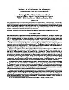
The containment labeling scheme is first suggested by Santoro and Khatib [32]. Yoshikawa and Amagasa [43] also proposed a variant of containment labeling scheme. To label the XML tree based on the containment scheme, different tree traversal methods (e.g. pre-and-postorder [15], extended preorder [26], multilevel recursive UID [22,23]) are used. Zhang et al [45] use a labeling scheme in which every node is assigned three values: “start”, “end” and “level”. For any two nodes u and v, u is an ancestor of v iff u.start < v.start and v.end < u.end. In other words, the interval of v is contained in the interval of u. Node u is a parent of node v iff u is an ancestor of v and v.level - u.level = 1. Node u is a sibling of node v iff the parent of node u is also a parent of node v. Node u is a preceding (following) node of node v iff u.start < (>) v.start. Figure 2 shows Zhang’s containment labeling scheme [45].

Wu et al [38] use Prime numbers to label XML trees. The root node is labeled with “1” (integer). Based on a top-down approach, each node is given a unique prime number (self label) and the label of each node is the product of its parent node’s label (parent label) and its own self label. For any two nodes u and v, u is an ancestor of v iff label(v) mod label(u) = 0. Node u is a parent of node v iff label(v)/self label(v) = label(u). Node u is a sibling of node v iff label(u)/self label(u) = label(v)/self label(v). Prime uses the SC (Simultaneous Congruence) values in Chinese Remainder Theorem [6, 38] to decide the document order, i.e. SC mod self label = document order, then it compares the document orders of two nodes.

1,18,1 4,9,2

2,3,2 5,6,3

10,11,2

12,17,2

13,14,3

7,8,3

15,16,3

Fig. 2 Containment scheme

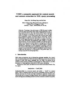
Prefix scheme. In prefix labeling schemes, the label of a node is the label of its parent’s label (prefix label) concatenated with its own label (self label). For any two nodes u and v, u is an ancestor of v iff label(u) is a prefix of label(v). Node u is a parent of node v iff label(v) has no prefix when removing label(u) from the left side of label(v). Node u is a sibling of node v if they have the same prefix label. Node u is a preceding (following) node of node v iff label(u) is smaller (larger) than label(v) lexicographically. DeweyID [35] labels the nth child of a node with an integer n, and this n should be concatenated to the prefix (its parent’s label) and delimiter (e.g. “.”) to form the complete label of this child node. Figure 3 shows DeweyID.

Example 2.1 Prime labels the root firstly, then the child of the root, and next the grandchild of the root. We consider one label in Figure 4. The 3rd (document order; the number above the node) node is labeled with “33” (the right number), which is the product of its parent label “3” and its self label “11”. Prime uses the SC (Simultaneous Congruence) value in Chinese Remainder Theorem [6,38] to decide the node order. Example 2.2 The SC value for the 8 nodes (except the root) in Figure 4 is 8965025. That is to say, 8965025 mod 2 = 1 (here 2 is the self label and 1 is the document order), 8965025 mod 3 = 2, . . . , 8965025 mod 17 = 7, and 8965025 mod 19 = 8. Prime only needs to store this SC value and the self labels rather than store the document order. 0 1

2

(1 ´

1

2

5 6 3 5 7 (1 ´ 7) 2) (1 ´ 3) (1 ´ 5) 7 8 3 4 119 133 33 39 (7 ´ 19) (3 ´ 11) (3 ´ 13) (7 ´ 17)

Fig. 4 Prime scheme

2.2 Encoding approaches Binary number encoding. 2

1 2.1

3 2.2

Fig. 3 DeweyID prefix scheme

4 4.1

4.2

In implementation, the containment labels are stored as binary numbers in a computer. Further, the binary numbers can be stored with either variable lengths or fixed lengths. Because the binary number encoding for integers is trivial, we do not discuss the details (see Section 4 for variable and fixed length binary number encodings).

4

Changqing Li et al.

Table 1 UTF8 encoding Value

Physical representation of self label

N < 128(27 ) 27 < N < 211 211 < N < 216 216 < N < 221 221 < N < 226

0xxxxxxx 110xxxxx 10xxxxxx 1110xxxx 10xxxxxx 10xxxxxx 11110xxx 10xxxxxx 10xxxxxx 10xxxxxx 111110xx 10xxxxxx 10xxxxxx 10xxxxxx 10xxxxxx 1111110x 10xxxxxx 10xxxxxx 10xxxxxx 10xxxxxx 10xxxxxx

226 < N < 231

UTF8 and OrdPath encodings to process delimiters. It should be noted that when implementing prefix labeling schemes, the delimiter “.” can not be stored together with the labels (numbers). To process the delimiters, different encodings are proposed. DeweyID uses UTF8 [41] encoding to process delimiters. In UTF8, a variable number of bytes are used to encode different integer values. If the integer value is smaller than 128 = 27 , it is encoded with one byte 0xxxxxxx where x represents the bits used for the integer value. If the integer value is between 27 and 211 , it is encoded with 2 bytes 110xxxxx 10xxxxxx. See Table 1 for more details. To represent an entire Dewey path with UTF8, each component of the path is encoded in UTF8 and then concatenated (without delimiter). The indicator bits “0”, “110”, “1110”, etc in the first byte (see Table 1) determine how many bytes are used and separate different components. Example 2.3 Consider a DeweyID label “1.129”. Since “1” is less than 128, “00000001” will be the UTF8 code of “1”. Since 129 is larger than 27 and less than 211 , the 11 bit binary encoding of 129 is “10000000001”, then the first five bits “10000” will be concatenated after “110”, and the rest six bits “000001” will be concatenated after “10” (see the third row of Table 1). The UTF8 code of 129 is “11010000 10000001”. Finally, the DeweyID “1.129” will be “000000011101000010000001”. Based on the indicators “0” and “110”, we know that the first component is stored with 1 byte, and the second component is stored with 2 bytes. In this way, DeweyID can separate different components without using the delimiter “.”. After processing the delimiter of DeweyID, we call it DeweyID(UTF8). OrdPath [30] has two kinds of encodings which are similar to UTF8 encoding. Compared with UTF8, the OrdPath [30] encodings are more compact. However, OrdPath needs more time to decode. Binary string and quaternary string encodings. Cohen et al [14] use Binary String to store the prefix labels, called BinaryString in this paper. The root of the

tree is labeled with an empty string. The first child of the root is labeled with “0”, the second child with “10”, the third with “110”, and the fourth with “1110” etc. Similarly for any node u, the first child of u is labeled with label(u).“0”, the second child of u is labeled with label(u).“10”, and the ith child with label(u).“1i−1 0”. The “0” in the labels can be used as the delimiter to separate different components of a label. The main part of this paper is about encodings. Our encodings are based on binary strings and quaternary strings. Compared with the binary string in [14], our binary string is compact and dynamic, and the quaternary string encoding in this paper is novel. The dynamic binary and quaternary string encodings in this paper can be applied broadly to different labeling schemes to efficiently process order-sensitive updates.

2.3 Existing approaches to process updates In this section, we discuss the approaches to process updates in labeling schemes. Float-point [5]. It should be noted that re-labeling in the containment scheme is not only to maintain the document order. If XML trees are not re-labeled after a node is inserted, the containment scheme can not work correctly to determine the ancestor-descendant, parent-child etc. relationships. To solve the re-labeling problem, [5] uses Float-point values for the “start” and “end” of intervals. It seems that Float-point solves the re-labeling problem [35]. But in practice, the Float-point is represented in a computer with a fixed number of bits [5,35]. As a result, at most 18 nodes [5] can be inserted at a fixed place since [5] uses the consecutive integer values at the initial labeling. Even if [5] uses values with large gaps, it still can not avoid re-labeling due to the float-point precision. Therefore, using real values instead of integers only provides limited benefits for the label updating [35,38]. OrdPath [30]. To keep the document order, the DeweyID(UTF8) and BinaryString prefix schemes need to re-label the sibling nodes after the inserted node and the descendants of these siblings. OrdPath [30] is a labeling scheme that can essentially process order-sensitive updates. OrdPath is similar to DeweyID, but it only uses odd numbers at the initial labeling (see Figure 5). When the XML tree is updated, it uses the even number between two odd numbers to concatenate another odd number. Example 2.4 Given three DeweyID labels “1”, “2” and “3”, we can easily know that they are siblings. In addition, given two DeweyID labels “2” and “2.1”, we can

Efficient updates in dynamic XML data: from binary string to quaternary string

3

1 3.1

5 3.3

7 7.1

7.3

Fig. 5 OrdPath prefix scheme

easily know that “2” is a parent of “2.1”. But for OrdPath (see Figure 5), its labels are “1”, “3”, “5” etc.; when inserting a label between “1” and “3”, it uses the even number between “1” and “3” i.e. “2” to concatenate another odd number i.e. “1” as the label of this inserted node, i.e. the inserted label is “2.1”. In OrdPath, “2.1” is at the same level as “1”, “3” etc., i.e. “2.1” is a sibling of “1” and “3”. Furthermore, when inserting one more node between “1” and “2.1”, OrdPath uses “2.-1” as the inserted label and “2.-1” is also the sibling of “1”, “2.1” and “3”. In this way, OrdPath need not re-label the existing nodes in insertions, however this makes OrdPath slow in determining the sibling, parent-child etc. relationships in XML query processing. Therefore OrdPath gets better update performance by reducing the query performance. This is not desirable. OrdPath can avoid the re-labeling to some extent, but it reduce the query performance and its update cost is expensive. (1) It wastes half of the total numbers compared to DeweyID (wastes the even numbers; even after insertion, it still wastes the even number, e.g. “2.0” between “2.-1” and “2.1” is still not used after insertion). (2) Though OrdPath1 and OrdPath2 encodings can reduce the label size compared to UTF8 encoding, it is slow for OrdPath1 and OrdPath2 to get back the number. This will influence both the query and update performance. (3) It can be seen from Example 2.3 that “1”, “2.-1”, “2.1” and “3” are at the same level, i.e. they are siblings. OrdPath needs more time to determine this based on the even and odd numbers (the even number is not a level) which will reduce its query performance. (4) OrdPath needs the addition and division operations to calculate the even number between two odd numbers which is expensive in updating. It is also possible that OrdPath only uses the addition operation to get the even number, but if there are many deletions, the insertion with only addition operation is a bias and the label size will increase fast. Moreover, even if OrdPath only uses the addition operation in processing updates, the addition operation is not so cheap. SC value in prime scheme. When the document order is changed, Prime only needs to re-calculate the SC values instead of re-labeling. Example 2.5 When a new sibling node is inserted before the 1st node (see Figure 4; the inserted node is now

5

the first child of the root), the next available prime number is 23, then the label of the new inserted node is 23 (1 × 23). This new inserted node becomes now the 1st node (document order), and the orders of the nodes after this inserted node should all be added with 1 (the old orders are calculated based on the old SC value). Prime calculates the new SC value for the new ordering, which is 28364406 such that 28364406 mod 23 = 1, 28364406 mod 2 = 2, 28364406 mod 3 = 3, . . . , 28364406 mod 17 = 8, and 28364406 mod 19 = 9. BOX [33]. The work in [42] is used for incremental maintenance of XML structural indexes [28] rather than maintenance of labels in labeling schemes. Silberstein et al [33] use Weight-Balanced B-Tree (W-BOX) and Back-Linked BTree (B-BOX) to provide a nice tradeoff between update and lookup costs for labeling schemes: W-BOX has logarithmic amortized update cost and constant worst-case lookup cost, while B-BOX has constant amortized update cost and logarithmic worst-case lookup cost. The objective of BOX [33] is to provide a good tradeoff between update and lookup costs. On the other hand, the objective of this paper and the work in Float-point [5], OrdPath [30] and Prime [38] are trying to avoid relabeling in XML updates. Comparisons. Although Prime supports order-sensitive updates without re-labeling the existing nodes, it needs to re-calculate the SC values based on the new ordering of nodes. The re-calculation is much more time consuming. The main idea of other labeling schemes [5,26] (except Prime) is to leave some unused values for future insertions. When the unused values are used up later, they have to re-label the existing nodes, i.e. they can not completely avoid re-labeling in XML leaf node updates. Though OrdPath [30] is dynamic to some extent to process the updates (will encounter the overflow problem; see Example 8.1), it needs to decode its codes and use the addition and division operations to calculate the even number between two odd numbers, which make its update cost not so cheap. In addition, the better update performance of OrdPath does not come without a cost. It wastes a lot of even numbers which makes its label size larger, and it needs more time to determine the prefix levels based on the even and odd numbers in XML query processing. The objective of BOX [33] is to provide a nice tradeoff between update and lookup cost rather than avoid relabeling. In this paper, we propose a novel Compact Dynamic Binary String (CDBS) encoding (CDBS is completely different from the encoding in [14]; the only common point is that they both use binary strings). The size of

6

Changqing Li et al.

our CDBS is as small as the binary number encoding of consecutive decimal numbers. As we know, there is no gap between two consecutive decimal numbers; that means our CDBS is the most compact and it need not leave unused values for future insertions. Yet our CDBS supports that CDBS codes can be inserted between any two consecutive CDBS codes. This is the most important benefit of our CDBS over the previous approaches. In addition, our CDBS can be applied broadly to different labeling schemes to process updates. Also our CDBS does not reduce the query performance. Moreover, to solve the overflow problem of CDBS, we improve CDBS to a Compact Dynamic Quaternary String (CDQS) encoding which can completely avoid re-labeling in XML leaf node updates. It seems that our CDBS is in the same family as OrdPath, but in fact independently; the idea of our CDBS comes from the division of numbers by 2. For example, given numbers 1 and 2, find the middle number between 1 and 2. CDQS which comes from the division by 4 is an extension of CDBS to solve the overflow problem. 3 Lexicographical order The most important feature of our approach is that we compare labels based on the lexicographical order rather than the numerical order. Definition 3.1 (Lexicographical order ≺) Given two binary strings SL and SR (SL represents the left binary string and SR represents the right binary string), SL is said to be lexicographically equal to SR iff they are exactly the same. SL is said to be lexicographically smaller than SR (SL ≺ SR ) iff (a) the lexicographical comparison of SL and SR is bit by bit from left to right. If the current bit of SL is 0 and the current bit of SR is 1, then SL ≺ SR and stop the comparison, or (b) SL is a prefix of SR . Next based on Algorithm 1, Theorem 3.1 and Example 3.2, we illustrate how to insert a binary string SM (SM represents the middle binary string) between two lexicographically ordered binary strings SL and SR such that SL ≺ SM ≺ SR lexicographically. Based on Algorithm 1, our CDBS encoding in Section 4 does not require re-labeling. Note that the last bit of SL and SR in Algorithm 1 is required to be 1. We use an example to show why we require the last bit of the binary string to be “1”. Example 3.1 Suppose there are two binary strings “0” and “00”. “0” ≺ “00” lexicographically because “0” is a prefix of “00”, but we can not insert a binary string SM between “0” and “00” such that “0” ≺ SM ≺ “00”. Accordingly we require the binary strings to be ended with “1”.

Algorithm 1: AssignMiddleBinaryString(SL , SR ) Input: SL ≺ SR ; SL and SR are both ended with “1” Output: SM (ended with 1) such that SL ≺ SM ≺ SR lexicographically 1 if size(SL ) ≥ size(SR ) then //Case (a) 2 SM = SL ⊕ “1”; //⊕ means concatenation 3 else if size(SL ) < size(SR ) then //Case (b) 4 SM = SR with the last bit “1” changed to “01”; 5 end 6 return SM ;

Theorem 3.1 Given any two binary strings SL and SR which are both ended with “1” and SL ≺ SR , we can always find a binary string SM based on Algorithm 1 such that SL ≺ SM ≺ SR lexicographically. Proof: Case (a): If size(SL ) ≥ size(SR ), we process SM based on lines 1 and 2 in Algorithm 1, i.e. SM = SL ⊕ “1”. (a1): SM is that SL concatenates one more “1”, thus SL is a prefix of SM . According to condition (b) in Definition 3.1, SL ≺ SM lexicographically. (a2): Since size(SL ) ≥ size(SR ) and SL ≺ SR , condition (a) in Definition 3.1 must be satisfied. That means there is a position; the bit of SL at this position is “0”, and the bit of SR at this position is “1”. Therefore when we concatenate one more “1” after SL i.e. SM , SM is still smaller than SR lexicographically (the lexicographical comparison is from left to right), i.e. SM ≺ SR . Based on (a1) and (a2), SL ≺ SM ≺ SR lexicographically when size(SL ) ≥ size(SR ). Case (b): If size(SL ) < size(SR ), we process SM based on lines 3 and 4 in Algorithm 1, i.e. SM = SR with the last bit “1” changed to “01”. (b1): If the first (size(SR )-1) bits of SR are larger than SL lexicographically, SL ≺ SM because SM is the first (size(SR )-1) bits of SR ⊕ “01”. If the first (size(SR )1) bits of SR are exactly the same as the SL , SL ≺ SM because SM is SL ⊕ “01” (SL is the same as the first (size(SR )-1) bits of SR ; SL is a prefix of SM ). Note that the first (size(SR )-1) bits of SR can not be smaller than SL lexicographically, otherwise SL will be larger than SR lexicographically (conflict to the condition in Theorem 3.1). Thus SL ≺ SM . (b2): If we do not consider the last two bits “01” of SM and the last bit “1” of SR , SM is exactly the same as SR , and “01” ≺ “1” lexicographically. Thus SM ≺ SR . Based on (b1) and (b2), SL ≺ SM ≺ SR lexicographically when size(SL ) < size(SR ). Therefore Theorem 3.1 holds. Example 3.2 To insert a binary string between “001” and “01”, the size of “001” is 3 which is larger than the size 2 of “01”, therefore we directly concatenate one more “1” after “001” (see lines 1 and 2 in Algorithm 1).

Efficient updates in dynamic XML data: from binary string to quaternary string

The inserted binary string is “0011” and “001” ≺ “0011” ≺ “01” lexicographically. To insert a binary string between “01” and “011”, the size of “01” is 2 which is smaller than the size 3 of “011”, therefore we change the last “1” of “011” to “01”, i.e. the inserted binary string is “0101” (see lines 3 and 4 in Algorithm 1); obviously “01” ≺ “0101” ≺ “011” lexicographically. Algorithm 1 is the foundation of this paper which can help to process updates efficiently. When the labeling scheme is a prefix scheme, based on Theorem 3.1, we can insert one label between two labels without re-labeling the existing nodes. When the labeling scheme is a containment scheme, we may need to insert the “start” and “end” two values at one place. The following Corollary 3.3 guarantees that two labels can be inserted between two labels without re-labeling. Lemma 3.2 The SM in Theorem 3.1 returned by Algorithm 1 is ended with “1”. Proof: This is obvious when we check Algorithm 1. Lines 1 and 2 indicate that the end bit of SM is “1” when size(SL ) ≥ size(SR ), and lines 3 and 4 indicate that the end bit of SM is “1” when size(SL ) < size(SR ), therefore SM is ended with “1”. Corollary 3.3 Given any two binary strings SL and SR which are both ended with “1” and SL ≺ SR , we can always find two binary strings SM 1 and SM 2 such that SL ≺ SM 1 ≺ SM 2 ≺ SR lexicographically. Proof: Based on Theorem 3.1, we can insert a binary string SM between SL and SR . Based on Lemma 3.2, we know that SM is also ended with “1”. Therefore based on Theorem 3.1, we can insert another binary string between SL and SM , or between SM and SR . Therefore Corollary 3.3 holds. We can further insert binary strings among SL , SM 1 , SM 2 and SR . Theorem 3.1 and Corollary 3.3 guarantee that we have low update cost in XML updating. Algorithm 1 proposed in this paper is dynamic and can be applied to any two ordered binary strings (ended with “1”) for insertions. On the other hand, to maintain the high query performance, we should not increase the label size when decreasing the update cost. In Section 4 we further propose a Compact Dynamic Binary String encoding, called CDBS. All the codes (binary strings) of CDBS are ended with “1” and CDBS encoding is as compact as the traditional binary number encoding (see Section 4). 4 A compact dynamic binary string encoding In this section, we propose a Compact Dynamic Binary String encoding (CDBS), and based on Algorithm 1, CDBS supports updates efficiently. We firstly use an example to illustrate how our CDBS encodes a set of numbers, and use examples to simply

7

Table 2 Binary and our CDBS encodings Decimal number

VBinary

VCDBS

FBinary

F-CDBS

1 2 3 4 5 6 7 8 9 10 11 12 13 14 15 16 17 18

1 10 11 100 101 110 111 1000 1001 1010 1011 1100 1101 1110 1111 10000 10001 10010

00001 0001 001 0011 01 01001 0101 011 0111 1 10001 1001 101 1011 11 1101 111 1111

00001 00010 00011 00100 00101 00110 00111 01000 01001 01010 01011 01100 01101 01110 01111 10000 10001 10010

00001 00010 00100 00110 01000 01001 01010 01100 01110 10000 10001 10010 10100 10110 11000 11010 11100 11110

Total size (bits)

64 (118 total)

64 (118 total)

90 (93 total)

90 (93 total)

analyze the total size of the CDBS codes. Next the formal encoding algorithm in Section 4.1 and the formal size analysis in Section 4.2 will be easier to understand. Table 2 shows the binary number encoding (V-Binary and F-Binary) and our CDBS (V-CDBS and F-CDBS) encoding of 18 numbers. We choose 18 as an example because the total “start” and “end” values in Figure 2 are 18. In fact, CDBS can encode any number (not only 18; see the formal algorithm in Section 4.1). When encoding 18 decimal numbers in binary, they are shown in Column 2 (V-Binary Column) of Table 2 which have Variable lengths, called V-Binary. Now let us discuss how to encode the 18 decimal numbers based on our CDBS encoding. Column 3 (VCDBS Column) of Table 2 shows our CDBS, which is called V-CDBS because it is also encoded with Variable lengths. The following steps show the details of how to get the V-CDBS codes (binary strings) and these steps are examples for the formal algorithm in Section 4.1. Step 1: In the encoding of the 18 numbers, we suppose there is one more number before number 1, say number 0, and one more number after number 18, say number 19. Step 2: We firstly encode the middle number with binary string “1”. The middle number is 10 where 10 is calculated in this way, 10 = round(0+(19-0)/2). The V-CDBS code of number 10 is “1” (see Table 2). Step 3: Next we encode the middle number between 0 and 10, and between 10 and 19. The middle number between 0 and 10 is 5 (5=round(0+(10-0)/2)) and the mid-

8

dle number between 10 and 19 is 15 (15=round(10+(1910)/2)). Step 4: To encode number 5, the code size of number 0 is 0 (the V-CDBS code of number 0 corresponding to SL in Algorithm 1 is empty now), and the code size of number 10 is 1 (the V-CDBS code of number 10 corresponding to SR in Algorithm 1 is “1” now with size 1 bit). This is Case (b) where size(SL ) < size(SR ) (see Algorithm 1). Thus based on lines 3 and 4 in Algorithm 1, the V-CDBS code of number 5 is “01” (“1” → “01”). Step 5: To encode number 15, the 10 th code (SL ) is “1” now with size 1 bit, and the 19 th code (SR ) is empty now with size 0. This is Case (a) where size(SL ) ≥ size(SR ) (see Algorithm 1). Therefore based on lines 1 and 2 in Algorithm 1, the V-CDBS code of number 15 is “11” (“1” ⊕ “1” → “11”). Step 6: Next we encode the middle numbers between 0 and 5, between 5 and 10, between 10 and 15, and between 15 and 19, which are numbers 3, 8, 13 and 17 respectively. The encodings of these numbers are still based on Case (a) or Case (b) in Algorithm 1. In this way, all the numbers except 0 will be encoded because the round function will reach the larger value (divided by 2), and we need to discard the V-CDBS code for number 19 since number 19 does not exist actually. With Step 1, we find that the total size of V-CDBS is equal to the total size of V-Binary (without Step 1, their total sizes are not always equal). Also the decimal numbers 1-18 can be encoded with Fixed length binary numbers, called F-Binary (F-Binary Column of Table 2). Since 18 needs 5 bits to store, zero or more “0”s should be concatenated before each code of V-Binary. On the other hand, when representing our CDBS using Fixed length, called F-CDBS, we concatenate “0”s after the V-CDBS codes (F-CDBS Column of Table 2). With Step 1 to Step 6 above, the formal encoding algorithm in Section 4.1 will be easier to understand, and with the following example illustration for the total code size, the formal size analysis in Section 4.2 will be easier to understand. Example 4.1 It can be seen from Table 2 that V-Binary has one code “1” with size 1 bit, two codes “10” and “11” with sizes 2 bits, four codes “100”, “101”, “110” and “111” with sizes 4 bits, etc., and the total size of V-Binary is 64 bits. Also we can see that our V-CDBS has one code “1” with size 1 bit, two codes “01” and “11” with sizes 2 bits, four codes “001”, “011”, “101” and “111” with sizes 4 bits, etc., and the total size of V-CDBS is also 64 bits. This means that our V-CDBS is as compact as the traditional binary number encoding. It is similar for F-Binary and F-CDBS (they both have size 90 bits).

Changqing Li et al.

Example 4.2 Table 2 shows that V-Binary has smaller total code size than F-Binary. However, we also need to store the size of each V-Binary code, the maximal size for a code is 5, e.g. the size of “10010” is 5 bits. We need to store this 5 using fixed length of bits (“101”; 3 bits). The sizes of other codes should also be stored using fixed length of bits (3 bits), therefore the total code size for V-Binary is 3×18+64=118 bits which is larger than the bits required by F-Binary. It is similar for V-CDBS and F-CDBS.

4.1 V-CDBS encoding algorithm Because F-CDBS is that some “0”s are concatenated after the V-CDBS codes, we focus on V-CDBS to introduce the algorithm. Algorithm 2 is the V-CDBS encoding algorithm. We use the procedure V-CDBS SubEncoding to get all the codes of the numbers. Finally number 0 and number (T N +1) should be discarded since they do not exist actually.

Algorithm 2: V-CDBS Encoding (T N ) Input: A positive integer T N Output: The V-CDBS codes for numbers 1 to T N 1 Suppose there is one more number before the first number, called number 0, and one more number after the last number, called number (T N + 1); 2 Define an array codeArr[0, T N + 1] //the size of //codeArr is TN+2; each element of the codeArr is //empty at the beginning; 3 V-CDBS SubEncoding(codeArr, 0, T N + 1); th 4 Discard the 0 and (T N +1)th elements of codeArr;

5 6 7 8 9 10

Procedure V-CDBS SubEncoding (codeArr, PL , PR ) /*V-CDBS SubEncoding is a recursive procedure; codeArr is an array, PL is the left position, and PR is the right position*/ PM = round((PL +PR )/2); if PL + 1 < PR then codeArr[PM ]=assignMiddleBinaryString(codeArr[PL ], codeArr[PR ]); V-CDBS SubEncoding(codeArr, PL , PM ); V-CDBS SubEncoding(codeArr, PM , PR ); end

V-CDBS SubEncoding is a recursive procedure, the input of which is an array codeArr, the left position “PL ” and the right position “PR ” in array codeArr. This procedure assigns codeArr[PM ] (corresponding to SM in Algorithm 1) using the AssignMiddleBinaryString algorithm (Algorithm 1), then it uses the new left and right positions to call the V-CDBS SubEncoding procedure itself, until each (except the 0 th ) element of the array codeArr has a value.

Efficient updates in dynamic XML data: from binary string to quaternary string

Note that SL and SR in the input of Algorithm 1 can be empty when it is called by V-CDBS SubEncoding here. If SL and SR are both empty, their sizes are both equal to 0, and SM is “1” based on lines 1 and 2 in Algorithm 1. If SL is empty and SR is not empty, size(SL ) < size(SR ), and we process SM based on lines 3 and 4 in Algorithm 1 (SM ≺ SR ). If SL is not empty and SR is empty, size(SL ) > size(SR ), and we process SM based on lines 1 and 2 in Algorithm 1 (SL ≺ SM ). Theorem 4.1 Given a positive integer TN, Algorithm 2 can encode all the numbers from 1 to TN with V-CDBS codes. Proof (Sketch): We simply illustrate why Theorem 4.1 holds. The V-CDBS encoding is like the binary search. As we know, the binary search will not miss any values in the search, therefore Algorithm 2 can encode each number without missing.

9

store this size, the bits required are log(log(N )), and the total bits required to store the sizes of all the variable codes are N log(log(N )). When taking formula (2) into account, the total sizes of V-Binary and V-CDBS are both N log(N + 1) + N log(log(N )) − N + log(N + 1) (3) F-Binary To store N numbers with fixed lengths, the size required is N log(N )

(4)

The size of the F-Binary code also needs to be stored, but needs to be stored only once with size log(log(N )). Therefore the total size for F-Binary is N log(N ) + log(log(N ))

(5)

Example 4.3 The V-CDBS codes in Table 2 are lexicographically ordered from top to bottom.

F-CDBS has the same total code size as formula (5).

The CDBS codes are ended with “1”, and lexicographically ordered, therefore we can insert without relabeling in updates based on CDBS.

Theorem 4.2 V-CDBS and F-CDBS are the most compact variable and fixed length dynamic binary string encodings. Proof (Sketch): As we know, the V-Binary and FBinary are encodings for the consecutive decimal numbers and there are no gaps between any two consecutive numbers, thus V-Binary and F-Binary are the most compact encodings. In addition, from the above size analysis, we know that our V-CDBS and F-CDBS have the same total sizes as V-Binary and F-Binary respectively2 . Therefore, our V-CDBS and F-CDBS are also the most compact.

4.2 Size analysis We analyze the size1 of different encodings. V-Binary For V-Binary, one number is stored with one bit (“1”; see Table 2), two numbers are stored with 2 bits (“10” and “11”), four numbers are stored with 3 bits (“100”, “101”, “110” and “111”), . . . , therefore the total size of V-Binary is 1 × 1 + 2 × 2 + 22 × 3 + 23 × 4 + . . . + 2n × (n + 1) = n × 2n+1 + 1

(1)

See Appendix for how to get formula (1).

5 Applying CDBS to different labeling schemes

Suppose the total number is N , which should be equal to 20 + 21 + 22 + . . . + 2n = 2n+1 − 1. Thus formula (1) becomes to N log(N + 1) − N + log(N + 1)

(2)

V-CDBS When considering our V-CDBS, it has one code (“1”) stored with one bit, two codes (“01” and “11”) stored with two bits, four codes (“001”, “011”, “101” and “111”) stored with three bits, . . . , therefore our V-CDBS has the same code size as V-Binary. In addition, since V-Binary and our V-CDBS have variable lengths, we need to store the size of each code. A fixed-length number of bits are used to store the size of the codes. The maximal size for a code is log(N ). To 1

Though the size of F-CDBS is smaller than the size of V-CDBS, it is easier for F-CDBS to encounter the overflow problem. See Section 8 for the overflow problem.

The size in this paper refers to bits, the log in this paper is used as the logarithm to base 2, and the log3 in this paper is used as the logarithm to base 3.

We firstly describe a property which is the second foundation of this paper (the first one is Theorem 3.1). Property 5.1 Our V-CDBS and F-CDBS are orthogonal to specific labeling schemes, thus they can be applied to different labeling schemes or other applications which need to maintain the order in updates. In this section, we mainly illustrate how our V-CDBS can be applied to different labeling schemes. F-CDBS is similar since it only concatenates zeros to V-CDBS codes. 2

We assume the consecutive numbers starting from 1. If the consecutive numbers start from 0, our approach can use “0” as one code in the encoding, then our approach still has the same size as Binary, but each time when we want to insert a code before “0”, we need to insert a code before the second code, and always put “0” as the first code.

10

Changqing Li et al.

When we replace the “start” and “end” values 1-18 of the containment scheme [45] (similar for other containment schemes [3,15,26,43]) in Figure 2 with the VCDBS codes in Table 2 and based on the lexicographical comparison, a V-CDBS based containment labeling scheme is formed, called V-CDBS-Containment. Similarly, we can replace the decimal numbers (see Figure 3) in the prefix labeling scheme with our V-CDBS codes, then a V-CDBS based prefix labeling scheme is formed, called V-CDBS-Prefix. We use the following example to show V-CDBS-Prefix. Example 5.1 From Figure 3, we can see that the root has 4 children. To encode 4 numbers based on Algorithm 2, the V-CDBS codes will be “001”, “01”, “1” and “11”. Similarly if there are two siblings, their self labels are “01” and “1”. Figure 6 shows V-CDBS-Prefix.

01

001 01.01

1 01.1

11 11.01

11.1

Fig. 6 V-CDBS-Prefix scheme (for Figure 3)

Similarly we can apply our V-CDBS to the prime labeling scheme to record the document order. But because Prime employs the modular and division operations to determine the ancestor-descendant etc. relationships, its query efficiency is quite bad (see Section 9 for the experimental results). Therefore we do not discuss in detail how V-CDBS is applied to Prime. It may be argued that V-CDBS only has the orders but does not have the exact position of each code, which seems a deficiency when compared to the V-Binary codes. For example, from a V-Binary code “110”, we can immediately know that “110” corresponds to the decimal number 6. However, if we delete the V-Binary codes “100” and “101”, “110” is now not the 6 th number but the 4 th number in order. In this paper, we focus on the dynamic XML data in which there are a lot of deletions and insertions, therefore V-Binary does NOT have merits over our V-CDBS in processing the nth position label. V-Binary and our V-CDBS both need to sort and get the position in the dynamic environment of XML. In addition, it is not to say that our V-CDBS can not immediately get the exact position. Based on an inverse processing of Algorithm 2, we can get the exact position of each V-CDBS code by calculations only. However, if the XML is static, we can directly use V-Binary rather than V-CDBS. If the XML is dynamic, none of them can calculate the positions immediately.

6 Processing of updates 6.1 Leaf node updates The deletion of nodes will not affect the relative orders of the nodes in XML. Hence we mainly discuss how to process the insertions based on V-CDBS. In this section, we use examples to show how to process the leaf node insertion based on our V-CDBS-Prefix and V-CDBS-Containment. Example 6.1 If we want to insert a sibling node before “01.01” in Figure 6, the self label of the inserted node is “001” (see lines 3 and 4 in Algorithm 1; the complete label is “01.001”). Theorem 3.1 guarantees that we need not re-label the existing nodes but we can keep the orders. The insertions at other places also need not re-label the existing nodes. Example 6.2 Similarly if we insert a sibling node before “5,6,3” in Figure 2, we should insert two values (“start” and “end”) between the start of “4,9,2” i.e. “4” and the start of “5,6,3” i.e. “5”. The existing schemes can not insert a number between “4” and “5”, but our V-CDBS codes for “4” and “5” are “0011” and “01” (see Table 2), and Corollary 3.3 guarantees that we can insert two binary strings between “0011” and “01” with the orders kept (the inserted two binary strings are “00111” and “001111”). That means we need not re-label the existing nodes, but we can keep the containment scheme working correctly. After insertion, we can further insert other nodes before the inserted node.

6.2 Internal node updates In [38], the internal node insertion problem has been studied, but all the existing labeling schemes have expensive internal node update cost. When inserting an internal node, the traditional containment scheme needs to re-label all the nodes after this inserted node in document order, all prefix schemes need to re-label the descendant nodes of the inserted node, and Prime also needs to re-label all the descendant nodes with the new inserted label multiplying all the labels of the descendants, in addition Prime needs to re-calculate the SC values. Furthermore, when deleting an internal node from the XML tree, all the containment, prefix and prime labeling scheme should re-label all the descendant nodes. That is to say, all the existing labeling schemes are not appropriate to process the internal node updates. When our V-CDBS are applied to the existing labeling schemes, V-CDBS-Containment can process the “start” and “end” values efficiently, but because the level values of all the descendants should be added with 1, the update cost is not so cheap. This is the drawback of the

Efficient updates in dynamic XML data: from binary string to quaternary string

existing containment schemes, but not the drawback of our CDBS encoding approach. To decrease the internal node update cost, we propose the P-Containment scheme. Rather than storing the “level” value in the containment scheme, P-Containment scheme stores the “parent start” value, which is the “start” value of the parent of this node. With the “parent start”, the parent-child relationship can be determined faster and the sibling relationship can be determined much faster. Note that to determine the sibling relationship, the traditional containment scheme should search the parent (need a lot of parent-child determinations) of a node, then determine whether another node is the child of this parent which is very expensive. The ancestor-descendant and ordering relationship determinations based on P-Containment are the same as the traditional containment labeling schemes. Figure 7 shows P-Containment. Example 6.3 In Figure 7, the “4” in “5,6,4” is the “parent-start” value, and it is equal to the “start” value of its parent, i.e. the “4” in “4,9,1”, therefore “4,9,1” is the parent of “5,6,4”. “5,6,4” is a sibling of “7,8,4” because their “parent start” values are both equal to “4”.

1,18,4,9,1

2,3,1 5,6,4

10,11,1

7,8,4

12,17,1

13,14,12

15,16,12

Fig. 7 P-Containment scheme

Theorem 6.1 P-Containment scheme requires that the “start” value of each node should be unique. Proof (Sketch): If the “start” of P-Containment is not unique, P-Containment may determine the parentchild etc. relationships wrongly. When V-CDBS is applied to P-Containment scheme, we call it V-CDBS-P-Containment. More important, the following Properties 6.1 and 6.2 show that our V-CDBSP-Containment has much cheaper internal node update cost. Property 6.1 Based on V-CDBS-P-Containment, when an internal node is inserted into the XML tree, the “parent start” of the inserted internal node should refer to the “start” of the parent of this internal node, the “parent start”s of the children of the inserted internal node should be modified to refer to the “start” of the inserted internal node, and the “parent start”s of all the descendants of the inserted internal node (except the children) need not be changed.

11

Example 6.4 When we replace the decimal numbers for the “start”, “end” and “parent start” values in Figure 7 with our V-CDBS codes (see Table 2 for the mappings), Figure 8 shows the V-CDBS-P-Containment scheme. Figure 8 also shows that an internal node “u” is inserted. We should insert a binary string between the “start” of the root and the “start” of the first child of the root, i.e. between “00001” and “0001”, as the “start” of node “u”. Based on Algorithm 1, the “start” of node “u” will be “000011”. Similarly the “end” of node “u” should be between “10001” and “1001” (see Figure 8; do not consider the insertion of the subtree now; Section 6.3 is about the insertion of a subtree) which will be “100011”. The “parent start” value of node “u” should be equal to the “start” value of the root, i.e. “00001”. The “parent start” of “0001,001,00001”, “0011,0111,00001” and “1,10001,00001” should be changed to refer to the “start” value of node “u”, i.e. change them to “000011”. The “start”, “end” and “parent start” values of the descendant nodes (of the children of node “u”) “01,01001,0011” and “0101,011,0011” need not be changed. Theorem 6.2 The “parent start” in P-Containment can not decrease the internal node insertion cost when the decimal numbers in the containment scheme are stored with V-Binary or F-Binary encodings. Proof: The “start” values of the descendants based on V-Binary and F-Binary need to be changed when inserting an internal node, therefore if we use the “start” of the parent as the “parent start” of the child, we still need to change the “parent start” values. The insertion cost will not be decreased. Only our V-CDBS-P-Containment (or F-CDBS-PContainment) is efficient to process the internal node insertion. The following property shows that our V-CDBS-PContainment has cheaper cost in processing the internal node deletions. Property 6.2 When an internal node is deleted from the XML tree, V-CDBS-P-Containment only needs to modify the “parent start” values of the child nodes of the deleted node to refer to the “start” value of the parent of the deleted node, but need not modify the “parent start” values of the descendant nodes of these child nodes. Our V-CDBS-P-Containment can greatly decrease the number of nodes to re-label in internal node updates. In addition, the “parent start” in P-Containment scheme can help to determine the parent-child relationship, especially the sibling relationship very fast. Moreover, the “parent start” is useful later in Section 8 to completely avoid re-labeling in leaf node updates. Prefix and prime schemes cannot be directly improved to process internal node updates efficiently as all the descendant labels themselves need to be modified.

12

Changqing Li et al. 00001,1111,00001

u 0001,001,00001

0011,0111,00001

01,01001,0011

1,10001,00001

subtree

1001,111,00001 101,1011,1001

0101,011,0011

11,1101,1001

Fig. 8 V-CDBS-P-Containment scheme, internal node insertion, and subtree insertion

6.3 Subtree updates The deletion of a subtree will not affect the relative orders of the rest nodes in the XML, hence we mainly discuss how to process the insertion of a subtree based on V-CDBS in this section. When a subtree is inserted into the XML tree, we can process the insertion of this subtree as the insertion of nodes one by one. However, this kind of insertion will make the label size increase fast (see Section 6.4 for more details). That is not what we expected. We use the following method to process the insertion of a subtree. Example 6.5 Figure 8 also shows that a subtree is inserted into the XML tree. For the subtree, we need to insert 8 binary strings (4 nodes; 8 “start” and “end” values) between the V-CDBS codes “10001” and “1001” in Figure 8. We use Algorithm 2 to process the insertion of the 8 binary strings, and “10001” and “1001” can be viewed as the V-CDBS codes for number 0 and number (TN+1)=(8+1)=9 in Algorithm 2. The middle number is the 5th number where 5 = round(0+(90)/2). The SL is “10001” with size 5 bits, and the SR is “1001” with size 4 bits, hence according to lines 1 and 2 in Algorithm 1 (called by Algorithm 2), the VCDBS code of the 5th number is “100011”. Similarly we can insert the V-CDBS codes for the rest 7 numbers. Finally the V-CDBS codes for these 8 numbers are “100010001”, “10001001”, “1000101”, “10001011”, “100011”, “10001101”, “1000111” and “10001111”. The inserted codes are ordered between “10001” and “1001” lexicographically. The “start” and “end” values of the four nodes of the subtree are “100010001, 10001111”, “10001001, 1000101”, “10001011, 100011”, and “10001101, 1000111”. We can get the “parent start” value of each node of the inserted subtree further. In this way, the label size will increase slower when inserting a subtree compared to the node by node insertions (see Section 9.3.3 for the experimental results). Similarly, we can use this method to process the insertion of a subtree based on the prefix scheme.

places. Therefore if a sequence of nodes are inserted random at different places of the XML tree, the size analysis in Section 4.2 is still valid, and the query performance will not be reduced. For the case that nodes are always inserted at a fixed place (we call it skewed insertion) of the XML tree, the size of our V-CDBS increases fast. [14] proves that any deterministic labeling scheme which does not re-label nodes must assign one label with size O(N ) in the worst case where N is the size of the XML tree. Our V-CDBS can not escape from this claim also, i.e. the label size of our V-CDBS increases linearly in the worst case. O(N ) is the upper bound of the size of our V-CDBS. OrdPath [30] also has this skewed insertion problem. [33] uses Btree to provide a tradeoff between update and lookup costs. The study in [11] shows that the insertions in XML data are often segments e.g. subtrees, and the insertion of single node seldom happens. As we can see from Section 6.3, the insertion of a subtree will not cause the label size increase fast. The above analysis also shows that our CDBS at least works very well when the insertions are random at different places of the XML tree. Even in the skewed insertion environment, our CDBS still works the best to answer queries (see the experimental results in Section 9.4). 7 Controlling the increase in label size In this section, we discuss how to control the increase in label size. If there are only insertions in updates, Algorithm 2 guarantees that the inserted code has the smallest size at that place, however if there are deletions as well, Algorithm 2 can not guarantee that the inserted code has the smallest size. Thus in Section 7.1, we design an algorithm which can find the code with the smallest size between two codes in the update environment with both insertions and deletions. Next in Section 7.2, we discuss some techniques to process the skewed insertion problem (see Section 6.4).

6.4 Uniformly and skewed insertions

7.1 Finding the codes with the smallest size between two codes (Reuse deleted codes)

The size analysis in Section 4.2 is based on the initial encoding. Algorithm 2 shows that our encoding algorithm is step by step insertions of nodes evenly at different

We firstly use an example to show why Algorithm 2 can not guarantee that the inserted binary string has the smallest size if there are deletions.

Efficient updates in dynamic XML data: from binary string to quaternary string

13

Algorithm 3: AssignMiddleBinaryStringWithSmallestSize(SL , SR ) Input: SL ≺ SR ; SL and SR are both ended with “1” Output: SM such that SL ≺ SM ≺ SR lexicographically, and SM has the smallest size 1 2 3 4 5 6 7 8 9 10 11 12 13 14 15 16 17 18 19 20 21 22 23 24 25 26 27

28 29 30 31 32 33 34 35 36 37 38

Case 1 SL is empty but SR is NOT empty, i.e. insert a code before the first code; denote the position of the firstly encountered “1” in SR as P ; //there must be a “1” in SR . ST = substring(SR , 1, P); //ST is the temporarily inserted binary string. if ST ≺ SR lexicographically then SM = ST ; //Case 1(a) else SM = substring(SR , 1, P-1) ⊕ “01”; //change the firstly encountered “1” to “01” //Case 1(b) end Case 2 SL is NOT empty but SR is empty, i.e. insert a code after the last code; if all the bits of SL are “1” then SM = SL ⊕ “1”; //Case 2(a) else //Case 2(b) denote the position of the firstly encountered “0” in SL as P ; SM = substring(SL , 1, P-1) ⊕ “1” //change the firstly encountered “0” to “1”; end Case 3 SL is a prefix of SR ; both SL and SR are not empty. Insert a code between two codes; ST = substring(SR , length(SL )+1, length(SR )); //ST is the temporarily inserted binary string when //removing SL from the left side of SR . denote the position of the firstly encountered “1” in ST as P //there must be a “1” in ST ; ST 2 = substring(ST , 1, P) //ST 2 is another temporarily inserted binary string; if ST 2 ≺ ST lexicographically then SM = SL ⊕ ST 2 ; //Case 3(a) else SM = SL ⊕ substring(ST , 1, P -1) ⊕ “01” //change the firstly encountered “1” to “01”; //Case 3(b) end Case 4 SL is not a prefix of SR ; both SL and SR are not empty. Insert a code between two codes; denote the first difference position of SL and SR as P ; ST = substring(SL , 1, P-1); //ST is the temporarily inserted binary before the first different //positions in SL and SR , i.e. SL = ST ⊕ ‘‘0" ⊕ ‘‘***", and SR = ST ⊕ ‘‘1" ⊕ ‘‘***". //Note that ‘‘***" is the rest binary string symbols. if length(SR ) > P then SM = ST ⊕ “1”; //Case 4(a) the P here is the P at line 26 else //i.e. length(SR ) = P ; note that length(SR ) can not be smaller than P ST 2 = substring(SL , P +1, length(SL )); //ST 2 is the temporarily inserted binary string from //position P +1 to the end position of SL . if all the bits of ST 2 are “1” then SM = SL ⊕ “0” ⊕ ST 2 ⊕ “1”; //Case 4(b) else //Case 4(c) denote the position of the firstly encountered “0” in ST 2 as P2 ; SM = ST ⊕ “0” ⊕ substring(ST 2 , 1, P 2-1) ⊕ “1” //change the firstly encountered “0” in ST 2 to “1”; end end

Example 7.1 For the first three V-CDBS codes “00001”, “0001” and “001” in Table 2, if we use Algorithm 1 to insert a binary string between “00001” and “0001”, the inserted binary string is “000011”. We can not find any other binary strings which are ended with “1”, are between “00001” and “0001” lexicographically, and have sizes smaller than or equal to 6 bits, i.e. the size of

“000011”. That is to say, if there are only insertions, Algorithm 1 guarantees that the inserted binary string always has the smallest size. On the other hand, if there are deletions also, Algorithm 1 can not guarantee that the inserted binary string has the smallest size. Suppose that we delete the “0001” between “00001” (SL ) and “001” (SR ). Now if we want to insert a binary

14

string between “00001” and “001”, the inserted binary is “000011” based on Algorithm 1. Obviously “000011” is not the binary string with the smallest size between “00001” and “001” because the size of the new code is 6 which is larger than the size of the deleted code “0001”. Therefore we design a new algorithm (Algorithm 3) to find the binary string with the smallest size between two binary strings in the update environment with both insertions and deletions. The main idea of Algorithm 3 is that we compare SL and SR bit by bit from left to right to find SM such that SM is ended with “1”, and SM has the smallest size in all the codes between SL and SR lexicographically. Now we use some intuitive examples to illustrate the different cases in Algorithm 3. (I) Case 1 in Algorithm 3 Case 1 is used to insert a code before the first code. The following intuitive example shows how Case 1 works. Example 7.2 Case 1(a), suppose we delete the first three V-CDBS codes in Table 2, and want to insert a binary string before the current first code “0011”. The firstly encountered “1” in “0011” is at the third position; thus ST = “001” (see Algorithm 3), and because ST ≺ SR , SM = ST = “001”. “001” is the binary string with the smallest size which is smaller than “0011” lexicographically. Case 1(b): suppose we delete the first VCDBS code in Table 2 and want to insert a binary string before the current first code “0001”. The firstly encountered “1” in “0001” is at the fourth position; thus ST = “0001”, but because ST is not lexicographically smaller than SR , i.e. the first code “0001”, we have to change the last “1” in ST to “01” as the final inserted binary string, i.e. the SM = “00001” (“0001” → “00001”). “00001” is the binary string with the smallest size which is smaller than “0001” lexicographically. (II) Case 2 in Algorithm 3 Case 2 is used to insert a code after the last code. The following intuitive example shows how Case 2 works. Example 7.3 Case 2(a), suppose we delete the last VCDBS code “1111” in Table 2 and want to insert a binary string after the current last code “111”. Because all the bits of “111” are “1”s, SM = SL ⊕ “1” = “1111” (see Algorithm 3). It can be seen that “1111” is the binary string with the smallest size which is large than “111” lexicographically. Case 2(b), suppose we delete the 13t h to 18th V-CDBS codes in Table 2, and want to insert a binary string after the current last code “1001”. We change the firstly encountered “0” to “1”. The firstly encountered “0” in “1001” is at the second bit; we change this “0” to “1”, and the inserted binary string is the first two bits of “1001” with “0” changed to “1”, i.e. SM = “11”. In this way, we guarantee that the inserted binary string is lexicographically larger than the last code and has the smallest size.

Changqing Li et al.

(III) Case 3 in Algorithm 3 Case 3 is used to insert a code between two codes. In Case 3, SL is a prefix of SR . The following intuitive example shows how Case 3 works. Example 7.4 Case 3(a), suppose we delete the two VCDBS codes between “11” (SL ) and “1111” (SR ) in Table 2, and want to insert a new binary string between SL “11” and SR “1111”. “11” ≺ “1111” lexicographically because “11” is a prefix of “1111”, therefore this is Case 3. ST = “11”, i.e. the last two bits of SR “1111” (see Algorithm 3). The firstly encountered “1” in ST is at the first position; thus ST 2 = “1” i.e. we assume that the temporarily inserted binary string is the first bit of “11”. ST 2 ≺ ST , thus SR = SL ⊕ ST 2 = “11” ⊕ “1” = “111”. Obviously “111” is the binary string with the smallest size between “11” and “1111” lexicographically. Similarly Case 3(b) can be processed following the steps for Case 3(b) in Algorithm 3; here we do not repeat these steps. (IV) Case 4 in Algorithm 3 Case 4 is still used to insert a code between two codes. In Case 4, SL is not a prefix of SR . The following intuitive example shows how Case 4 works. Example 7.5 Case 4(c), suppose we delete the second code between the first code “00001” (SL ) and the third code “001” (SR ) in Table 2, and want to insert a binary string between SL “00001” and SR “001”. “00001” ≺ “001” lexicographically because the third bit of “00001” is “0”, while the third bit of “001” is “1”, therefore this is Case 4. Because the first difference bit between “00001” and “001” is at position 3, ST = “00” (see Algorithm 3). Because length(SR ) = 3 which is not larger than the first difference position between SL and SR , ST 2 = “01”, i.e. the last two bits of SL “00001”. Because not all the bits of ST 2 are “1”s, this is Case 4(c). Finally SM = ST ⊕ “0” ⊕ subString(ST 2 , 1, P2-1) ⊕ “1” = “00” ⊕ “0” ⊕ “” ⊕ “1” = “0001”. Obviously SM “0001” is lexicographically between “00001” and “001” and it has the smallest size, i.e. there are no any other binary strings which are ended with “1”, are lexicographically between “00001” and “001”, and have smaller sizes as the inserted binary string “0001”. Similarly Case 4(a) and Case 4 (b) can be processed following the steps for Case 4(a) and Case 4(b) in Algorithm 3; here we do not repeat these steps. 7.2 Insertion skewness processing In Section 6.4, we discussed that the label size of our V-CDBS will increase fast if the nodes are always inserted at one fixed place. Here we further discuss some techniques to control the label size increasing speed in skewed insertion environment. Still based on V-CDBS, we introduce the skewness processing techniques.

Efficient updates in dynamic XML data: from binary string to quaternary string

Skewness Processing I (SPI) Estimate (based on the characteristics of the XML data or probing test) the number of nodes that will be inserted at the fixed place. Based on the estimated number, pre-calculate the labels, and assign these labels to the inserted nodes. Example 7.6 Suppose that there are 127 codes that are required to be inserted one by one before the first V-CDBS code “00001” (see Table 2), then each insertion requires that one more bit should be added for the new inserted code, i.e. the new code will be “000001”, “0000001”, “00000001” etc. Therefore the code size will increase fast; after inserting 127 codes, the total size for these 127 new codes will be (6+132)×127/2=8763. It can be seen that without any Skewness Processing Methods, the label size increases fast in the skewed insertion. On the other hand, if we employ the Skewness Processing Method (SPI), we can pre-calculate the codes for the 127 inserted codes at the beginning. Note that we pre-calculate the codes now, and assign the codes to the inserted nodes only when they are really inserted. The (1/2)th number of the 127 numbers is encoded with “000001” (“00001” → “000001”), the (1/4)th number of the 127 numbers is encoded with “0000001” (“000001” → “0000001”), and the (3/4)th number of the 127 numbers is encoded with “0000011” (“000001” ⊕ “1” → “0000011”). Similarly we can encode the (1/8)th , (3/8)th , (5/8)th and (7/8)th numbers of the 127 numbers. These steps are similar to the steps in Algorithm 2; the difference is that for this example, we know the most right code “00001”, but for Algorithm 2, both the most left and most right codes are empty at the beginning. In this way, the total size of the new inserted codes is 127×log(127+1) +4×127+log(127+1)=1404 for this example. It can be seen that 1404 is smaller than 8763, therefore SPI can efficiently process the skewed insertion problem. The method in Examples 7.6 can be used for the skewed insertions at other places, and not restricted to the insertions before the first code. Furthermore, if we know at the initialing labeling stage that nodes will always be inserted at a place, we can leave some codes with smaller sizes for this place. This can be known from the XML data manager about the feature of the XML data, e.g. the future stock data are always appended after the current stock data. Skewness Processing II (SPII) If we know that the nodes are always inserted at a fixed place, we can leave some codes with small sizes for this place at the initial labeling. Example 7.7 Suppose at the beginning, we know that the codes will always be inserted before the first code. Then at the beginning, we can suppose the first code is “1” (the most left code) and the most right code is empty, then we can encode all the numbers. Later when insertions happen, the size increases from 1 bit of “1” rather than from 5 bits of “00001” for the first V-CDBS code in

15

Table 2. It will be better if SPI and SPII can be combined together to process the skewness. SPI and SPII can be used for all the labeling schemes. It should be noted that the objective of this paper is to avoid re-labeling. Silberstein et al [33] use B-tree to balance the lookup and update costs. Obviously we can employ the method in [33] to process the skewed insertion problem. If re-labeling is allowed in the actual situation, our approach will not be worse than the existing approaches. If re-labeling is not allowed, only our approach support insertions without re-labeling (see Section 8 for more details). We use unbounded-length in our programming for XML data stored in files rather than in SQL DBMS. If our approach needs to be transferred to fit in SQL DBMS, we should improve the existing DBMS to support unbounded-length binary strings. Otherwise, we have to re-label if the length of a binary string exceeds 32 bits or 64 bits. From another view of point, this 32 bits or 64 bits may serve as a threshold for re-labeling in subtrees when employing the method in [33] to process skewed insertions. Again we need to emphasize that if the insertions are uniform, the label size of our approach increase logarithmically, it is the most compact, and it can be supported by the existing SQL DBMS.

8 CDQS encoding to completely avoid re-labeling in XML leaf node updates CDBS proposed in Section 4 still can not completely avoid re-labeling in XML leaf node updates. Here is an example. Example 8.1 The size of each V-CDBS code is stored with fixed length (e.g. 3; see Example 4.2). If many nodes are inserted into the XML tree, the size of the length field (e.g. 3) is not enough for the new labels, then we have to re-label all the existing nodes. Even if we increase the size of the length field (e.g. 3) to a larger number, it still can not completely avoid re-labeling, and it will waste the storage space. This is called the overflow problem in this paper. Similarly F-CDBS and OrdPath [30] will encounter the overflow problem also (O’Neil et al do not mention this overflow problem in OrdPath [30]). To solve the overflow problem, we have the following observation. We observed that the size of V-CDBS is used only to separate different V-CDBS codes. After separation, we can directly compare the V-CDBS codes from left to right. Therefore to solve the overflow problem, the way is to find a separator which can separate different V-CDBS codes; meanwhile this separator will not encounter the overflow problem. In binary string, there are only two symbols “0” and “1”; if we use “0” or “1” as the separator, only one symbol is left and CDBS will not be dynamic. Therefore we design a quaternary

16

Changqing Li et al.

Table 3 Our CDQS encoding Decimal number

CDQS

1 2 3 4 5 6 7 8 9 10 11 12 13 14 15 16 17 18

112 12 122 13 132 2 212 22 222 223 23 232 3 312 32 322 33 332

Total size (bits)

88 (124 total, including the separator size)

0 bit and the CDQS code of number 6 (SR ) is now “2” with size 2 bits. This is Case (b) where size(SL ) < size(SR ). In this case, the (1/3)th code is that we change the last symbol “2” of SR to “12”, i.e. the code of number 2 is “12” (“2” → “12”), and the (2/3)th code is that we change the last symbol “2” of SR to “13”, i.e. the code of number 4 is “13” (“2” → “13”). Note that in the initial encoding, if size(SL ) < size(SR ), SR can only be ended with “2” (can not be ended with “3”). Step 4: The (1/3)th and (2/3)th numbers between numbsers 6 and 13 are numbers 8 (8 = round(6+(13-6)/3)) and 11 (9 = round(6+(13-6)×2/3)). The CDQS code of number 6 (SL ) is “2” with size 2 bits and the code of number 13 (SR ) is “3” with size 2 bits. This is Case (a) where size(SL ) ≥ size(SR ). In this case, the (1/3)th code is that we directly concatenate one more “2” after the SL , i.e. the code of number 8 is “22” (“2” ⊕ “2” → “22”), and the (2/3)th code is that we directly concatenate one more “3” after the SL , i.e. the code of number 11 is “23” (“2” ⊕ “3” → “23”).

Step 2: The (1/3)th number is encoded with “2”, and the (2/3)th number is encoded with “3”. The (1/3)th number is number 6, which is calculated in this way, 6 = round(0+(19-0)/3). The (2/3)th number is number 13 (13 = round(0+(19-0)×2/3)).

Step 5: The (1/3)th and (2/3)th numbers between numbers 13 and 19 are numbers 15 (15 = round(13+(1913)/3)) and 17 (17 = round(13+(19-13)×2/3)). The code of number 13 (SL ) is “3” with size 2 bits and the code of number 19 (SR ) is empty now with size 0 bit. This is still Case (a) where size(SL ) ≥ size(SR ). Therefore the CDQS code of number 15 is “32” (“3” ⊕ “2” → “32”), and the code of number 17 is “33” (“3” ⊕ “3” → “33”). In this way, all the numbers will be encoded with our CDQS codes. Finally we need to discard the codes for numbers 0 and 19 since they do not exist actually. It should be noted that if the (2/3)th number exactly refers to the (1/3)th number, the code for the (2/3)th number will not appear since this number has already been encoded with the (1/3)th code. See Table 3 for the CDQS codes for all the 18 numbers. The formal algorithm of CDQS is similar to the VCDBS algorithm (Algorithms 1 and 2). The difference is that CDQS is based on the (1/3)th and (2/3)th positions rather than the (1/2)th position in V-CDBS. The above Step 1 to Step 5 are an illustration of the formal algorithms for CDQS. Here we do not repeat these two algorithms. Note that at the initial labeling stage, there are only two cases (Case (a) and Case (b)) to process. This is different from Algorithm 4 which is used for later insertions. It can be seen from Section 8.2 that Algorithm 4 needs to process more cases. When we note that the quaternary strings “0” ≺ “1” ≺ “2” ≺ “3” lexicographically, we have the following example.

Step 3: The (1/3)th and (2/3)th numbers between number 0 and number 6 are number 2 (2 = round(0+(60)/3)) and number 4 (4 = round(0+(6-0) 2/3)). The CDQS code of number 0 (SL ) is now empty with size

Example 8.2 The CDQS codes in Table 3 are lexicographically ordered from top to bottom, e.g. “112” ≺ “12” lexicographically since the second symbol of “112” is “1”, while the second symbol of “12” is “2”.

string encoding which can help to completely avoid relabeling in XML leaf node updates. 8.1 CDQS encoding Four symbols “0”, “1”, “2” and “3” are used in the quaternary string and each symbol is stored with two bits, i.e. “00”, “01”, “10” and “11”. Now we illustrate what is our Compact Dynamic Quaternary String (CDQS ) code, CDQS code is a special quaternary string; “0” is used as the separator and only “1”, “2” and “3” are used in the CDQS code itself. Because we use “0” as the separator, it is not appropriate to concatenate “0”s for the fixed length CDQS, i.e. F-CDQS. In this paper, when we talk about CDQS , it is equivalent to V-CDQS . Still based on the 18 numbers in Table 2, we use examples to show how CDQS works (see Table 3). Step 1: In the encoding of the 18 numbers based on CDQS, we suppose there is one more number before number 1, say number 0, and one more number after number 18, say number 19.

Efficient updates in dynamic XML data: from binary string to quaternary string

8.2 Processing of updates based on CDQS Algorithm 4 shows how to insert a quaternary string between two CDQS codes (two quaternary strings). Algorithm 4 considers the case that there are only insertions which is similar to Algorithm 1. If there are only insertions and size(SL ) < size(SR ), then SR can only be ended with “2”.

17

Though the total code size of CDQS is larger (10% around) than the total size of V-CDBS, and the update cost of CDQS is a little larger (modify 2 bits instead of 1 bit; consider more cases instead of two cases) than VCDBS, CDQS can completely avoid re-labeling in XML leaf node updates.

8.3 Reusing the deleted labels and applying CDQS to different labeling schemes Algorithm 4: AssignInsertedQuaternaryString(SL , SR ) Input: SL ≺ SR ; SL and SR are ended with “2” or “3” Output: SM such that SL ≺ SM ≺ SR lexicographically 1 if size(SL ) > size(SR ) then 2 if the last symbol of SL is “2” then 3 SM = SL with the last symbol changed from “2” to “3”; 4 else if the last symbol of SL is “3” then 5 SM = SL ⊕ “2”; //⊕ means concatenation 6 end 7 else if size(SL ) = size(SR ) then 8 SM = SL ⊕ “2”; 9 else if size(SL ) < size(SR ) then 10 SM = SR with the last symbol “2” changed to “12”; 11 end 12 return SM ;

Theorem 8.1 Algorithm 4 guarantees that a quaternary string can be inserted between two consecutive CDQS codes with the orders kept and without re-encoding any existing numbers. Proof (Sketch): When we check Algorithm 4, all the conditions can guarantee that SL ≺ SM ≺ SR lexicographically, therefore Theorem 8.1 holds. Corollary 8.2 Algorithm 4 guarantees that infinite number of quaternary strings can be inserted between any two consecutive CDQS codes. Proof (Sketch): When recursively using Algorithm 4 for the insertions, Corollary 8.2 holds. Theorem 8.3 CDQS can completely avoid re-labeling in XML leaf node updates. Proof: We use “0” as the separator to separate different CDQS codes, and “0” will never encounter the overflow problem. Also Corollary 8.2 guarantees that infinite number of quaternary strings can be inserted between any two consecutive CDQS codes. Therefore Theorem 8.3 holds. Section 6.2 shows that we can efficiently process the internal node updates though we can not completely avoid the re-labeling in internal node updates; this is the drawback the existing labeling schemes, but not the drawback of our CDQS encoding.

To reuse the deleted codes, similar to Algorithm 3, we can design an algorithm to reuse all the deleted CDQS codes. Here we do not repeat it. We can apply CDQS into different labeling schemes. For the containment scheme, since the “level” value will encounter the overflow problem, we only discuss how to apply CDQS to the P-Containment scheme (see Section 6.2 for the P-Containment scheme). When replacing the decimal numbers 1-18 of the “start”, “end” and “parent start” values of the P-Containment scheme in Figure 7 with our CDQS codes in Table 3, a CDQS based P-Containment scheme is formed. Based on the separator “0”, we can separate the “start”, “end” and “parent start” values, and each three values form a group of “start, end, parent start”. Example 8.3 For labels “1,18,-”, “2,3,1”, and “4,9,1” of the first three nodes of the P-Containment scheme in Figure 7, we store them consecutively in the hard disk as “112033201201220112013022201120” (see Table 3 for the mappings between the decimal numbers and the CDQS codes). Based on the separator “0”, we can separate them as “112”, “332”, “12”, “122”, “112”, “13”, “222” and “112”, the first two are a group of “start, end” which is the label of the root. It should be noted that the root does not have the “parent start” value. The next three are a group of “start, end, parent start” which is the label of the next node after the root. The rest three are another group of “start, end, parent start” which is the label of the third node. The labels for the 4th , 5th , etc. nodes can be similarly stored after the first three labels. We will never encounter the overflow problem, but we can separate different labels, and we can completely avoid re-labeling in XML leaf node updates. Note that in the implementation, each quaternary number is stored with two bits e.g. “2” is stored as “10” (two bits) in the implementation. Example 8.4 Figure 9 shows that we apply CDQS to the prefix scheme. The root has 4 children. To encode 4 numbers based on CDQS, the codes will be “12”, “2”, “3” and “32”. Similarly if there are two siblings, their self labels are “2” and “3”. See Figure 9 for CDQS-Prefix. For the prefix scheme, we use one separator “0” as the delimiter to separate different components of a label (e.g. separate “2” and “3” in “2.3”; the delimiter

18

Changqing Li et al.

9 Performance study 2

12 2.2

3 2.3

9.1 Experimental setup

32 32.2

32.3

Fig. 9 CDQS-Prefix scheme (for Figure 3)

“0” is equivalent to “.”; note “.” can not be stored together with numbers in the implementation), and use two consecutive “0”, i.e. “00”, as the separator to separate different labels (e.g. separate “2.2” and “2.3”). Example 8.5 To store the first three nodes “12”, “2” and “2.2” in Figure 9 (except the root which is empty) in the hard disk, they are stored as “120020020200”. Based on the separator “00”, we can separate “12”, “2” and “202”, and if necessary, we can separate different components of a label, e.g. separate “2” and “2” in “202” based on the delimiter “0”. It may be asked why we choose “0” but rather than any other quaternary number “1”, “2” or “3” as the delimiter? It is because in this way, we can directly compare two labels symbol by symbol from left to right to determine the document order. See the following example for more details. Example 8.6 Suppose that there is one more sibling node inserted between “2” and “3” in Figure 9. Based on Algorithm 4, the label of the inserted node is “22”. We know that “2.3” is before “22” (the label of the inserted node) in document order. “2.3” is stored as “203” with delimiter “0”. We can directly compare “203” and “22” from left to right to get the relative orders of these two labels. If we use any number of “1”, “2” or “3” as the delimiter, we cannot directly compare the labels from left to right to get the document order.

8.4 Extensions of CDBS and CDQS By further extending CDQS, we can use octal and hex string encodings to process updates, called CDOS and CDHS respectively. It can be seen from previous sections that CDQS grossly wastes 1/4 of the total numbers for the separator. If we use CDOS and CDHS encodings, only 1/8 and 1/16 of the total numbers are wasted grossly. Thus CDOS and CDHS encodings will be more compact when the total number is large. On the other hand, the separator sizes of CDOS and CDHS encodings are 3 bits and 4 bits respectively which will make CDOS and CDHS encodings not so compact as expected. See Section 9.2.4 for the experimental results.

We evaluate and compare the performance of different labeling schemes. The P-Containment scheme and the scheme names containing a “CDBS” or “CDQS” are all schemes proposed in this paper; all the others are prior schemes. The schemes with a “-Prefix” at the end of the scheme names are prefix schemes, and with a “Containment” at the end of the scheme names are containment schemes. All the schemes are implemented in Java and all the experiments are carried out on a 3.0 GHz Pentium 4 processor with 1 GB RAM running Windows XP Professional. Table 4 shows the characteristics of the test datasets. D1 is from [29], D3 and D4 are from [36], and all of them are real-world XML data. D2 is a benchmark generated by XMark [40]. We choose these datasets because they have different characteristics.

9.2 Performance study on static XML 9.2.1 Initial labeling In the implementation, we use SAX to parse the XML tree. Because we need to know the size of the tree, we need to scan the XML tree twice. At the first time, we label the XML tree based on the integers, then at the second time, we calculate the CDBS or CDQS codes based on the total number and replace the integers with our encodings. As we need to scan the XML tree twice, the initial labeling time based on our CDBS is larger than that of Binary labeling; the extra time is the initial labeling time of Binary labeling. However, this extra time is worthy because it makes the total label size of our CDBS as compact as the Binary encoding. Furthermore, Binary needs to re-label the existing nodes when inserting a node. Even one time re-labeling may need the extra initial labeling time. In addition, the initial labeling time is not so sensitive (do only once at the beginning; will not impact the query performance). Therefore, we say that this extra initial labeling time is worthy. After the initial labeling, we can freely insert labels without re-labeling and we need not know the total number of nodes later in the insertion. 9.2.2 Storage requirement In this section, we firstly test the label sizes of different (containment, prefix and prime) schemes, then we compare the label sizes of different containment schemes (include our containment schemes), and finally we compare the label sizes of different prefix schemes (include our prefix schemes). Figure 10(a) shows the label sizes of the existing containment, prefix and prime labeling schemes for the four datasets shown in Table 4. Prime [38] labeling scheme

Efficient updates in dynamic XML data: from binary string to quaternary string

19

Table 4 Test datasets Datasets

Topics

# of files

Max/average fan-out for a file

Max/average for a file

D1 D2 D3 D4

Shakespeare’s play XMark Treebank DBLP

37 1 1 1

434/48 25500/3242 56384/1623 328858/65930

6/5 12/6 36/8 6/3

has larger label size than the containment and prefix schemes because it skips a lot of integer numbers to get the prime numbers and it uses the multiplications of the numbers for the labels which both make its label size very large. Figure 10(b) is the comparison between the existing containment schemes and our CDBS and CDQS containment scheme. Float-point-Containment [5] has larger label size than other containment labeling schemes. VCDBS-Containment has the same label size as V-BinaryContainment, and F-CDBS-Containment has the same label size as F-Binary-Containment. These show that VCDBS and F-CDBS are the most compact variable and fixed length encodings. Because the separator “0” can not appear in the CDQS code itself which is a waste, the label sizes of CDQS-Containment are 10% around larger than the label sizes of V-CDBS-Containment for these datasets. Though the label size of CDQS-Containment is larger, CDQS-Containment can completely avoid relabeling in XML leaf node updates. When V-Binary, F-Binary, our V-CDBS, our F-CDBS and our CDQS are applied to the P-Containment scheme, V-CDBS-P-Containment still has the same label size as V-Binary-P-Containment, F-CDBS-P-Containment has the same size as F-Binary-P-Containment, and the label size of CDQS-P-Containment is still a little larger than the size of V-CDBS-P-Containment. Here we do not show the P-Containment schemes in Figure 10(b). For the prefix schemes, based on the size (length) of each code of our V-CDBS (similar for F-CDBS), we can use the UTF8 [41] or OrdPath [30] encoding to process the delimiters. If we use UTF8 to process the delimiters, our V-CDBS(UTF8)-Prefix has the same label size as DeweyID(UTF8)-Prefix. If we use OrdPath encodings to process the delimiters, our V-CDBS(OrdPath)-Prefix has smaller label size than OrdPath-Prefix since we do not waste the even numbers. As the UTF8 and OrdPath encodings are existing techniques, we do not compare the UTF8 or OrdPath encodings of our V-CDBS with DeweyID and OrdPath. In Section 8.3, we show how to process the delimiters based on our CDQS (see Example 8.5). Here in Figure 10(c), we compare the label size of our CDQS-Prefix with the existing prefix labeling schemes. It can be seen from Figure 10(c) that BinaryString-Prefix [14] has much larger label size than other prefix labeling schemes. Generally OrdPath1Prefix and OrdPath2-Prefix have smaller label sizes than

depth

Total # of nodes for each dataset 179689 1666315 2437666 3332130

Table 5 Test queries on the scaled D1 Queries

# of nodes retrieved

Q1:/play/act[4] Q2:/play//personae[./title]/pgroup[.//grpdescr] /persona Q3:/play/personae/persona[12]/preceding-sib ling::* Q4://act[2]/following::speaker Q5://act/scene/speech Q6:/play/*//line

370 2690 4240 184060 309330 1078330

DeweyID(UTF8)-Prefix though a lot of even numbers are wasted by OrdPath1-Prefix and OrdPath2-Prefix. This is because the encodings of OrdPath1 and OrdPath2 are more compact. However, though OrdPath decreases the label size, its query performance is worse on some queries because it needs more time to decode its encodings and needs more time to determine the levels based on the odd and even numbers (see Section 9.2.3). Our CDQS-Prefix has the smallest label sizes in all the four datasets (D1-D4) compared to the other prefix labeling schemes, and our CDQS-Prefix can completely avoid re-labeling in XML leaf node updates. Note that we use sizes to separate different DeweyID and OrdPath labels though different components of a DeweyID or OrdPath label can be separated by using UTF8 or OrdPath encodings. 9.2.3 Query performance Based on all the XML files in the Shakespeare’s play dataset (D1), we test the query performance, and for a more sizeable data workload we scaled up (replicated) D1 10 times as described in [35]. The ordered and un-ordered queries and the number of nodes retrieved are shown in Table 5. Different structural join algorithms [4,11,13,20,26, 37] have been proposed to process the XML queries. To do a fair comparison of different labeling schemes in the implementation, except the part which must be different, we use the same method (sort, join) to test the queries for all the labeling schemes. Figure 11 shows the response time (CPU time + I/O time) of the 6 queries in Table 5. Figure 11(a) shows the response time of the containment, prefix and prime labeling schemes. Prime has much larger response time because it has larger label size and it employs the modular and division operations

20

Changqing Li et al.

(a) Label sizes of different schemes

(b) Label schemes

sizes

of

containment

(c) Label sizes of prefix schemes

Fig. 10 Label sizes of different labeling schemes

(a) Response time of different schemes

(b) Response time of containment schemes

(c) Response time of prefix schemes

Fig. 11 Query performance of different labeling schemes

9.2.4 Performance Study on CDOS and CDHS When the total number is between 20 and 220 , Figure 12 shows the sizes of CDQS, CDOS, and CDHS. In Figure 12, we suppose that there is one separator for each code. When the total number is smaller than or equal to 28 , CDQS is the most compact; when the total number is between

25

LOG2(Total size (bits))

to determine the ancestor-descendant, parent-child etc. relationships which is very expensive. We compare containment scheme and prefix scheme fairly. Note that it is unfair if prefix labels are stored as strings, but containment labels are stored as integers. Figure 11(b) shows the response time of different containment schemes. Float-point has larger response time due to its very large label size. Our CDBS-Containment (“V-” and “F-”) has smaller response time than BinaryContainment (“V-” and “F-”) because our encodings can directly compare labels from left to right no matter the labels have variable or fixed lengths, but V-Binary can not directly compare labels from left to right. Finally Figure 11(c) shows the response time of different prefix schemes. BinaryString-Prefix has larger response time due to its larger label size on D1. Though OrdPath1-Prefix and OrdPath2-Prefix have smaller label sizes than DeweyID(UTF8)-Prefix, their query performance is worse than DeweyID(UTF8)-Prefix on some queries because it is slow for them to decode the OrdPath1 and OrdPath2 codes and slow to separate the prefix levels (OrdPath2 even slower). Our CDQS-Prefix has smaller response time on different queries because it has the smaller label size.

20 CDQS

15

CDOS 10

CDHS

5 0 0

2

4

6

8

10

12

14

16

18

20

LOG2(Total number)

Fig. 12 Label sizes of different labeling schemes

210 and 220 , CDOS is the most compact; and when the total number is larger than or equal to 216 , CDHS has smaller size than CDQS. Though with the increasing of the total number, the total size of CDOS and CDHS will be smaller than CDQS, the encoding time of CDOS and CDHS is averagely 2.1 and 5.5 times of that of CDQS. That is to say, CDOS and CDHS are slower in encoding. That also shows that CDOS and CDHS have more expensive update costs than CDQS. CDQS only needs to modify the last 2 bits of the neighbor codes, while CDOS and CDHS need to modify the last 3 and 4 bits respectively. More important, CDQS only needs to consider the neighbor code that is ended with “2” or “3” besides the sizes of the neighbor codes, while CDOS and CDHS need to consider many more cases to make the label size increase logarithmically, thus the update cost of CDOS and CDHS are not cheap; otherwise the sizes of CDOS and CDHS will increase very fast which makes

Efficient updates in dynamic XML data: from binary string to quaternary string Table 6 Number of nodes to re-label in leaf node updates Value

Number of nodes to re-label 1

2

3

4

5

Float-point-Containment V-Binary-Containment F-Binary-Containment V-CDBS-Containment F-CDBS-Containment CDQS-Containment

0 6596 6596 0 0 0

0 5121 5121 0 0 0

0 3932 3932 0 0 0

0 2431 2431 0 0 0

0 1300 1300 0 0 0

BinaryString-Prefix DeweyID(UTF8)-Prefix OrdPath1-Prefix OrdPath2-Prefix CDQS-Prefix

6595 6595 0 0 0

5120 5120 0 0 0

3931 3931 0 0 0

2430 2430 0 0 0

1299 1299 0 0 0

Prime

1320 1025 787

487

261

the advantage of CDOS and CDHS not an advantage, i.e. not more compact than CDQS. In conclusion, CDBS and CDQS are the cheapest two approaches to process updates, and their sizes are not large in practice. 9.3 Performance study on intermittent updates Section 9.3.1 discusses how to process the leaf node updates. Section 9.3.2 is about the internal node updates. Section 9.3.3 describes the performance when a subtree is inserted. 9.3.1 Leaf node updates The deletion of a leaf node will not require the re-labeling of existing nodes, therefore in this section we only compare the update performance when leaf nodes are inserted into the XML tree. Same as [38], we select one XML file Hamlet in D1 to test the update performance (it is similar for other XML files). Hamlet has 5 act elements. We test the following 5 cases (see Table 6 and Figure 13): inserting an act element before act[1], inserting an act element before act[2], . . . , and inserting an act element before act[5]. Table 6 shows the number of nodes to re-label when applying different labeling schemes. In the 5 cases, VBinary-Containment and F-Binary-Containment need to re-label many nodes (note that Hamlet has totally 6636 nodes). Though V-Binary-Containment and F-BinaryContainment are very compact, they need to re-label the existing nodes at each time when a node is inserted into the XML tree. BinaryString-Prefix and DeweyID(UTF8)-Prefix also need to re-label many nodes in the five insertion cases. It should be noted that V-Binary-Containment and FBinary-Containment have one more node to re-label than BinaryString-Prefix and DeweyID(UTF8)-Prefix because act elements are the children of the root and the containment schemes need to re-label the root also (modify the “end” value of the root).

21

For Prime, the number of SC values that are required to re-calculate is counted in Table 6. Because Prime uses each SC value for every five nodes [38], the number of SC values required to re-calculate is 1/5 of the number of nodes required by DeweyID(UTF8)-Prefix to re-label. Note that it is impossible to use a single SC value for all the nodes in the XML tree since the SC value will be a too large number. In the five cases, Float-point-Containment (less than 18 nodes at a single place), our V-CDBS-Containment (without overflow here), our F-CDBS-Containment (without overflow here), our CDQS-Containment (never need to re-label), OrdPath1-Prefix (without overflow here), OrdPath2-Prefix (without overflow here), and our CDQSPrefix (never need to re-label) need not re-label any existing nodes. Our V-CDBS-Containment and F-CDBSContainment are the most compact, yet they need not re-label the existing nodes in intermittent updates. Next we study the total time (CPU time + I/O time) for updates. Figure 13 shows the Log2 of the total leaf node update time (ms) (Y-axis). The total time required by Prime to re-calculate the SC values is much larger (at least 80 times; sum time of Case 1 to Case 5) than the time required by Binary-Containment (“V-” and “F-”) to re-label the nodes. Prime theoretically is a good scheme to process updates, but it is not practicable. The update time of BinaryString-Prefix [14] and DeweyID(UTF8) [35] is larger than the update time of Binary-Containment (“V-” and “F-”). In contrast, the total update time of V-CDBS-Containment, F-CDBSContainment, CDQS-Containment, and CDQS-Prefix is 1/12 to 1/3 of the time of Binary-Containment. This is because these approaches need not re-label the existing nodes.

Fig. 13 Log2 of total time (CPU time + I/O time) for leaf node updates

It can be seen from Figure 13 that the update performance differences among Float-point, OrdPath and our approach are not very large though our approach is still better. This is because only several nodes are inserted into the XML tree and the main part of the update time of Float-point, OrdPath and our approach is the I/O time. When considering the CPU time only, our approach is much better than Float-point and OrdPath.

22

Changqing Li et al.

Table 7 Number of nodes to re-label for internal node updates Number of nodes to re-label Insertion

Deletion

Float-point-Containment V-Binary-Containment F-Binary-Containment V-CDBS-Containment F-CDBS-Containment CDQS-Containment CDQS-P-Containment

6595 6596 6596 6595 6595 6595 5

6595 6595 6595 6595 6595 6595 5

BinaryString-Prefix DeweyID(UTF8)-Prefix OrdPath1-Prefix OrdPath2-Prefix CDQS-Prefix

6595 6595 6595 6595 6595

6595 6595 6595 6595 6595

Prime

6595

6595

Their wide update cost differences can be seen in Section 9.4 where frequent insertions are executed.

9.3.2 Internal node updates No matter an internal node is inserted into or deleted from an XML tree, the nodes should be re-labeled before the labeling schemes can work correctly to answer queries. Table 7 shows the number of nodes to re-label when inserting a node acts as the parent of the five act nodes in Hamlet and when deleting this internal node acts. It can be seen that all the labeling schemes except our CDQS-P-Containment (V-CDBS and F-CDBS can be applied to P-Containment scheme also; here we do not show them because they will encounter the overflow problem) need to re-label many nodes in internal node updates. Though our CDQS-P-Containment also needs to re-label the child nodes of the inserted node, it need not re-label the other descendant nodes of the inserted node, therefore it only needs to re-label 5 nodes which is much better than the existing approaches. Figure 14 shows the Log2 of the total internal node update time (ms) (Y-axis). For V-Binary-Containment and F-Binary-Containment, the deletion of an internal node needs less update time than the insertion of an internal node, because the deletion only needs to modify the “level” values, but the insertion needs to modify the “start”, “end” and “level” values. CDBS-Containment (“V-” and “F-”) only need to modify the “level” values, but need not modify the “start” and “end” values even in insertions, therefore their insertion time is smaller. The update time of Float-pointContainment is larger because its label size is larger which needs more I/O time. In contrast, our CDQSP-Containment needs much less update time because it needs to re-label much less nodes (5 vs 6595 or 6596).

Fig. 14 Log2 of total time (CPU time + I/O time) for internal node updates

All the prefix labeling schemes including our CDQSPrefix need to re-label all the descendant nodes when an internal node is inserted or deleted. When an internal node is updated, Prime needs to re-label all the descendant nodes of the inserted node. When an internal node is inserted, all the labels of the descendant nodes should multiply the label of the inserted node. When an internal node is deleted, all the labels of the descendant nodes should divide the label of the deleted node. In addition, Prime needs to recalculate the SC values to maintain the document order in insertions. Therefore the insertion time of Prime is much larger which can be seen from Figure 14. 9.3.3 Subtree insertion In this section, we discuss how to insert a subtree. If we insert the nodes of the subtree one by one, the label size will increase fast. If we insert the nodes of the subtree based on the method introduced in Section 6.3, the label size increases slowly. Figure 15 shows the label size increasing speed of these two methods when inserting subtrees with different number of nodes. It can be seen from Figure 15 that the label size based on the method introduced in Section 6.3 increases much slower than the method of insertions of subtrees node by node.

0.8

Label sizes (1,000,000 bits)

Value

0.7

Sequential insertion

0.6

Whole subtree insertion

0.5 0.4 0.3 0.2 0.1 0 0

200

400

600

800

1000

1200

Number of nodes in the inserted subtree

Fig. 15 Label size increasing when inserting a subtree

9.4 Performance study on frequent updates In the previous section, we study the performance when nodes are intermittently inserted into XML data.

20 18 16 OrderPath1-Prefix

14

OrderPath2-Prefix

12

CDQS-Prefix

10 8 6 0

150000

300000

LOG2(total update time (ms))

LOG2(total update time (ms))

Efficient updates in dynamic XML data: from binary string to quaternary string

23

24 22 20 18 16

Float-pointContainment

14

CDQS-Containment

12 10 8 6

450000

0

Number of nodes inserted

150000

300000

450000

Number of nodes inserted

(a) OrdPath-Prefix (1&2) vs CDQS-Prefix

(b) Float-point-Containment vs CDQS-Containment

14 13 12 11 10 9 8 7 6 5 4 3

OrdPath1-Prefix OrdPath2-Prefix CDQS-Prefix

0

50

100

150

200

Number of nodes inserted

(a) OrdPath-Prefix (1&2) vs CDQS-Prefix

LOG2(total update time (ms))

LOG2(total update time (ms))

Fig. 16 Uniformly frequent updates 20 18 16 14

Float-pointContainment

12

CDQSContainment

10 8 6 4 2 0

50

100

150

200

Number of nodes inserted

(b) Float-point-Containment vs CDQS-Containment

Fig. 17 Skewed frequent updates

In intermittent insertions, V-Binary-Containment, FBinary-Containment, BinaryString-Prefix, DeweyID(UTF8)-Prefix, and Prime have much larger update time; it will be even worse for them to update the XML tree with frequent and tiny insertions; this makes them impossible to answer queries in either the uniformly frequent or skewed frequent insertion environment. In this section, we mainly compare the update performance between OrdPath-Prefix (OrdPath1-Prefix and OrdPath2Prefix) and our CDQS-Prefix, and between Float-pointContainment and our CDQS-Containment. We compare our CDQS with the existing labeling schemes because frequent updates is easy to lead to overflow, and our CDQS can completely avoid re-labeling in XML leaf node updates. Section 9.4.1 discusses the case that frequent insertions are random at different places of the XML tree. Section 9.4.2 discusses the worst case that frequent and tiny insertions are always at a fixed place of the XML tree. 9.4.1 Uniformly frequent updates In this section, we test the uniformly distributed frequent insertions. The Hamlet file has totally 6636 nodes. We insert 6635 nodes between every two consecutive nodes of the 6636 nodes. Based on the new file after insertion, we insert another 13270 nodes between any two consecutive nodes. We repeat this kind of insertion 6 times. After the 6 th time insertion, the node number in the XML tree is 424641 which is 63.99 times of the original node number. Figures 16(a) and 16(b) show the Log2 of the total update time (ms) (Y-axis) of prefix schemes (OrdPath-

Prefix [30] vs CDQS-Prefix) and containment schemes (Float-point-Containment [2] vs CDQS-Containment) respectively. In frequent updates, the main part of the total update time is the CPU time since we can read the file at one time and write back all the updates at different places to the hard disk at one time. Even in frequent writing back, our approach still can save a lot of update time because the label size of CDQS-Prefix is smaller than the label size of OrdPath-Prefix and the label size of CDQS-Containment is smaller than the label size of Float-point-Containment. Even if overflow is not encountered, i.e. without relabeling, the update time of OrdPath-Prefix is still at least 207 (218.8−11.1 = 27.7 ) times of that of CDQS-Prefix (see Figure 16(a)). OrdPath needs to decode its codes [30] and needs the addition and division operations to get the numbers between two numbers which are both expensive. CDQS-Prefix only needs to modify the last 2 bits of the neighbor label to get the inserted label which is cheaper. Even if overflow is not encountered (less than 18 nodes at a fixed place), i.e. without re-labeling, the update time of Float-point-Containment (need to insert two values “start” and “end”; the calculation is expensive) is still at least 548 (29.1 ) times of that of CDQSContainment (see Figure 16(b)). When there is overflow, the update time of OrdPathPrefix and Float-point-Containment is even larger. If we can increase the length field of V-CDBS code a little larger, the uniformly frequent updates will not be so easy to lead V-CDBS to re-labeling. In addition, be-

24

Changqing Li et al.

9.4.2 Skewed frequent updates In this section, we test the case that the nodes are always inserted at a fixed place of the XML file Hamlet. When nodes are always inserted at a fixed place, OrdPath-Prefix and Float-point-Containment is much easier to encounter the overflow problem. Figure 17 shows that the update time of OrdPath-Prefix and Float-pointContainment is more than 1000 times larger than that of CDQS-Prefix and CDQS-Containment in skewed insertions. Thus CDQS is much better than OrdPath and Float-point in processing skewed frequent updates.

9.5.2 Processing the skewed insertion Figure 19 shows that the skewness processing techniques SPI and SPII introduced in Section 7.2 can efficiently to process the skewed insertion problem.

28

LOG2(Total label size (bits))

cause V-CDBS only needs to modify the last 1 bit of the neighbor label to get the inserted label, its update cost is smaller than the update cost of CDQS which needs to modify the last 2 bits of the neighbor label. Therefore V-CDBS can process the uniformly frequent updates more efficiently compared to CDQS if there is no overflow. Note that the update costs of OrdPath-Prefix and Float-point-Containment are much more expensive than V-CDBS and CDQS even if there is no overflow.

26 24 NoSP

22

SPI SPI+SPII

20 18 16 0

2500

5000

7500

Number of inserted nodes

Fig. 19 Processing of skewed insertions

10 Conclusion and future work 10.1 Summary of contributions

9.5 Controlling the increase in label size

Fig. 18 Comparison of Algorithm 1 and Algorithm 3 with deletions

10.1.1 Update We propose a novel Compact Dynamic Binary String (CDBS) encoding which is orthogonal to specific labeling schemes, therefore it can be applied broadly to different labeling shemes, e.g. containment, prefix and prime schemes, to maintain the document order when XML is updated. In addition, we improve our CDBS to a Compact Dynamic Quaternary String (CDQS) encoding which is also orthogonal to specific labeling schemes and can be applied to different labeling schemes. Though the total size of CDQS is larger (10% around) than the total size of CDBS, and though the update cost of CDQS is larger (modify the last 2 bits of the neighbor code instead of the last 1 bit; determine the neighbor code is ended with ”2” or ”3”) than CDBS, CDQS can completely avoid relabeling in XML leaf node updates. Furthermore, to efficiently process the internal node updates, we propose the P-Containment scheme which stores the “parent start” instead of the “level”. In this way, we can process the internal node updates much more efficiently based on our CDBS or CDQS encoding. The traditional encodings can not process the internal node update efficiently even if they employ the P-Containment scheme (see Theorem 6.2). Our V-CDBS and CDQS only need to modify the last 1 and 2 bits of the neighbour label to get the label of the inserted node which is the cheapest compared to the existing techniques. The experimental results show that our CDQS is the only approach to process frequent insertions efficiently.

The experimental results confirm that Algorithm 3 can reuse all the deleted labels, thus it efficiently controls the increase of the label size.

10.1.2 Query When XML is frequently updated, all the time for all the existing labeling schemes are used for the updates, thus they have no time to answer queries.

9.5.1 Reusing the deleted labels We test the case that nodes are deleted and inserted at the odd positions of Hamlet; after the deletions and insertions, we call this new Hamlet file Hamlet2 ; this is case 1. Secondly we test that the nodes are deleted and inserted at the even positions of Hamlet2, thirdly odd positions of Hamlet3, fourthly even positions of Hamlet4, and so on. We compare the performance of Algorithm 1 (original) and Algorithm 3 (Reuse). Figure 18 shows that the label size of Algorithm 3 does not increase in all the ten cases (since we reuse all the deleted labels). On the other hand, the label size of Algorithm 1 increases linearly (for these ten cases) which is fast. Note if there are only insertions (no deletions) at different places of the XML tree, the label size of Algorithm 1 increases logarithmically but not linearly.

Label size (1,000,000 bits)

0.4 Original algorithm (Algorithm 1)

0.3 0.2

Reuse Algorithm (Algorithm 3)

0.1 0 1

2

3

4

5

6

7

8

9

10

Deletion and insertion cases

Efficient updates in dynamic XML data: from binary string to quaternary string

Our approaches have better query performance than the existing labeling schemes in the environment of updates because we avoid the re-labeling and the update time of our approaches is much smaller. When considering the static environment of XML, for the containment scheme, our CDBS almost has the same total label size as Binary. Our CDQS increases the label size of V-CDBS a little. For the prefix scheme, our CDQS-Prefix have smaller label sizes than the existing prefix labeling schemes. The query performance of our approaches is not worse even in the static environment of XML.

10.2 Future work There are no labeling schemes or encoding approaches which can completely avoid re-labeling in internal node updates. Thus we need to consider how to solve this problem in the future. It can be seen from this paper that even if we do not handle the skewed insertion problem, our approaches still work the best to answer queries in the frequent update environment of XML because the update time of our approaches is much smaller. Also we propose techniques to process the skewed insertion problem, but these skewness processing techniques have some restrictions, e.g. they should estimate the number of nodes to be inserted at a fixed place, while the estimation will not be so easy. By balancing the query and update performance [33] or by re-labeling some nodes, we can solve this skewed insertion problem better. In the future, we want to research whether there are approaches that can completely avoid re-labeling and meanwhile solve the skewed insertion problem efficiently, but seems that it is not so easy to solve this problem because seems that these two aspects contradict each other.

References 1. S. Abiteboul, H. Kaplan, and T. Milo. Compact labeling schemes for ancestor queries. In Proc. of the 12th annual ACM-SIAM Symp. on Discrete Algorithms (SODA’01), pages 547-556, 2001. 2. S. Abiteboul and V. Vianu. Regular path queries with constraints. In Proc. of the 16th ACM Symp. on Principles of Database Systems (PODS’97), pages 122-133, 1997. 3. R. Agrawal, A. Borgida, and H.V. Jagadish. Efficient Management of Transitive Relationships in Large Data and Knowledge Bases. In Proc. of the ACM SIGMOD Int. Conf. on Management of Data (SIGMOD’89), pages 253262, 1989. 4. S. Al-Khalifa, H.V. Jagadish, J.M. Patel, Y. Wu, N. Koudas, and D. Srivastava. Structural Joins: A Primitive for Efficient XML Query Pattern Matching. In Proc. of the 18th Int. Conf. on Data Engineering (ICDE’02), pages 141-152, 2002.

25

5. T. Amagasa, M. Yoshikawa, and S. Uemura. QRS: A Robust Numbering Scheme for XML Documents. In Proc. of the 19th Int. Conf. on Data Engineering (ICDE’03), pages 705-707, 2003. 6. J.A. Anderson and J.M. Bell. Number Theory with Application. Prentice-Hall, New Jersey, 1997. 7. A. Berglund, S. Boag, D. Chamberlin, M.F. Fernandez, M. Kay, J. Robie, and J. Simon. XML path language (XPath) 2.0. W3C working draft 04, Apr. 2005. 8. S. Boag, D. Chamberlin, M.F. Fernandez, D. Florescu, J. Robie, and J. Simon. XQuery 1.0: An XML Query Language. W3C working draft 04, Apr. 2005. 9. T. Bray, J. Paoli, C.M. Sperberg-McQueen, E. Maler, F. Yergeau, and J. Cowan. Extensible markup language (XML) 1.1. W3C recommendation, Feb. 2004. 10. N. Bruno, N. Koudas, and D. Srivastava. Holistic twig joins: Optimal XML pattern matching. In Proc. of the ACM SIGMOD Int. Conf. on Management of Data (SIGMOD’02), pages 310-321, 2002. 11. B. Catania, W.Q. Wang, B.C. Ooi, and X. Wang. Lazy XML Updates: Laziness as a Virtue of Update and Structural Join Efficiency. In Proc. of the ACM SIGMOD Int. Conf. on Management of Data (SIGMOD’05), 2005. 12. T. Chen, J. Lu, and T.W. Ling. On Boosting Holism in XML Twig Pattern Matching using Structural Indexing Techniques. In Proc. of the ACM SIGMOD Int. Conf. on Management of Data (SIGMOD’05), 2005. 13. S.-Y. Chien, Z. Vagena, D. Zhang, V.J. Tsotras, and C. Zaniolo. Efficient Structural Joins on Indexed XML Documents. In Proc. of the 28th Int. Conf. on Very Large Data Bases (VLDB’02), pages 263-274, 2002. 14. E. Cohen, H. Kaplan, and T. Milo. Labeling Dynamic XML Trees. In Proc. of the 21st ACM Symp. on Principles of Database Systems (PODS’02), pages 271-281, 2002. 15. P.F. Dietz. Maintaining order in a linked list. In Proc. of the 14th Annual ACM Symp. on Theory of Computing (STOC’82), pages 122-127, 1982. 16. M. Fernandez and D. Suciu. Optimizing Regular Path Expres-sions Using Graph Schemas. In Proc. of the 14th Int. Conf. on Data Engineering (ICDE’98), pages 14-23, 1998. 17. G. Gottlob, C. Koch, and R. Pichler. XPath Query Evaluation: Improving Time and Space Efficiency. In Proc. of the 19th Int. Conf. on Data Engineering (ICDE’03), pages 379-390, 2003. 18. A. Halverson, J. Burger, L. Galanis, A. Kini, R. Krishnamurthy, A. N. Rao, F. Tian, S. Viglas, Y. Wang, J. F. Naughton, and D. J. DeWitt. Mixed mode XML query processing. In Proc. of the 29th Int. Conf. on Very Large Data Bases (VLDB’03), pages 225-236, Berlin, Germany, September 2003. 19. H. V. Jagadish, S. Al-Khalifa, A. Chapman, L. V. S. Lakshmanan, A. Nierman, S. Paparizos, J. M. Patel, D. Srivastava, N. Wiwatwattana, Y. Wu, and C. Yu. TIMBER: A native XML database. The VLDB Journal, 11(4):274-291, 2002. 20. H. Jiang, H. Lu, W. Wang, and B.C. Ooi. XR-Tree: Indexing XML Data for Efficient Structural Joins. In Proc. of the ACM SIGMOD Int. Conf. on Management of Data (SIGMOD’03), pages 253-263, 2003. 21. E. Jiao, T.W. Ling, and C.Y. Chan. PathStack : A Holistic Path Join Algorithm for Path Query with not-predicates

26 on XML Data. In Proc. of the 10th Int. Conf. on Database Systems for Advanced Applications (DASFAA’05), pages 113-124, 2005. 22. D.D. Kha, M. Yoshikawa, and S. Uemura. A Structural Number-ing Data. In Proc. of the 8th Int. Conf. on Extending Database Technology (EDBT’02) Workshop, pages 91-108, 2002. 23. D.D. Kha, M. Yoshikawa, and S. Uemura. An XML Indexing Structure with Relative Region Coordinate. In Proc. of the 17th Int. Conf. on Data Engineering (ICDE’01), pages 313-320, 2001. 24. Chanqing Li and Tok Wang Ling. QED: A Novel Quaternary En-coding to Completely Avoid Re-labeling in XML Updates. In Proc. of the 14th Int. Conf. on Information and Knowledge Man-agement (CIKM’05), pages 501-508, 2005. 25. Changqing Li, Tok Wang Ling, and Min Hu. Efficient Processing of Updates in Dynamic XML data. In Proc. of the 22nd Int. Conf. on Data Engineering (ICDE’06), 2006. 26. Q. Li and B. Moon. Indexing and Querying XML Data for Regu-lar Path Expressions. In Proc. of the 27th Int. Conf. on Very Large Data Bases (VLDB’01), pages 361370, 2001. 27. J. Lu, T. Chen, T.W. Ling. Efficient processing of XML twig pat-terns with parent child edges: a look-ahead approach. In Proc. of the 13th Int. Conf. on Information and Knowledge Management (CIKM’04), pages 533-542, 2004. 28. T. Milo and D. Suciu. Index Structures for Path Expressions. In Proc. of the 7th Int. Conf. on Database Theory (ICDT’99), pages 277-295, 1999. 29. NIAGARA Experimental Data. Available at: http://www.cs.wisc.edu/niagara/data.html 30. P.E. O’Neil, E.J. O’Neil, S. Pal, I. Cseri, G. Schaller, and N. Westbury. ORDPATHs: Insert-Friendly XML Node Labels. In Proc. of the ACM SIGMOD Int. Conf. on Management of Data (SIGMOD’04), pages 903-908, 2004. 31. P. Rao and B. Moon. PRIX: Indexing And Querying XML Using Pr¨ ufer Sequences. In Proc. of the 20th Int. Conf. on Data Engi-neering (ICDE’04), pages 288-300, 2004. 32. N. Santoro and R. Khatib. Labeling and implict routing in net-works. The Computer J., 28:5-8, 1985. 33. A. Silberstein, H. He, K. Yi, and J. Yang. BOXes: Efficient Main-tenance of Order-Based Labeling for Dynamic XML Data. In Proc. of the 21st Int. Conf. on Data Engineering (ICDE’05), pages 285-296, 2005. 34. I. Tatarinov, Z.G. Ives, A.Y. Halevy, and D.S. Weld. Updating XML. In Proc. of the ACM SIGMOD Int. Conf. on Management of Data (SIGMOD’01), 2001. 35. I. Tatarinov, S. Viglas, K.S. Beyer, J. Shanmugasundaram, E.J. Shekita, and C. Zhang. Storing and querying ordered XML using a relational database system. In Proc. of the ACM SIGMOD Int. Conf. on Management of Data (SIGMOD’02), pages 204-215, 2002. 36. University of Washington XML Repository. Available at: http://www.cs.washington.edu/research/xmldatasets/ 37. H. Wang, S. Park, W. Fan, and P.S. Yu. ViST: A Dynamic Index Method for Querying XML Data by Tree Structures. In Proc. of the ACM SIGMOD Int. Conf. on Management of Data (SIGMOD’03), pages 110-121, 2003. 38. X. Wu, M.L. Lee, and W. Hsu. A Prime Number Labeling Scheme for Dynamic Ordered XML Trees. In Proc. of the

Changqing Li et al. 20th Int. Conf. on Data Engineering (ICDE’04), pages 6678, 2004. 39. G. Xing and B. Tseng. Extendible range-based numbering scheme for xml document. In Proc. of the Int. Conf. on Information Tech-nology: Coding and Computing (ITCC’04), pages 140-141, 2004. 40. XMark - An XML Benchmark Project. Available at: http://monetdb.cwi.nl/xml/downloads.html 41. F. Yergeau. UTF8: A Transformation Format of ISO 10646. Request for Comments (RFC) 2279, January 1998. 42. K. Yi, H. He, I. Stanoi, and J. Yang. Incremental Maintenance of XML Structural Indexes. In Proc. of the ACM SIGMOD Int. Conf. on Management of Data (SIGMOD’04), pages 491-502, 2004. 43. M. Yoshikawa, T. Amagasa, T. Shimura, and S. Uemura. XRel: a path-based approach to storage and retrieval of XML documents using relational databases. ACM Trans. Internet Techn., 1(1): 110-141, 2001. ¨ 44. N. Zhang, V. Kacholia, and M.T. Ozsu. A Succinct Physical Stor-age Scheme for Efficient Evaluation of Path Queries in XML. In Proc. of the 20th Int. Conf. on Data Engineering (ICDE’04), pages 54-65, 2004. 45. C. Zhang, J.F. Naughton, D.J. DeWitt, Q. Luo, and G. Lohman. On Supporting Containment Queries in Relational Database Man-agement Systems. In Proc. of the ACM SIGMOD Int. Conf. on Management of Data (SIGMOD’01), pages 425-436, 2001.

Appendix: size calculation for V-CDBS Calculation of 1 × 1 + 2 × 2 + 22 × 3 + 23 × 4 + . . . + 2n × (n + 1) = 20 × 1 + 21 × 2 + 22 × 3 + . . . + 2n × (n + 1) = (20 + 21 + 22 + . . . + 2n ) + (21 × 1 + 22 × 2 + . . .+ 2n × n) = (2n+1 − 1) + 2 × (20 × 1 + 21 × 2 + . . . + 2n−1 × n) +2 × 2n × (n + 1) − 2 × 2n × (n + 1) n+1 = (2 − 1) + 2 × (20 × 1 + 21 × 2 + . . . + 2n × (n + 1)) −2 × 2n × (n + 1) Let x = 20 × 1 + 21 × 2 + 22 × 3 + . . . + 2n × (n + 1), then the above formula becomes to: x = (2n+1 − 1) + 2x − 2 × 2n × (n + 1) Therefore x = n × 2n+1 + 1.