From Data to Classification Rules and Actions Zbigniew W. Ra´s1,2 and Agnieszka Dardzi´nska3,1 1
Univ. of North Carolina, Dept. of Computer Science, Charlotte, NC, 28223, USA Polish Academy of Sciences, Institute of Computer Science, 01-237 Warsaw, Poland Bialystok Tech. Univ., Dept. of Mech. Eng. & Applied Informatics, 15-351 Bialystok, Poland e-mail:
[email protected],
[email protected] 2
3
Abstract. Action rules (or actionable patterns) describe possible transitions of objects from one state to another with respect to a distinguished attribute. Strategies for discovering them can be divided into two types: rule-based and objectbased. Rule-based actionable patterns are built on the foundations of pre-existing rules. This approach consists of two main steps: (1) a standard learning method is used to detect interesting patterns in the form of classification rules, association rules, or clusters; (2) the second step is to use an automatic or semi-automatic strategy to inspect such results and derive possible action strategies. These strategies provide an insight of how values of some attributes need to be changed so the desirable objects can be shifted to a desirable group. Object-based approach assumes that actionable patterns are extracted directly from a database. System DEAR, presented in this paper, is an example of a rule-based approach. System ARD and system for association rules mining are examples of an object-based approach. Music Information Retrieval (MIR) is taken as an application domain. We show how to manipulate the music score using action rules.
1 Introduction Modeling actionability in a domain-independent manner is a new learning approach that traditional learning methods, such as mining for classification, clustering, and association rules, are not designed to handle. For example, consider the following application, a bank manager who is monitoring a dataset may want to analyze the data thoroughly to improve his or her understanding of the customers and seek specific actions to improve services such as providing some additional services to retain their royalty. Segmentation is one of widely used method to analyze the loyalty [24]; it is very useful to identify customers who have a high probability to move to other banks but it may be insufficient to provide recommendations that might help retain customer’s loyalty. In general, a learning method is designed to capture the interesting characteristics of similar objects in the data. The classical methods can learn rules that summarize the data, but not the rules that change the state of the data [23]. One of the main issues is that most existing methods treat populations separately. However, each individual population is not likely to be interesting, but a group of them together can represent an important piece of knowledge. Based on construction methods, action rules discovery can be divided into two types: rule-based and object-based approach. Rule-based actionable patterns [16], [21],
[22], [18], [10], [20] are built on the foundations of pre-existing rules. This approach consists of two main steps: (1) in the first step, a standard learning method is used to detect interesting patterns in the form of classification rules, association rules, or clusters and (2) the second step is to use an automatic or semi-automatic strategy to inspect such results and derive possible action strategies. These strategies provide an insight of how values of some attributes need to be changed so the desirable objects can be shifted to a desirable group. However, the standard data mining methods such as LERS [4] or ERID [2] (which is used for incomplete data sets) extract only the shortest or close to the shortest rules. Therefore, by following this approach, some meaningful action patterns can be easily missed. To be more precise, an action rule is a rule extracted from a decision system that describes a possible transition of objects from one state to another with respect to a distinguished attribute called a decision attribute [16]. We assume that attributes used to describe objects are partitioned into stable and flexible. Values of flexible attributes can be changed. This change can be influenced and controlled by users. Action rules mining initially was based on comparing profiles of two groups of targeted objects those that are desirable and those that are undesirable [16]. An action rule is formed as a term [(ω) ? (α → β)] ⇒ (φ → ψ), where ω is a conjunction of fixed condition features shared by both groups, (α → β) represents proposed changes in values of flexible features, and (φ → ψ) is a desired effect of the action. Symbol ? is interpreted as logical and. The discovered knowledge provides an insight of how relationships should be managed so the undesirable objects can be changed to desirable. For example, in society, one would like to find a way to improve his or her salary from a low-income to a high-income. Another example in business area is when an owner would like to improve his or her company’s profits by going from a high-cost, low-income business to a low-cost, high-income business. Action rules have been introduced in [16] and further investigated in [13][17][14]. Paper [5] was probably the first attempt towards formally introducing the problem of mining action rules without pre-existing classification rules. Authors explicitly formulated it as a search problem in a support-confidence-cost framework. The proposed algorithm is similar to Apriori [1]. Their definition of an action rule allows changes on stable attributes. Changing the value of an attribute, either stable or flexible, is associated with a cost [19]. In order to rule out action rules with undesired changes on stable attributes, authors have assigned very high cost to such changes. However, that way, the cost of action rules discovery is getting unnecessarily increased. Also, they did not take into account the dependencies between attribute values which are naturally linked with the cost of rules used either to accept or reject a rule. Algorithm ARED, presented in [6], is based on Pawlak0 s model of an information system S [11]. The goal is to identify certain relationships between granules defined by the indiscernibility relation on its objects. Some of these relationships uniquely define action rules for S. This paper presents two strategies for discovering action rules directly from a decision system. In the first one, action rules are built from atomic expressions following an algorithm similar to ERID [2] and in the second one following a strategy similar to Apriori [1].
2 Background and Objectives In this section we introduce the notion of an information system, a decision system, stable attribute, flexible attribute, and give some examples. By an information system [11] we mean a triple S = (X, A, V ), where: 1. X is a nonempty, finite set of objects 2. A is a nonempty, finite set of attributes, i.e. a : U −→ Va is a function for any a ∈ A, where Va is called the domain of a S 3. V = {Va : a ∈ A}. For example, Table 1 shows an information system S with a set of objects X = {x1 , x2 , x3 , x4 , x5 , x6 , x7 , x8 }, set of attributes A = {a, b, c, d}, and a set of their values V = {a1 , a2 , b1 , b2 , c1 , c2 , d1 , d2 }.
x1 x2 x3 x4 x5 x6 x7 x8
a
b
c
d
a1 a2 a2 a2 a2 a2 a2 a1
b1 b1 b2 b2 b1 b2 b1 b2
c1 c1 c1 c2 c1 c1 c2 c2
d1 d1 d2 d2 d1 d2 d2 d1
Table 1. Information System S
We say that an information system S = (X, A, V ) is a decision system, if A = ASt ∪ AF l ∪ {d}, where d is a distinguished attribute called the decision. Attributes in ASt are called stable and attributes in AF l are called flexible. They jointly form the set of conditional attributes. “Date of birth” is an example of a stable attribute. “Interest rate” for each customer account is an example of a flexible attribute. In earlier works (see [13][16][17]), action rules have been constructed from classification rules. This means that we either use pre-existing classification rules or generate them by a rule discovery algorithm, such as LERS [4] or ERID [2], then, construct action rules either from certain pairs of classification rules or from a single classification rule. For instance, algorithm ARAS [17] generates sets of terms (built from values of attributes) around classification rules and constructs action rules directly from them. In the following sections, we recall DEAR algorithm for constructing action rules from pre-existing classification rules and present two different methods for constructing action rules directly from a decision system. The first one, called ARD, follows an algorithm similar to ERID and the second one is similar to Apriori [1].
3 Action Rules In this section we give a definition of action terms, action rules, and we propose their interpretation which we call standard. Also, we present system DEAR for action rules construction. S Let S = (X, A ∪ {d}, V ) be a decision system, where V = {Va : a ∈ A}. First, we introduce the notion of an action term. By an atomic action term we mean an expression (a, a1 → a2 ), where a is an attribute and a1 , a2 ∈ Va . If a1 = a2 , then a is called stable on a1 . For simplicity reason, we will often write (a, a1 ) instead of (a, a1 → a1 ). By a set of action terms we mean a smallest set such that: 1. If t is an atomic action term, then t is an action term. 2. If t1 , t2 are action terms, then t1 ? t2 is an action term. 3. If t is an action term containing (a, a1 → a2 ), (b, b1 → b2 ) as its sub-terms, then a 6= b. By the domain of an action term t, denoted by Dom(t), we mean the set of all attribute names listed in t. By an action rule we mean an expression r = [t1 ⇒ t2 ], where t1 is an action term and t2 is an atomic action term. Additionally, we assume that Dom(t2 ) = {d} and Dom(t1 ) ⊆ A. The domain Dom(r) of action rule r is defined as Dom(t1 )∪Dom(t2 ). Now, let us give an example of action rule assuming that the decision system S is represented by Table 1, a is stable and b, c are flexible attributes. Expressions (a, a2 → a2 ), (b, b1 → b2 ), (c, c2 → c2 ), (d, d1 → d2 ) are examples of atomic action terms. Expression (b, b1 → b2 ) means that the value of attribute b is changed from b1 to b2 . Expression (c, c2 → c2 ) means that the value c2 of attribute c remains unchanged. Expression r = [[(a, a2 → a2 ) ? (b, b1 → b2 )] ⇒ (d, d1 → d2 )] is an example of an action rule. The rule says that if value a2 remains unchanged and value b will change from b1 to b2 , then it is expected that the value d will change from d1 to d2 . Clearly, Dom(r) = {a, b, d}. Standard interpretation NS of action terms in S = (X, A, V ) is defined as follow: 1. If (a, a1 → a2 ) is an atomic action term, then NS ((a, a1 → a2 )) = [{x ∈ X : a(x) = a1 }, {x ∈ X : a(x) = a2 }]. 2. If t1 = (a, a1 → a2 ) ? t and NS (t) = [Y1 , Y2 ], then NS (t1 ) = [Y1 ∩ {x ∈ X : a(x) = a1 }, Y2 ∩ {x ∈ X : a(x) = a2 }]. Now, let us define [Y1 , Y2 ]∩[Z1 , Z2 ] as [Y1 ∩Z1 , Y2 ∩Z2 ] and assume that NS (t1 ) = [Y1 , Y2 ] and NS (t2 ) = [Z1 , Z2 ]. Then, NS (t1 ? t2 ) = NS (t1 ) ∩ NS (t2 ). Let r = [t1 ⇒ t2 ] be an action rule, where NS (t1 ) = [Y1 , Y2 ], NS (t2 ) = [Z1 , Z2 ]. Support and confidence of r are defined as follow:
1. sup(r) = min{card(Y1 ∩ Z1 ), card(Y2 ∩ Z2 )}. card(Y2 ∩Z2 ) 1 ∩Z1 ) 2. conf (r) = [ card(Y card(Y1 ) ] · [ card(Y2 ) ]. The definition of a confidence requires that card(Y1 ) 6= 0, card(Y2 ) 6= 0, card(Y1 ∩ Z1 ) 6= 0, and card(Y2 ∩ Z2 ) 6= 0. Otherwise, the confidence of action rule is zero. Coming back to the example of S given in Table 1, we can find many action rules associated with S. Let us take r = [[(a, a2 → a2 ) ? (b, b1 → b2 )] ⇒ (d, d1 → d2 )] as an example of the action rule. Then, NS ((a, a2 → a2 )) = [{x2 , x3 , x4 , x5 , x6 , x7 }, {x2 , x3 , x4 , x5 , x6 , x7 }], NS ((b, b1 → b2 )) = [{x1 , x2 , x5 , x7 }, {x3 , x4 , x6 , x8 }], NS ((d, d1 → d2 )) = [{x1 , x2 , x5 , x8 }, {x3 , x4 , x6 , x7 }], NS ((a, a2 → a2 ) ? (b, b1 → b2 )) = [{x2 , x5 , x7 }, {x3 , x4 , x6 }]. Clearly, sup(r) = 2 and conf (r) =
2 3
· 1 = 32 .
4 DEAR: From Classification Rules to Action Rules In this section we recall the Action-Tree algorithm for discovering action rules which was implemented as one of the modules in system DEAR [18]. Assume that S = (X, ASt ∪ AF l ∪ {d}), where ASt is a set of stable attributes, AF l is a set of flexible attributes and, Vd = {d1 , d2 , ..., dk } is a set of decision values. Action-tree algorithm for extracting action rules from decision system S is as follows: i. Build Action-Tree a. Divide the rule table, R, taking into consideration all stable attributes 1. Find the domain Dom(w) of each attribute w ∈ ASt from the initial table. 2. Assuming that the number of values in Dom(w) is the smallest, partition the current table into sub-tables each of which contains only rules supporting values of stable attributes in the corresponding sub-table. 3. Determine if a new table contains minimum two different decision values and minimum two different values for each flexible attribute. If it does, go to step 2, otherwise there is no need to split the table further and we place a mark. b. Divide each lowest level sub-table into new sub-tables each of which contains rules having the same decision value. c. Represent each leaf as a set of rules which do not contradict on stable attributes and also define decision value di . The path from the root to that leaf gives the description of objects supported by these rules. ii. Generate action rules a. Form action rules by comparing all unmarked leaf nodes of the same parent. b. Calculate the support and the confidence of a new-formed rule. If its support and confidence meet the requirements, print it.
The algorithm starts with all extracted classification rules at the root node of the tree. A stable attribute is selected to partition theses rules. For each value of the attribute a branch is created, and the corresponding subset of rules that have the attribute value specified by the branch is moved to the newly created child node. Now the process is repeated recursively for each child node. When we are done with stable attributes, the last split is based on a decision attribute for each branch. If at any time all instances at a node have the same decision value, then we stop developing that part of the tree. The only thing left to build the tree is to decide how to determine which of the stable attributes to split, given a set of rules with different classes. The node selection is based on the stable attributes with the smallest number of possible values among all the remaining stable attributes. An action tree has two types of nodes: a leaf node and a non-leaf node. At a nonleaf node in the tree, the set of rules is partitioned along the branches and each child node gets its corresponding subset of rules. Every path to the decision attribute node, one level above the leaf node, in the action tree represents a subset of the extracted classification rules when the stable attributers have the same value. Each leaf represents a set of rules, which do not contradict on stable attributes and also define decision value di . The path from the root to that leaf gives the description of objects supported by these rules.
x1 x2 x3 x4 x5 x6 x7 x8 x9 x10 x11 x12
a
b
c
d
2 2 1 1 2 2 2 2 2 2 1 1
1 1 1 1 3 3 1 1 2 3 1 1
2 2 0 0 2 2 1 1 1 0 2 1
L L H H H H L L L L H H
Table 2. Decision System
Let us take Table 2 as an example of a decision system S. We assume that a, c are stable attributes and b, d are flexible. Assume now that our goal is to re-classify some objects from the class d−1 ({di }) into the class d−1 ({dj }). In our example, we assume that di = (d, L) and dj = (d, H). First, we represent the set R of certain rules extracted from S as a table (see Table 3). The first column of this table shows objects in S supporting the rules from R (each row represents a rule). The construction of an action tree starts with the set R as a table
Objects
a
b
{x3 , x4 , x11 , x12 } {x1 , x2 , x7 , x8 } {x7 , x8 , x9 } {x3 , x4 } {x5 , x6 }
1 2 2
1 1 3
c
d
1 0 2
H L L H H
Table 3. Set of rules R with supporting objects
(see Table 3) at the root of the tree (T1 in Fig. 1). The root node selection is based on a stable attribute with the smallest number of states among all stable attributes. The same strategy is used for the child node selection. After putting all stable attributes on the tree, the tree is split based on the value of the decision attribute. Referring back to the example in Table 2, we use stable attribute a to split that table into two subtables defined by values {1, 2} of attribute a. The domain of attribute a is {1, 2} and the domain of attribute c is {0, 1, 2}. Clearly, card[Va ] is less than card[Vc ] so we divide the table into two: one table with rules containing a = 1 and another with rules containing a = 2. Each corresponding edge is labeled by the value of attribute a. Next, all objects in the sub-table T2 have the same decision value. We can not generate any action rules from this sub-table so it is not divided any further. Because sub-table T3 contains different decision values and stable attribute, it is divided into three, one with rules containing c=0, one with rules containing c=1, and one with rules containing c=2. At this step, each sub-table does not contain any stable attributes. Table T6 can not be split any further for the same reason as sub-table T2 . All objects in sub-table T4 have the same value of flexible attribute b, so the table is not partitioned any further. The remaining table T5 is partitioned into two sub-tables. Each leaf represents a set of rules which do not contradict on stable attributes and also define decision value di . The path from the root to that leaf gives the description of objects supported by these rules. Following the path labeled by value [a = 2], [c = 2], and [d = L], we get table T7 . Following the path labeled by value [a = 2], [c = 2], and [d = H], we get table T8 . Because T7 and T8 are sibling nodes, we can directly compare pairs of rules belonging to these two tables and construct one action rule such as: [[(a, 2) ? (b, 1 → 3)] ⇒ (d, L → H)]. After the rule is formed, we evaluate it by checking its support and its confidence. We have discovered the action rule given below: r = [[(a, 2) ? (b, 1 → 3)] ⇒ (d, L → H)] with sup(r) = min{4, 2} = 2, conf (r) = 1 · 23 = 32 .
5 ARD: From Data to Action Rules Algorithm ARD for discovering action rules directly from a decision system is presented in this section. The algorithm is of agglomerative type and because of its similarity to LERS [4], it is sufficient to explain how the positive/negative marks are assigned to
Fig. 1. Action tree
atomic action terms and how the terms of length greater than one are built. Only positive marks yield action rules. Action terms of length k are built from unmarked action terms of length k − 1 and unmarked atomic action terms of length one. Marking strategy for terms of any length is the same as for action terms of length one. Now, let us assume that S = (X, A ∪ {d}, V ) is a decision system and λ1 , λ2 denote minimum support and confidence, respectively. Each a ∈ A uniquely defines the set CS (a) = {NS (ta ) : ta is an atomic action term built from elements in Va }. By td we mean an atomic action term built from elements in Vd . Also, we assume that L([Y, Z]) = Y and R([Y, Z]) = Z. Marking strategy for atomic action terms For each NS (ta ) ∈ CS (a) do if L(NS (ta )) = ∅ or R(NS (ta )) = ∅ or L(NS (ta ?td )) = ∅ or R(NS (ta ?td )) = ∅, then ta is marked negative. if L(NS (ta )) = R(NS (ta )) then ta stays unmarked if card(L(NS (ta ? td )) < λ1 then ta is marked negative if card(L(NS (ta ? td )) ≥ λ1 and conf (ta → td ) < λ2 then ta stays unmarked if card(L(NS (ta ? td )) ≥ λ1 and conf (ta → td ) ≥ λ2 then ta is marked positive and the action rule [ta → td ] is printed. Now, to clarify ARD (Action Rules Discovery) strategy for constructing action rules, we go back to our example with S defined by Table 1 and with ASt = {b},
AF l = {a, c, d}. We are interested in action rules which may reclassify objects from the decision class d1 to d2 . Additionally, we assume that λ1 = 2, λ2 = 1/4. All atomic action terms for S are listed below: For Decision Attribute in S: t12 = (d, d1 → d2 ). NS (t12 ) = [{x1 , x2 , x3 , x4 , x5 , x7 }, {x6 }] For Classification Attributes in S: t1 = (b, b1 → b1 ), t2 = (b, b2 → b2 ), t3 = (b, b3 → b3 ), t4 = (a, a1 → a2 ), t5 = (a, a1 → a1 ), t6 = (a, a2 → a2 ), t7 = (a, a2 → a1 ), t8 = (c, c1 → c2 ), t9 = (c, c2 → c1 ), t10 = (c, c1 → c1 ), t11 = (c, c2 → c2 ). Following the first loop of ARD algorithm we get: NS (t1 ) = [{x1 , x2 , x4 , x6 }, {x1 , x2 , x4 , x6 }] Not Marked /Y1 = Y2 / NS (t2 ) = [{x3 , x7 , x8 }, {x3 , x7 , x8 }] Marked ”-” /card(Y2 ∩ Z2 ) = 0/ NS (t3 ) = [{x5 }, {x5 }] Marked ”-” /card(Y2 ∩ Z2 ) = 0/ NS (t4 ) = [{x1 , x6 , x7 , x8 }, {x2 , x3 , x4 , x5 }] Marked ”-” /card(Y2 ∩ Z2 ) = 0/ NS (t5 ) = [{x1 , x6 , x7 , x8 }, {x1 , x6 , x7 , x8 }] Not Marked /Y1 = Y2 / NS (t6 ) = [{x2 , x3 , x4 , x5 }, {x2 , x3 , x4 , x5 }] Marked ”-” /card(Y2 ∩ Z2 ) = 0/ NS (t7 ) = [{x2 , x3 , x4 , x5 }, {x1 , x6 , x7 , x8 }] Marked ”+” /rule r1 = [t7 ⇒ t12 ] has conf = 1/2 ≥ λ2 , sup = 2 ≥ λ1 / NS (t8 ) = [{x1 , x4 , x8 }, {x2 , x3 , x5 , x6 , x7 }] Not Marked /rule r1 = [t8 ⇒ t12 ] has conf = [2/3] · [1/5] < λ2 , sup = 2 ≥ λ1 / NS (t9 ) = [{x2 , x3 , x5 , x6 , x7 }, {x1 , x4 , x8 }] Marked ”-” /card(Y2 ∩ Z2 ) = 0/ NS (t10 ) = [{x1 , x4 , x8 }, {x1 , x4 , x8 }] Marked ”-” /card(Y2 ∩ Z2 ) = 0/ NS (t11 ) = [{x2 , x3 , x5 , x6 , x7 }, {x2 , x3 , x5 , x6 , x7 }] Not Marked /Y1 = Y2 / Now, we build action terms of length two from unmarked action terms of length one. NS (t1 ? t5 ) = [{x1 , x6 }, {x1 , x6 }] Not Marked /Y1 = Y2 / NS (t1 ? t8 ) = [{x1 , x4 }, {x2 , x6 }] Marked ”+” /rule r1 = [[t1 ? t8 ] ⇒ t12 ] has conf = 1/2 ≥ λ2 , sup = 2 ≥ λ1 / NS (t1 ? t11 ) = [{x2 , x6 }, {x2 , x6 }] Not Marked /Y1 = Y2 / NS (t5 ? t8 ) = [{x1 , x8 }, {x6 , x7 }] Marked ”-” /rule r1 = [[t5 ? t8 ] ⇒ t12 ] has conf = 1/2 ≥ λ2 , sup = 1 < λ1 / NS (t5 ? t11 ) = [{x6 , x7 }, {x6 , x7 }] Not Marked /Y1 = Y2 / NS (t8 ? t11 ) = [∅, {x2 , x3 , x5 , x6 , x7 }] Marked ”-” /card(Y1 ) = 0/ Finally (there are only 3 classification attributes in S), we build action terms of length three from unmarked action terms of length one and length two. Only, the term t1 ? t5 ? t8 can be built. It is an extension of t5 ? t8 which is already marked as negative. So, the algorithm ARD stops and two action rules are constructed: [[(b, b1 → b1 ) ? (c, c1 → c2 )] ⇒ (d, d1 → d2 )], [(a, a2 → a1 ) ⇒ (d, d1 → d2 )].
Following the notation used in previous papers on action rules mining (see [6], [17], [16], [13]), the first of the above two action rules will be presented as [[(b, b1 ) ? (c, c1 → c2 )] ⇒ (d, d1 → d2 )].
6 Association Action Rules In this section, atomic action set has the same meaning as atomic action term and action set has the same meaning as action term. Now, let us assume that S = (X, A, V ) is an information system and λ1 , λ2 denote minimum support and minimum confidence assigned to action rules, respectively. The algorithm for constructing frequent action sets is similar to Agrawal0 s algorithm in [1]. Generating frequent action sets Let ta be an atomic action set, where NS (ta ) = [Y1 , Y2 ] and a ∈ A. We say that ta is called frequent if card(Y1 ) ≥ λ1 and card(Y2 ) ≥ λ1 . The operation of generating (k + 1)- element candidate action sets from frequent k-element action sets is performed in two steps: Merging Step: Merge pairs (t1 , t2 ) of frequent k-element action sets into (k + 1)element candidate action set if all elements in t1 and t2 are the same except the last elements. Pruning Step: Delete each (k + 1)-element candidate action set t if either it is not an action set or some k-element subset of f is not a frequent k-element action set. Now, if t is a (k + 1)-element candidate action set, NS (t) = [Y1 , Y2 ], card(Y1 ) ≥ λ1 , and card(Y2 ) ≥ λ1 , then t is a frequent (k + 1)-element action set. We say that t is a frequent action set in S if t is a frequent k-element action set in S, for some k. Assume now that the expression [t − t1 ] denotes the action set containing all atomic action sets listed in t but not listed in t1 . The set AARS (λ1 , λ2 ) of association action rules in S is constructed in the following way: Let t be a frequent action set in S and t1 is its subset. Any action rule r = [(t−t1 ) ⇒ t1 ] is an association action rule in AARS (λ1 , λ2 ) if conf (r) ≥ λ2 . An Example Lets us assume that an information system S is represented by Table 1 with {a, c} as stable attributes. We take λ1 = 2 and λ2 = 4/9. The following frequent action sets can be constructed: (a, a1 ) - support 2 (a, a2 ) - support 6 (b, b1 ) - support 4 (b, b2 ) - support 4 (b, b1 → b2 ) - support 4
(b, b2 → b1 ) - support 4 (c, c1 ) - support 5, (c, c2 ) - support 3 (d, d1 ) - support 4, (d, d2 ) - support 4 (d, d1 → d2 ) - support 4 (d, d2 → d1 ) - support 4 (a, a1 ) ? (b, b1 ) - support 1 (not frequent) (a, a1 ) ? (b, b2 ) - support 1 (not frequent) (a, a1 ) ? (b, b1 → b2 ) - support 1 (not frequent) (a, a1 ) ? (b, b2 → b1 ) - support 1 (not frequent) (a, a1 ) ? (c, c1 ) - support 1 (not frequent) (a, a1 ) ? (c, c2 ) - support 1 (not frequent) (a, a1 ) ? (d, d1 ) - support 2 (a, a1 ) ? (d, d2 ) - support 0 (not frequent) (a, a1 ) ? (d, d1 → d2 ) - support 0 (not frequent) (a, a1 ) ? (d, d2 → d1 ) - support 0 (not frequent) (a, a2 ) ? (b, b1 ) - support 3 (a, a2 ) ? (b, b2 ) - support 3 (a, a2 ) ? (b, b1 → b2 ) - support 3 (a, a2 ) ? (b, b2 → b1 ) - support 3 (a, a2 ) ? (c, c1 ) - support 4 (a, a2 ) ? (c, c2 ) - support 2 (a, a2 ) ? (d, d1 ) - support 2 (a, a2 ) ? (d, d2 ) - support 4 (a, a2 ) ? (d, d2 → d1 ) - support 2 (a, a2 ) ? (d, d1 → d2 ) - support 2 (b, b1 ) ? (c, c1 ) - support 3 (b, b1 ) ? (c, c2 ) - support 1 (not frequent) (b, b1 ) ? (d, d1 ) - support 3 (b, b1 ) ? (d, d2 ) - support 1 (not frequent) (b, b2 ) ? (c, c1 ) - support 2 (b, b2 ) ? (c, c2 ) - support 2 (b, b2 ) ? (d, d1 ) - support 1 (not frequent) (b, b2 ) ? (d, d2 ) - support 3 (b, b1 (b, b1 (b, b1 (b, b1 (b, b1 (b, b1
→ b2 ) ? (c, c1 ) - support 2 → b2 ) ? (c, c2 ) - support 1 (not frequent) → b2 ) ? (d, d1 ) - support 1 (not frequent) → b2 ) ? (d, d2 ) - support 1 (not frequent) → b2 ) ? (d, d2 → d1 ) - support 1 (not frequent) → b2 ) ? (d, d1 → d2 ) - support 3
(b, b2 (b, b2 (b, b2 (b, b2 (b, b2
→ b1 ) ? (c, c1 ) - support 2 → b1 ) ? (c, c2 ) - support 1 (not frequent) → b1 ) ? (d, d1 ) - support 1 (not frequent) → b1 ) ? (d, d1 → d2 ) - support 1 (not frequent) → b1 ) ? (d, d2 → d1 ) - support 3
(c, c1 ) ? (d, d1 ) - support 3 (c, c1 ) ? (d, d2 ) - support 2 (c, c1 ) ? (d, d2 → d1 ) - support 2 (c, c1 ) ? (d, d1 → d2 ) - support 2 (c, c2 ) ? (d, d1 ) - support 1 (not frequent) (c, c2 ) ? (d, d2 ) - support 2 (c, c2 ) ? (d, d2 → d1 ) - support 1 (not frequent) (c, c2 ) ? (d, d1 → d2 ) - support 1 (not frequent) (a, a2 ) ? (b, b1 ) ? (c, c1 ) - support 2 (a, a2 ) ? (b, b1 ) ? (c, c2 ) - support 1 (not frequent) (a, a2 ) ? (b, b1 ) ? (d, d1 ) - support 2 (a, a2 ) ? (b, b1 ) ? (d, d2 ) - support 1 (not frequent) (a, a2 ) ? (b, b1 ) ? (d, d1 → d2 ) - support 1 (not frequent) (a, a2 ) ? (b, b2 ) ? (c, c1 ) - support 2 (a, a2 ) ? (b, b2 ) ? (c, c2 ) - support 1 (not frequent) (a, a2 ) ? (b, b2 ) ? (d, d1 ) - support 0 (not frequent) (a, a2 ) ? (b, b2 ) ? (d, d2 ) - support 3 (a, a2 ) ? (b, b2 ) ? (d, d1 → d2 ) - support 0 (not frequent) (a, a2 ) ? (b, b1 → b2 ) ? (c, c1 ) - support 2 (a, a2 ) ? (b, b1 → b2 ) ? (c, c2 ) - support 1 (not frequent) (a, a2 ) ? (b, b1 → b2 ) ? (d, d1 ) - support 0 (not frequent) (a, a2 ) ? (b, b1 → b2 ) ? (d, d2 ) - support 1 (not frequent) (a, a2 ) ? (b, b1 → b2 ) ? (d, d1 → d2 ) - support 2 (a, a2 ) ? (b, b2 → b1 ) ? (c, c1 ) - support 2 (a, a2 ) ? (b, b2 → b1 ) ? (c, c2 ) - support 1 (not frequent) (a, a2 ) ? (b, b2 → b1 ) ? (d, d1 ) - support 0 (not frequent) (a, a2 ) ? (b, b2 → b1 ) ? (d, d2 ) - support 1 (not frequent) (a, a2 ) ? (b, b2 → b1 ) ? (d, d1 → d2 ) - support 0 (not frequent) ............................... ............................... ............................... (a, a2 ) ? (b, b1 → b2 ) ? (c, c1 ) ? (d, d1 → d2 ) - support 2 Association action rules can be constructed from frequent action sets. For instance, we can generate association action rule [(a, a2 ) ? (b, b1 → b2 )] → [(c, c1 ) ? (d, d1 → d2 )]
from the last frequent action set. Its confidence is 4/9.
7 Representative Association Action Rules The concept of representative association rules was introduced by Kryszkiewicz [7]. They form a small subset of association rules from which the remaining association rules can be generated. Similar approach is proposed for association action rules. By a cover C of association action rule r = [t1 ⇒ t] we mean C(t1 ⇒ t) = {t1 ? t2 → t3 : t2 , t3 are not overlapping subterms of t}. For example, let us assume that r = [(e, e1 → e2 ) ⇒ (b, b1 → b2 ) ? (c, c1 → c2 ) ? (d, d1 → d2 )] is an association action rule. Then, [(e, e1 → e2 ) ? (b, b1 → b2 ) ⇒ (c, c1 → c2 )] ∈ C(r). Property 1. If r ∈ AARS (λ1 , λ2 ), then each rule r1 ∈ C(r) also belongs to AARS (λ1 , λ2 ). Proof: From the definition of AARS (λ1 , λ2 ) we have, sup(r) ≥ λ1 , and conf (r) ≥ λ2 . Let r1 = [t1 ? t2 → t4 ], r = [t1 → t2 ? t3 ? t4 ], and NS (ti ) = [Yi , Zi ], for 1 ∩Y2 ∩Y4 ] 1 ∩Y2 ∩Y3 ∩Y4 ] ≥ λ1 , then card[Y ≥ λ1 because i = 1, 2, 3, 4. Now, since card[Ycard[Y card[Y1 ∩Y2 ] 1] card(Y1 ) ≥ card(Y1 ∩ Y2 ) and card(Y1 ∩ Y2 ∩ Y4 ) ≥ card(Y1 ∩ Y2 ∩ Y3 ∩ Y4 ). In a similar way we show that Now, assume that conf (r) = card(Y1 ∩Y2 ∩Y4 ) card(Y1 ∩Y2 )
·
card(Z1 ∩Z2 ∩Z4 ) card(Z1 ∩Z2 )
card[Z1 ∩Z2 ∩Z4 ] card[Z1 ∩Z2 ]
≥ λ1 . The same, sup(r1 ) ≥ λ1 .
card(Y1 ∩Y2 ∩Y3 ∩Y4 ) card(Z1 ∩Z2 ∩Z3 ∩Z4 ) · card(Y1 ) card(Z1 )
≥ λ2 . Clearly,
≥ λ2 . The same conf (r1 ) ≥ λ2 .
By a set of representative association action rules, with minimum support λ1 and minimum confidence λ2 we mean RAARS (λ1 , λ2 ) = {r ∈ AARS (λ1 , λ2 ) :∼ (∃r1 ) ∈ AARS (λ1 , λ2 )[[r1 6= r] ∧ [r ∈ C(r1 )]}. Property 2. Representative association action rules RAARS (λ1 , λ2 ) form a least set of association action rules that covers all association action rules AARS (λ1 , λ2 ). Proof: Let us assume that r ∈ RAARS (λ1 , λ2 ) and there exists r1 = [t1 ⇒ t] ∈ AARS (λ1 , λ2 ) such that r1 6= r and r ∈ C(r1 ). Now, since r ∈ C(r1 ), then r is not in RAARS (λ1 , λ2 ). Property 3. All association action rules AARS (λ1 , λ2 ) can be derived from representative association action rules RAARS (λ1 , λ2 ) by means of cover operator. Proof: Assume that r = [t ⇒ s] ∈ AARS (λ1 , λ2 ) and t = t1 ? t2 ? ... ?tk , where ti is an atomic action set for 1 ≤ i ≤ k. It means that conf (r) ≥ λ2 and sup(r) ≥ λ1 . Let ri (t) = [[t − ti ] ⇒ s ? ti ] for any atomic action set ti in t. Clearly, sup(ri (t)) = sup(r) and conf (ri (t)) ≤ conf (r). Now, we show how to construct representative association action rule from which r can be generated. First, we follow Procedure I:
(1) Find ti in t such that conf (ri (t)) ≥ λ2 , (2) If succeeded, then t := [t − ti ], s := s ? ti , go back to (1). Otherwise procedure stops. Procedure II will extend the decision part of the rule generated by Procedure I. Assume that [t ⇒ s] is that rule and T = {t1 , t2 , ..., tm } is a set of all atomic action terms not listed in s. Procedure II: (1) Find ti in T such that sup(t ⇒ s ? ti ) ≥ λ1 , (2) If succeeded, then s := s ? ti , T := T − {ti }, go back to (1). Otherwise procedure stops. Now, the resulting association action rule is a representative rule from which the initial rule r can be generated.
8 Simple Association Action Rules In this section we recall the notion of a simple association action rule [14], the cost of association action rule, and give a strategy to construct simple association action rules of lowest cost. Let (a, a1 → a2 ) be an atomic action set. We assume that the cost of changing attribute a from a1 to a2 is denoted by costS ((a, a1 → a2 )) [19]. For simplicity reason, the subscript S will be omitted if this does not lead to a confusion. Let t1 = (a, a1 → a2 ), t2 = (b, b1 → b2 ) be two atomic action sets. We say that t1 , t2 are positively correlated if change t1 supports change t2 and change t2 supports change t1 . Saying another words, change t1 implies change t2 and change t2 implies change t1 . Now, assume that action set t is constructed from atomic action sets T = {t1 , t2 , ..., tm }. We introduce a binary relation ' on T defined as: ti ' tj iff ti and tj are positively correlated. Relation ' is an equivalence relation and it partitions T into m equivalence classes (T = T1 ∪ T2 ∪ ... ∪ Tm ), for some m. Now, in each equivalence class Ti , an atomic action set a(Ti ) of the lowest cost is identified. The cost of t is defined as: cost(t) = P {cost(a(Ti )) : 1 ≤ i ≤ m}. Now, assume that r = [t1 ⇒ t] is an association action rule. We say that r is simple if cost(t1 ? t) = cost(t1 ) and there are no atomic action sets in t1 which are positively correlated. The cost of r is defined as cost(t1 ). We assume that user gives three threshold values, λ1 - minimum support, λ2 - minimum confidence, λ3 - maximum cost. Let t be a frequent action set in S and t1 is its subset. Any association action rule r ∈ AARS (λ1 , λ2 ) is called association action rule of acceptable cost if cost(r) ≤ λ3 . Similarly, frequent action set t is called a frequent action set of acceptable cost if cost(t) ≤ λ3 . Now, in order to construct simple association action rules of a lowest cost, we built frequent action sets of acceptable cost following the strategy presented in Section 6 enhanced by additional constraint which requires to verify the cost of frequent action
sets being produced. Any frequent action set which cost is higher than λ3 , is removed. Now, if t is a frequent action set of acceptable cost and {a(Ti ) : i ≤ m} is a collection of atomic action sets constructed by following the strategy presented in this section, then Π{a(Ti ) : i ≤ m} ⇒ [t − {a(Ti ) : i ≤ m}] is a simple association action rule of acceptable cost assuming that its confidence is not greater than λ2 . By Π{a(Ti ) : i ≤ m} we mean a(T1 ) ? a(T2 ) ? ... ? a(Tm ).
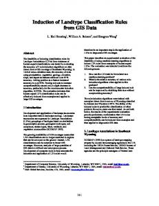
9 Application Domain and Experiment Music Information Retrieval (M IR) is chosen as the application area for our research. In [15], authors present the system MIRAI for automatic indexing of music by instruments and emotions. When MIRAI receives a musical waveform, it divides that waveform into segments of equal size and then its classifiers identify the most dominating musical instruments and emotions associated with each segment and finally with the musical waveform. In [8], [9] authors follow another approach and present a Basic Score Classification Database (BSCD) which describes associations between different scales, regions, genres, and jumps. This database is used to automatically index a piece of music by emotions. In this section, we show how to use action rules extracted from BSCD assuming that we need to change the emotion either from the retrieved or submitted piece of music by minimally changing its score. By a score, in M IR area, we mean a written form of a musical composition. To introduce the problem, let’s start with Figure 2 showing an example of a score of a Pentatonic Minor Scale played in the key of C on a piano. As we can see, 8 notes are played: A], G, A], F, D], G, C and C. The ordered sequence of the same notes without repetitions [A], C, D], F , G] uniquely represents that score. Now, we explain the process of computing its numeric representation [2, 3, 2, 2]. The score is played in the key of A] which becomes the root. Its second note C is 2 tones up from A]. The third note D] is three tones up from C. The fourth note F is two tones up from D], and finally G is two tones up from F . This is how the sequence of jumps [2, 3, 2, 2] with root A] is generated. Essentially any combination of notes A], C, D], F, G can be played while still remaining within the constraints of a C Pentatonic Minor Scale on a piano. This scale is illustrated in Figure 3. Accordingly one plays the root, plays 3 tones up, then 2 tones up then 2 tones up, and then 3 tones up (m means mode). The first note, or in musical terms, the ”Root” is a C note. It means that the remaining four notes are all in the key of C Pentatonic Minor Scale on a piano. However, from the score itself, we have no idea about its key or scale. We can only discern the jumps between the notes and the repeated notes. To tackle the above problem, authors in [8] built a Basic Score Classification Database (BSCD) which describes associations between different scales, regions, genres, and jumps (see Table 4). The attribute Ji means i-th jump. When a music piece is submitted to QAS associated with BSCD, each note one by one, is drawn into the array of incoming signals. Assuming that the score is represented by Figure 2, QAS will generate five optional sequences:
J1 J2 J3 J4 J5 Scale
Region
Genre Emotion
Western
Blues melancholy s
3 2 1 1 2 Blues Major
Western
Blues depressive s
3 2 2 3
Western
Jazz
3 2 1 1 3 Blues Minor
Western
Blues dramatic
s
3 1 3 1 3 Augmented
Western
Jazz
feel-good
s
2 2 2 2 2 Whole Tone
Western
Jazz
push-pull
s
1 2 4 1
Balinese
Balinese
ethnic neutral
s
2 2 3 2
Chinese
Chinese
ethnic neutral
s
2 3 2 3
Egyptian
Egyptian ethnic neutral
s
1 4 1 4
Iwato
Iwato
ethnic neutral
s
1 4 2 1
Japanese
Japanese
Asian neutral
s
2 1 4 1
Hirajoshi
Hirajoshi ethnic neutral
s
1 4 2 1
Kumoi
Japanese
Asian neutral
s
2 2 3 2
Mongolian
Mongolian ethnic neutral
s
1 2 4 3
Pelog
Western
neutral neutral
s
2 2 3 2
Pentatonic Majeur
Western
neutral happy
m
2 3 2 3
Pentatonic 2
Western
neutral neutral
m
3 2 3 2
Pentatonic 3
Western
neutral neutral
m
2 3 2 2
Pentatonic 4
Western
neutral neutral
m
2 2 3 3
Pentatonic Dominant Western
neutral neutral
m
3 2 2 3
Pentatonic Minor
Western
neutral sonorous
m
1 3 3 2
Altered Pentatonic
Western
neutral neutral
m
3 2 1 1 2 Blues
Western
Blues depressive m
4 3
Major
neutral
neutral sonorous
a
3 4
Minor
neutral
neutral sonorous
a
4 3 4
Major 7th Major
neutral
neutral happy
a
4 3 3
Major 7th Minor
neutral
neutral not happy a
3 4 4
Minor 7th Major
neutral
neutral happy
3 4 3
Minor 7th Minor
neutral
neutral not happy a
2 2 3 3
Major 9th
neutral
neutral happy
2 1 4 3
Minor 9th
neutral
neutral not happy a
2 2 1 2 3 Major 11th
neutral
neutral happy
2 1 2 2 3 Minor 11th
neutral
neutral not happy a
4 4
Augmented
neutral
neutral happy
3 3 3
Diminished
neutral
neutral not happy a
2 2 3 2
Pentatonic Major Pentatonic Minor
sma
melancholy s
Table 4. Basic Score Classification Database
a a a a
Fig. 2. Example score of a Pentatonic Minor Scale played in the key of C
Fig. 3. Representation of a Pentatonic Minor Scale
[A], C, D], F , G], [G, A], C, D], F ], [F , G, A], C, D]], [D], F , G, A], C], or [C, D], F , G, A]]. In the first case A] is the root, in the second G is the root, in the third F , in the fourth D], and in the fifth C is the root. Clearly, at this point, QAS has no idea which note is the root and the same which sequence out of the 5 is a representative one for the input sequence of notes A], G, A], F, D], G, C and C. Table 5 gives numeric representation of these five sequences.
Root
J1
J2
J3
J4
]
2
3
2
2
G
3
2
3
2
F
A
2
3
2
3
]
2
2
3
2
C
3
2
2
3
D
Table 5. Possible Representative Jump Sequences for the Input Sequence
Paper [9] presents a heuristic strategy for identifying which sequence out of these five sequences is a representative one for the input score. The same, on the basis of associations between sequences of jumps and emotions which can be extracted from BSCD, we can identify the emotion which invokes in most of us the above input score. What about changes to the input score so the scale associated with that score will change the way user wants. Action rules extracted from BSCD can be used for that purpose and they guarantee the smallest number of changes needed to achieve the goal. Example of an action rule extracted from BSCD is given below: [(J1 , 3 → 2) ? (J2 , 2 → 3)] ⇒ (Scale, P entatonicM inor → Egyptian).
For instance, this rule can be applied to a music score represented by a sequence of 25 notes (Figure 4). They are [A], G, A], C, C, D], D, C, C, F, C, A], C, A], G, A, G, G, D], G, C, D], A], C, C].
Fig. 4. Example of a Music Score
The ordered sequence of the same 25 notes without repetitions [A], C, D, D], F, G] uniquely represents that score. Assume now, that the score is played in the key of G. So, [3, 2, 2, 1, 2] is its numeric representation. The classifier trained on Table 4, based on Levenshtein’s distance [9], identified the sequence [3, 2, 2, 3] as the closest one to [3, 2, 2, 1, 2]. Action rule [(J1 , 3 → 2) ? (J2 , 2 → 3)] ⇒ (Scale, P entatonicM inor → Egyptian)], extracted from Table 4, converts that score to [A], G, A, C, C, D], D, C, C, F, C, A, C, A], G, A, G, G, D], G, C, D], A, C, C]. Please notice that A] is changing to A only if the note C follows it in the input score. This example shows how to use action rules to manipulate the music score. Following the same approach, we can manipulate music emotions, genre, and region.
10 Acknowledgment This material is based in part upon work which was supported by the Ministry of Science and Higher Education in Poland under Grant N N519 404734, Bialystok Technical University under Grant W/WI/2/09, Polish-Japanese Institute of Information Technology under Grant ST/SI/02/08, and by the National Science Foundation under Grant Number IIS-0414815. Any opinions, findings, and conclusions or recommendations expressed in this material are those of the author(s) and do not necessarily reflect the views of the National Science Foundation.
11 Conclusion and Future Work We presented three different algorithms for discovering action rules from a decision table. Rule-based strategies generate less number of action rules than object-based strategies. During the experiment with several data sets, we also noticed that the flexibility of attributes is not equal. For example, the social conditions are less flexible than the health conditions in several data sets used in our experiment, and this fact can be described by
assigning weights to changes of values of attributes. Future work should address this issue jointly with a cost associated with such changes.
References 1. R. Agrawal, R. Srikant (1994), Fast algorithm for mining association rules, Proceeding of the Twentieth International Conference on VLDB, 487-499 2. A. Dardzi´nska, Z. Ra´s (2006), Extracting rules from incomplete decision systems, in Foundations and Novel Approaches in Data Mining, Studies in Computational Intelligence, Vol. 9, Springer, 143-154 3. S. Greco, B. Matarazzo, N. Pappalardo, R. Slowi´nski (2005), Measuring expected effects of interventions based on decision rules, J. Exp. Theor. Artif. Intell., Vol. 17, No. 1-2, 103-118 4. J. Grzymala-Busse (1997), A new version of the rule induction system LERS, Fundamenta Informaticae, Vol. 31, No. 1, 27-39 5. Z. He, X. Xu, S. Deng, R. Ma (2005), Mining action rules from scratch, Expert Systems with Applications, Vol. 29, No. 3, 691-699 6. S. Im, Z.W. Ra´s (2008), Action rule extraction from a decision table: ARED, in Foundations of Intelligent Systems, Proceedings of ISMIS’08, A. An et al. (Eds.), Toronto, Canada, LNAI, Vol. 4994, Springer, 160-168 7. M. Kryszkiewicz (1998), Representative association rules, Proceedings of the Second Pacific-Asia Conference on Research and Development in Knowledge Discovery and Data Mining, LNCS, Vol. 1394, 198-209 8. R. Lewis, Z.W. Ra´s (2007), Rules for processing and manipulating scalar music theory, in Proceedings of the International Conference on Multimedia and Ubiquitous Engineering (MUE 2007), IEEE Computer Society, April 26-28, 2007, in Seoul, South Korea, 819-824 9. R. Lewis, W. Jiang, Z.W. Ra´s (2008), Mining scalar representations in a non-tagged music database, in Foundations of Intelligent Systems, Proceedings of ISMIS’08, A. An et al. (Eds.), Toronto, Canada, LNAI, Vol. 4994, Springer, 445-454 10. C.X. Ling, T. Chen, Q. Yang, Q., J. Chen (2002), Mining optimal actions for intelligent CRM, Proceedings of ICDM0 02, 767-770 11. Z. Pawlak (1981) Information systems - theoretical foundations, Information Systems Journal, Vol. 6, 205-218 12. Y. Qiao, K. Zhong, H.-A. Wang and X. Li (2007), Developing event-condition-action rules in real-time active database, Proceedings of the 2007 ACM symposium on Applied computing, ACM, New York, 511-516 13. Z.W. Ra´s, A. Dardzi´nska (2006), Action rules discovery, a new simplified strategy, Foundations of Intelligent Systems, LNAI, No. 4203, Springer, 445-453 14. Z.W. Ra´s, A. Dardzi´nska, L.-S. Tsay, H. Wasyluk (2008) Association Action Rules, IEEE/ICDM Workshop on Mining Complex Data (MCD 2008), Pisa, Italy, ICDM Workshops Proceedings, IEEE Computer Society, 283-290 15. Z.W. Ras, X. Zhang, R. Lewis (2007), MIRAI: Multi-hierarchical, FS-tree based music information retrieval system, (Invited Paper), in Proceedings of RSEISP 2007”, LNAI, Vol. 4585, Springer, 80-89 16. Z.W. Ra´s, A. Wieczorkowska (2000), Action-Rules: How to increase profit of a company, in Principles of Data Mining and Knowledge Discovery, Proceedings of PKDD 2000, Lyon, France, LNAI, No. 1910, Springer, 587-592 17. Z. Ra´s, E. Wyrzykowska, H. Wasyluk (2008), ARAS: Action rules discovery based on agglomerative strategy, in Mining Complex Data, Post-Proceedings of 2007 ECML/PKDD Third International Workshop (MCD 2007), LNAI, Vol. 4944, Springer, 196-208
18. L.-S. Tsay, Z.W. Ra´s (2005) Action rules discovery: system DEAR2, method and experiments, Journal of Experimental and Theoretical Artificial Intelligence, Taylor and Francis, Vol. 17, No. 1-2, 119-128 19. A. Tzacheva, Z.W. Ra´s (2007), Constraint based action rule discovery with single classification rules, in Proceedings of the Joint Rough Sets Symposium (JRS07), LNAI, Vol. 4482, Springer, 322-329 20. A. Tzacheva, Z.W. Ra´s (2005) Action rules mining, International Journal of Intelligent Systems, Wiley, Vol. 20, No. 7, 719-736 21. Q. Yang, H. Chen (2002) Mining case for action recommendation, Proceedings of ICDM0 02, 2002, 522-529 22. Q. Yang, J. Yin, C.X. Lin, T. Chen (2003) Postprocessing decision trees to extract actionable knowledge, Proceedings of ICDM0 03, 685-688 23. K. Wang, Y. Jiang, A. Tuzhilin (2006) Mining actionable patterns by role models, Proceedings of the 22nd International Conference on Data Engineering, 3-7 April, 2006, 16-26 24. H. Zhang, Y. Zhao, L. Cao, C. Zhang (2008), Combined association rule mining, in Advances in Knowledge Discovery and Data Mining, Proceedings of the PAKDD Conference, LNCS, No. 5012, Springer, 1069-1074