Modulus б Compliance б Creep б .... The standard definition of a relaxation spectrum is used and a relaxation .... the meaning of the steady-state compliance.
Rheol Acta (2001) 40: 261±271 Ó Springer-Verlag 2001
Alexander Ya. Malkin Irima Masalova
Received: 15 March 2000 Accepted: 18 September 2000
A. Ya. Malkin á I. Masalova Cape Technikon, Engineering Faculty Department of Civil Engineering PO Box 652, Cape Town 8000 Republic of South Africa A. Ya. Malkin (&) Research Institute for Plastics Profsoyuznaya 98, korp.5, kv. 92 Moscow, 117485, Russia e-mail: alex@malkin. msk.ru
ORIGINAL CONTRIBUTION
From dynamic modulus via different relaxation spectra to relaxation and creep functions
Abstract The main goal of the paper is to compare predictive power of relaxation spectra found by dierent methods of calculations. The experimental data were obtained for a new family of propylene random copolymers with 1-pentene as a comonomer. The results of measurements include ¯ow curves, viscoelastic properties, creep curves and rubbery elasticity of copolymer melts. Dierent relaxation spectra were calculated using independent methods based on dierent ideas. It lead to various distributions of relaxation times and their ``weights''. However, all of them correctly describe the frequency dependencies of dynamic modulus. Besides, calculated spectra were used for ®nding integral characteristics of viscoelastic behaviour of a material (Newtonian viscosity, the normal stress coecient, steadystate compliance). In this sense all approaches are equivalent, though it appears impossible to estimate instantaneous modulus. The most crucial arguments in estimating the results of dierent approaches is calculating the other viscoelastic function and predicting behaviour of a material in various deformation modes. It is the relax-
Introduction The title of the paper completely represents its purpose and the key word is ``dierent''. It is only necessary to
ation and creep functions. The results of relaxation curve calculations show that all methods used give rather similar results in the central part of the curves, but the relaxation curves begin to diverge when approaching the high-time (low-frequency) boundary of the relaxation curves. The distributions of retardation times calculated through dierent approaches also appear very dierent. Meanwhile, predictions of the creep curves based on these dierent retardation spectra are rather close to each other and coincide with the experimental points in the wide time range. Relatively slight divergences are observed close to the upper boundary of the experimental window. All these results support the conclusion about a rather free choice of the relaxation time spectrum in ®tting experimental data and predicting viscoelastic behaviour of a material in dierent deformation modes. Key words Rheology á Polypropylene á Copolymers á Shear viscosity á Flow curve á Relaxation spectrum á Rubbery elasticity á Modulus á Compliance á Creep á Approximation methods
add the question: does the ®nal result depend on the choice of a spectrum? This question does not have a trivial answer. Certainly, well known rigorous theoretical equations connect the functions referred in the title
262
(see, e.g. Gross 1953; Ferry 1980; Tschoegl 1989). However, one deals with not exactly de®ned values, with experimental data which are always obtained with a certain error and the whole discussion takes place in the ®eld of approximations. Then, several nonlinear operations take place in treating initial experimental data and the problem becomes ill-de®ned or incorrect by its nature (Honerkamp and Weese 1989, 1990, 1993; Malkin 1990). There are a lot of papers (see, e.g. Baumgaertel and Winter 1989, 1992; Emri and Tschoegl 1993, 1997; Tschoegl and Emri 1993; Dooling et al. 1997; Kaschta and Schwarzl 1994; Elster at al. 1991; Orbey and Dealy 1991; Elster and Honerkamp 1992; Malkin 1996; Malkin and Kuznetsov 2000; Roths et al. 2000) devoted to calculations of a relaxation spectrum basing on experimentally found frequency dependencies of the components of dynamic modulus, G¢(x) and G¢¢(x). The ®nal results of numerous attempts to ®nd the ``true'' relaxation spectrum was summarised in the following way: the problem of line spectrum determination is essentially a curve ®tting procedure and ``no line spectrum ± produced by whatever method ± is ever the true spectrum'' (Tschoegl and Emri 1993). Besides, Winter (1997) concludes that the choice of an algorithm for determining a relaxation spectrum is ``personal preference rather than objective de®nition''. Meanwhile, it is expected that a relaxation spectrum, found in this or that way, must not only be adequate for initial experimental data but also have predictive power and allow one to describe other viscoelastic functions, primarily relaxation and creep curves. It was demonstrated (Malkin 1990) that, generally speaking, the results of such predictions can be poor even if the relaxation spectrum corresponds to initial experimental data for G¢(x) and G¢¢(x). The purpose of this article is to present new experimental data and the results of calculations related to this problem.
Experimental Samples The subject of this study was polypropylene and random copolymers of propylene with 1-pentene. Some results of rheological studies of propylene/1-pentene random copolymers were ®rst published by Halasz et al. (1998). Copolymers were produced in a heptene slurry using two dierent catalysts of the Zigler-Natta type at the temperatures between 20 °C and 80 °C. The list of main samples used, their designations and principle characteristics are summarised in Table 1. All samples have a rather wide molecular weight distribution: it � n lies � w =M was reported that for the majority of samples the ratio M in the range 5.5 0.5.
Table 1 Main sample used and their principal characteristics Sample
Structure
� n 10)3 M
� w 10)3 M
MFI at 190 °C
PP-1 COP-2 COP-3 COP-4
Homo 0.96%pentene 2.0%pentene 4.9%pentene
480 530 650 710
88 100 125 110
7.0 6.7 5.7 5.3
Instrumentation The rheological measurements were carried out using a stress controlled Rheometrics SR 500 instrument. The measuring head was a parallel plate unit with diameter 2.5 mm and a gap of 1 mm. All experiments were repeated using a 4.0-mm disk measuring head, and the obtained results were quite reproducible. Three dierent regimes of deformation were used: ± Steady state ¯ow for measuring ¯ow curves (apparent viscosity vs shear rate) ± Oscillatory (dynamic) measurements for measuring frequency dependencies of the (storage and loss) components of dynamic modulus measured in a wide range of frequencies ± Unsteady creep at constant shear stress and elastic recovery after sudden cessation of loading All rheological measurements were made in the temperature range 190±230 °C. In utilising the experimental results and approximating them by the dierent ®tting equations, a standard software ± MatLab ± was used.
Experimental results There is no need to demonstrate here the initial experimental data for ¯ow curves, temperature dependencies of viscosity, and G¢(x) and G¢¢(x) dependencies, because they look quite trivial and basically are the same as described for numerous polymer melts. Only some of the important experimental results will be cited below. First, ¯ow curves for all samples can be described by the Carreau equation (Carreau 1972) and its constants were found by the computer-aided ®tting g _ n N 1
kc
1 g0 where g0 is, as usual, zero-shear-rate (Newtonian) viscosity, k is a characteristic Carreau-relaxation time, and n and N are the empirical power exponents of the model, and their ratio is 0.7 0.1 for all samples studied in this work. The parameters of this equation were found in the following manner: ®rst the ratio n/N was found from the power-law part of the curve and g0 was measured in the Newtonian branch of the ¯ow curve, then other constants were determined by the standard mean-least-square procedure. Second, Newtonian viscosity, g0, was found by three methods: from ®tting experimental ¯ow curves by Eq. (1), from the results of the dynamic measurements in the range of low frequencies G¢¢ � G¢ as lim(G¢¢/x) at
263
x ® 0, and from creep experiment. In all cases the obtained values of g0 correlate quite well with each other. The limits of experimental error were estimated as 5%. Third, the coecient of normal stresses (or more exactly the coecient of the ®rst dierence of normal � stresses) V0, de®ned as lim N1 =2c_ 2 at c_ ! 0; was not measured directly but found through the following methods: 1. It was proven (Vinogradov and Malkin 1980, p 282) that, in the limit of zero frequency, assuming that G¢¢ � G¢, G0 ; x!0 x2
10 lim
2
2. The second method used for calculation of the normal stress coecient is based on the rigorously obtained relationship (Malkin 1971): Z1 2 dg
c_
3 10 p c_ 0
which is close (by its structure) to the so-named ``mirror relation'' proposed by Gleissle (1982). In his case the pre-integral coecient is equal not to 2/p » 0.64 but to 0.5, the dierence being immaterial 3. It was shown (Vinogradov and Malkin 1980) that there is correlation between the ¯ow curve and the coecient V0. If the ¯ow curve is presented by Eq. (1), then this correlation is expressed be the formula 10 Kkg0
4
and the numerical value of the coecient K lies between 0.2 and 0.3 (let it be 0.25 for further calculations). The application of any of these methods gives rather close results and it allowed us to ®nd the values of V0 with the error not exceeding 20%. Fourth, steady-state compliance, I0e , was determined directly through measuring elastic recoil after sudden cessation of loading: c Ie0 el
5 s where cel is the elastic (reversible) deformation at shear stress s. Besides, it is possible to compare the values of I0e found directly by Eq. (5) and calculated from quantities determined above. Indeed, it is possible to calculate I0e by the two following methods. 1. The following very well known relationship can be used for calculating I0e : 1 Ie0 02
6 g0
2. It is possible to use the results of dynamic measurements and ®nd I0e as Ie0 lim
G0
x!0
G00 2
;
7
Comparison of the values of I0e calculated from Eq. (5) ± i.e. found directly ± and Eqs. (6) and (7) ± i.e. by indirect methods ± demonstrates that there is a very close correlation among the results of calculations made by dierent methods. Fifth, characteristic relaxation time, h0, were also found, h0 being de®ned as h0
df0 g0
8
So, the value of h0 is not an independent characteristic of the rheological properties of a material but is determined by two other independent parameters, g0 and f0. However, the parameter h0 is useful for comparison of dierent polymers. The interesting aspect in calculating h0 is related to comparison between h0 and the Carreau relaxation time, k, found in ®tting the experimental ¯ow curves by Eq. (1). This is done in Fig. 1, where all points are collected. It is seen that there is a linear correlation between h0 and k expressed by the relationship k Ah0
9
where A 3.84. This result (as well as the equations for the normal stress coecient) demonstrates that a very close relationship between non-Newtonian and viscoelastic properties of a polymer melts exists.
Fig. 1 Correlation between the characteristic relaxation time found in oscillatory experiments, h0 and the Carreau relaxation time, k
264
Sixth, frequency dependencies of both components of the dynamic modulus, G¢ and G¢¢ were measured in the log frequency (in s)1) range from )1.5 to 2.0. The detailed discussion of these data appears below. Here, it is worth mentioning that the values of both modulus components at the crossover point, Gc, appear rather close to each other, and Gc for all samples under investigation is equal to 25 5 kPa. Seventh, creep functions were measured in the linear range of viscoelastic behaviour. Linearity was checked using the standard method: independence of the measured curves was observed in fourfold changing of stress applied.
Relaxation spectra As was discussed in the introduction, there is an unlimited number of relaxation spectra which are adequate for measured (in limited experimental window) G¢(x) and G¢¢(x) dependencies. Meanwhile, the requirement for correspondence of G¢(x) and G¢¢(x), calculated from a relaxation spectra, to experimental data is provision of the required (but probably inadequate) conditions. The standard de®nition of a relaxation spectrum is used and a relaxation spectrum is treated as discrete. As is well known, a relaxation spectrum is related to the frequency dependencies of the storage, G¢(x), and loss, G¢¢(x), components of dynamic modulus as N X
xsn 2 G0
x gn
10 1
xsn 2 n1
G00
x
N X n1
gn
xsn
1
xsn 2
11
where gn is the ``weight'' of the n-th line of a relaxation spectrum at the corresponding argument values ± relaxation times sn ± and N is the total number of lines (discrete relaxation times). Four dierent procedures for search for the parameters of a relaxation spectrum were chosen. Method A ± the ®rst method is based on the idea of the equidistant distribution of relaxation times along the log-frequency range. Let the experimental widow be xmin ) xmax, or 1 1 xmax ) xmin in reciprocal units. According to the recommendation of Winter (1997) this interval was widened by including an additional frequency decade on both sides. Then this broad frequency scale is divided into several equal intervals in a log scale. It is assumed that the middle of every logarithmic interval is equal to a relaxation time sn. In the procedure described above the relaxation times distribution is expressed as
log sn log smax Cn
12 where n is the number of a relaxation mode and C is the step. Method B ± in this approximation the distribution of relaxation times is supposed to be in the power law form: sn 3smax =n a
13 )1 where the initial value of smax is determined as 5x . The factor 5 means that the maximal relaxation time is shifted beyond the boundaries of the experimental window. Here the number of a mode n is changing from 1 to N, and N is the total number of relaxation modes. This power-type distribution in this approach is quite arbitrary. It is close to the physically based distribution discussed in the Doi and Edwards (1986) model. However the power value assumed in Eq. (13) is much higher than obtained in their work. Method C ± the method of linearisation of functional of errors was proposed by Malkin(1996) and Malkin and Kuznetsov (2000). This method consists essentially of presenting the experimentally found frequency dependencies of the component of dynamic modulus in the form of a power series and searching for the coecients of this series by the minimising least-root-square-error using the computer-aided procedure. Method D ± in this work a non-linear method, proposed by Baumgaertel and Winter (1989, 1992) and Winter (1997) ± the so-called IRIS method ± was also used. The standard procedure of minimisation of the meansquare-root error in any approximation was used. This procedure takes into account the results of measurements of G¢ and G¢¢ in all experimental points. In this case an averaged error, X, is calculated as v u 2 !2 !3 2 uX 0 0 00 00 N G G G G u 1 exp;n cal;n exp;n cal;n 5 t 4 E 2N N 1 G0exp;n G00exp;n
14 where G¢exp,n(xn) and G¢¢exp,n(xn) are experimental values of G¢ and G¢¢ at several points, xn, along the frequency scale; G¢cal,n(xn) and G¢¢cal,n(xn) are calculated values of G¢ and G¢¢ at the same frequency points, xn, which are found from gi and si values, that is, it is relaxation spectrum lines approximating the experimental data. According to Methods A and B, values of sn are known (set beforehand) and the gn values are found by minimising E. According to Methods C and D, values of both gn and sn must be found by minimising E, either by the linear Method C or the non-linear Method D. This standard and rather evident estimation of E has a principal disadvantage: it does not allows one to control the errors of approximations on the dierent
265
argument intervals. Meanwhile, their input can play a dierent role with the dierent intervals. An attempt to improve the situation leads to the idea of using the so-called ``weighted'' mean-square-root-error method. In this approach the averaged error is calculated as
and f0
N X n1
s2n gn
18
It appeared that satisfactory approximation of the
v u 2 !2 � � !2 � � 3 experimental curves was reached in all cases, as it was uX 0 0 00 00 a1 a2 N Gexp;n Gcal;n Gexp;n Gcal;n 1u x0 x0 5 the basic necessary condition in searching a relaxation E t 4 xn xn 2N N1 G0exp;n G00exp;n spectrum. The reverse calculations of the frequency
15 Here the weights 1/xna1 and 1/xna2 are introduced in order to improve the approximation for the particular intervals of a frequency scale, and x0 is a normalising factor; its exact value is immaterial because it is introduced only to make the correcting frequency, xn, dimensionless. In this work x0 was assumed to be equal to 1 s)1. If a > 0, the importance of the low frequency region is increased, while for a