to the haptic feeling of fabric. P. Volino*, P. Davy*, U. Bonanni*, N. Magnenat-Thalmann*. G. Böttcher**, D. Allerkamp**, F.-E. Wolter**. * MIRALab - University of ...
From measured physical parameters to the haptic feeling of fabric P. Volino*, P. Davy*, U. Bonanni*, N. Magnenat-Thalmann* G. Böttcher**, D. Allerkamp**, F.-E. Wolter** * MIRALab - University of Geneva ** Welfenlab - University of Hanover
Abstract Real-time cloth simulation involves many computational challenges to be solved, particularly in the context of haptic applications, where high frame rates are necessary for obtaining a satisfactory tactile experience.In this paper, we present a realtime cloth simulation system which offers a compromise between a realistic physicallybased simulation of fabrics and a haptic application with high requirements in terms of computation speed. We give emphasis on architecture and algorithmic choices for obtaining the best compromise in the context of haptic applications. A first implementation using a haptic device demonstrates the features of the proposed system and leads to the development of new approaches for the haptic rendering using the proposed approach. Keywords: haptics, force feedback, real-time, cloth-simulation, elastic deformation
1. Introduction A key factor for achieving convincing haptic interaction is the successful integration of realistic graphical rendering and adequate haptic rendering techniques. If the haptic interaction occurs with deformable objects belonging to everyday life, the simulation accuracy of the object’s behavior plays a fundamental role, and physically-based simulation is necessary. At first glance, the advantage of physically-based simulation in the context of haptics seems obvious: The mechanical models driving the visual simulation could easily be used for computing the resulting forces for the haptic rendering in a direct way. However, the graphics rendering loop has different
requirements compared to the haptic rendering loop in terms of refresh frequencies. While in graphics a refresh rate of 30 fps is quite acceptable, in haptics a response frequency of 300-1000 Hz is needed to ensure accurate interaction. For this reason, a good approach for the development of Virtual Reality (VR) Systems for the visual and haptic rendering of deformable objects is to consider a multi-layer architecture for what concerns the physical-based models driving the simulation [1]. The first layer consists of a coarse model representing the large-scale features of the deformable object (for the graphics rendering), while the second layer is a finer local model defining the surface characteristics close to the point of interaction dedicated to meet the haptic requirement. This paper presents the visual and haptic rendering techniques proposed in the context of the HAPTEX Project, which aims at developing a Virtual Reality System for the multimodal perception of textiles [2]. The aim of the project is to reproduce the feeling of touching a cloth surface with two fingertips, simulating both the large-scale motion of a square of fabric accurately described by its mechanical properties (strain-stress curves), and the small scale properties (texture and roughness) for the tactile perception. In this paper, we will first examine the related work for this area with an emphasis on the way to measure the physical parameters. Then, the large-scale mechanical model simulating the macroscopic deformation of cloth will be presented. Finally, a first implementation of haptic interaction model will be presented.
2. Related Work 2.1 Understanding and Properties of Fabrics
Modeling
the
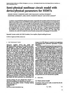
The process of handling fabrics to understand their properties and structure is called “fabric hand” [3]. Modeling the behavior of textiles is a complex task because of its dependency on several parameters such as flexibility, compressibility, elasticity, resilience, density, surface contour (roughness, smoothness), surface friction and thermal character [4]. For the large scale simulation, fabrics are approximated as thin 2D surfaces, thus we can avoid taking into consideration pressurethickness, surface friction and surface roughness. However, we can use objective measurement methods to acquire other parameters such as tensile, shearing or bending variables. An objective assessment of the fabric hand is achieved through hardware equipments, such as tensile testers or the Kawabata measurement systems. These equipments are able to test for textile properties and extract the strain-stress curves for weft and warp elongation, shear deformation, bending, pressure-thickness, surface friction and surface roughness. The values of the extracted parameters vary depending on the fiber type or fabric type and dimension. The data obtained from measurements on fabrics serves as an input to the mechanical model driving our cloth simulation system.
Figure 1: Strain stress curve from Kawabata tensile test
An interesting consideration at this point is the possibility to go also in the opposite direction: through the use of an accurate cloth simulation scheme it is also possible to study new fabrics. We can develop and model non-
existing textiles, which look and behave in a realistic way and have specific properties. Such virtual textiles would not base on any “real” counterparts, but could be produced by the textile industries after successful simulation. 2.2 Cloth Simulation In computer graphics, cloth objects are represented by polygonal meshes. During cloth animation, the vertices of the cloth mesh are driven by the laws of the underlying physical model. The resulting equations are solved using numerical methods such as the semi-implicit Backward Euler method, which was first used by Baraff et al. [5] in the context of cloth simulation. Since then, semiimplicit integration has been widely used for cloth animation, as it provides better results in terms of stability and speed compared to other integration schemes [6]. An exhaustive overview of the state of the art in cloth animation research is given by [7]. In recent years, several research activities have been carried on in the field of cloth simulation, focusing on different aspects ranging from physical based models [8], [9] to integration schemes [5], [10] and collision response [11], [12]. In the following, we briefly describe existing simulation schemes underlying mechanical models for cloth simulation. 2.2.1. Continuum Mechanics
In another approach, mechanical equations of continuum mechanics are expressed along the curved surface, and then discretized for their numerical resolution. Such accurate schemes are however slow and not sufficiently versatile for handling large deformations and complex geometrical constraints (collisions) properly. Finite Element methods express the mechanical equations according to the deformation state of the surface within welldefined elements (usually triangular or quadrangular). Their resolution also involves large computational costs [13]. Another option is to construct a model based on the interaction of neighboring discrete points of the surface. Such particle systems allow the implementation of simple and versatile models adapted for efficient computation of highly deformable objects such as cloth.
Bending Deformation
2.2.2. Spring-Mass Models
The simplest particle system one can think of is a spring-mass system. In this scheme, the only interactions are forces exerted between neighboring particle couples, similarly as if they were attached by springs (described by a force/elongation law along its direction, which is actually a rigidity coefficient and a rest length in the case of linear springs) [14]. Spring-mass schemes are very popular methods, as they allow simple implementation and fast simulation of cloth objects. There has also been recent interest in this method as it allows quite a simple computation of the Jacobian of the spring forces, which is needed for implementing semi-implicit integration methods. The simplest approach is to construct the springs along the edges of a triangular mesh describing the surface. This however leads to a very inaccurate model that cannot describe accurately the anisotropic strain-stress behavior of the cloth material, and also not the bending. More accurate models are constructed on regular square particle grids describing the surface. While elongation stiffness is modeled by springs along the edges of the grid, shear stiffness is modeled by diagonal springs and bending stiffness is modeled by leapfrog spring along the edges (Figure 2). This model is still fairly inaccurate because of the unavoidable crossdependencies between the various deformation modes relatively to the corresponding springs. It is also inappropriate for nonlinear elastic models and large deformations. More accurate variations of the model consider angular springs rather than straight springs for representing shear and bending stiffness, but the simplicity of the original spring-mass scheme is then lost. The model detailed in Part 3 alleviates these issues by combining the simplicity and speed of particle systems with the accuracy of a model that evaluates strain and stress on the true deformed surface of cloth.
Shearing Deformation Length
Metric Deformation
Length Length
Angle Angle
Figure 2: Using length or angle springs for simulating cloth with a square particle system grid.
2.3 Toward Haptic Rendering of Textiles Haptic Rendering algorithms are responsible for reproducing the forces acting on the simulated objects and transmit them to the haptic interface. In the case of static, non deformable objects, the computation of these forces is limited to reproducing the object’s stiffness according to the user’s position and interaction speed. When simulating dynamic deformable surfaces such as textiles, however, this issue grows in complexity, as the simulated surface has its own behavior which influences the haptic feedback and therefore has to be taken into consideration. There has been very little research on the haptic rendering of textiles so far [15] [16] [17]. In all cases, projects dealing with haptic perception of textiles targeted very specific scenarios and were severly limited in terms of visual rendering (no real-time animation), used hardware (low-cost commercial products or expensive ad-hoc devices) or targeted realism (static, non deformable textiles). A system which provides both force feedback and tactile perception of virtual textiles through a haptic device, and is synchronized with a real-time, physical based graphical simulation of the fabric has still not been developed yet. To achieve this challenging goal, several advances in all related fields are necessary: from the techniques of fabric measurements, to the development of novel haptic devices and the improvement of physical-based models for real-time cloth simulation.
3. A Mechanical Model for RealTime Cloth Simulation 3.1. Key Techniques for Real-Time Cloth Simulation The most important challenge is to simulate in real-time cloth materials which are accurately described by nonlinear anisotropic
mechanical models (weft, warp and shear strain-stress curves). Most existing real-time simulation systems consider drastic simplifications in the mechanical model (isotropic linear elasticity) and even change the mechanical nature of the material (for example, reduce stiffness by simulating very deformable materials) for getting more computation speed. However, our application requires the simulation of precise mechanical behavior of cloth. Going away from traditional grid-based spring-mass approaches, we propose a very accurate particle system which reaches the accuracy of first-order nonlinear finite elements while retaining the simplicity of particle systems. This model uses a fast computational method for evaluating precisely the strain state of a triangle of the cloth surfaces, and may then turn the corresponding stress back into particle forces. Real-time constraints however impose a severely limited complexity of the mechanical system. Here are the main simplifications that we consider: y Simulation of a coarse grid, typically limited to a thousand of triangle elements. What matters for the computation time is not only the number of elements to be computed, but also the size of these elements (the smaller they are, the stiffer the numerical system will be). y Neglecting bending stiffness. Bending stiffness is usually very low in usual fabric materials, and it usually does not make any sense simulating bending effects producing millimeter wrinkles with centimeter mesh elements. Bending properties are also quite costly to compute. y Not performing self-collision within the cloth. Self-collision techniques are usually quite costly in computational resources, and processing the detected collisions is also complex. Given the simple context of our animation (a hanging piece of cloth), we restrict collision processing to detecting contacts between the cloth object and the haptic virtual fingertips. Large simulation time steps should be considered for the numerical integration of the system, and this is obtained through the use of implicit numerical integration methods. This however slightly alters the dynamic behavior of the cloth (numerical
damping). Experimental tests can help finding the best time-steps producing animation of cloth objects with damping in par with the damping observed in real cloth materials. 3.2. Mechanical Modeling of Cloth The mechanical behavior of cloth (approximated as a thin surface) is decomposed in in-plane deformations (the 2D deformations along the cloth surface plane) and bending deformation (the 3D surface curvature). The tensile behavior of cloth is described by relationships relating, for any cloth element, the stress σ to the strain ε (for elasticity) and its speed ε' (for viscosity) according to the laws of viscoelasticity. For cloth materials, strain and stress are described relatively to the weave directions weft and warp following three components: weft and warp elongation (uu and vv), and shear (uv). Thus, the general viscoelastic behavior of a cloth element is described by strain-stress relationships as follows: σ uu (ε uu , ε vv , ε uv , ε uu ′ , ε vv′ , ε uv′ ) σ vv (ε uu , ε vv , ε uv , ε uu ′ , ε vv′ , ε uv′ ) σ uv (ε uu , ε vv , ε uv , ε uu ′ , ε vv′ , ε uv′ )
Assuming to deal with an orthotropic material (usually resulting from the symmetry of the cloth weave structure relatively to the weave directions), there is no dependency between the elongation components (uu and vv) and the shear component (uv). Assuming null Poisson coefficient as well (a rough approximation), all components are independent, and the fabric elasticity is simply described by three independent elastic strain-stress curves σuu(εuu), σvv(εvv), σuv(εuv) (weft, warp, shear), along with their possible viscosity counterparts. In the same manner, viscoelastic strain-stress relationships relate the bending momentum to the surface curvature for weft, warp and shear. With the typical approximations used with cloth materials, the elastic laws are only two independent curves along weft and warp directions (shear is neglected), with their possible viscosity counterparts.
(1)
3.3. A Fast and Accurate Particle System Model Our initial goal is to design an efficient mechanical simulation scheme for simulating the large-scale behavior of the cloth. Because of the real need of representing accurately the anisotropic nonlinear mechanical behavior of cloth in applications, spring-mass models are inadequate, and we need to find out a scheme that really simulates the viscoelastic behavior of actual surfaces. For this, we have defined a particle system model that relates this accurately over any arbitrary cloth triangle through simultaneous interaction between the three particles which are the triangle vertices. Such a model integrates directly and accurately any strainstress model using polynomial spline approximations of the strain-stress curves, and remains accurate for large deformations. Details on this approximation of strain-stress curves are given in appendix A.2. 3.3.1. Assumptions
Cloth is typically represented by curved surfaces composed of polygonal meshes, being either triangular or quadrangular, and regular or irregular. In order to enrich these geometrical surfaces with the above mentioned mechanical properties, we need to define a specific mechanical model. We consider the following constraints for designing the large-scale simulation system: • The geometrical description of the cloth surface should be any triangular mesh. • The mechanical properties of the cloth material is described by strain-stress curves, approximated analytically as independent piece-wise polynomial splines (weft, warp, shear). • Bending stiffness is neglected, as it does not make sense to spend time computing accurately their very weak effect comparatively to the scale required for real-time simulation of the model (the size of the elements are much more likely to limit the sharpness of the wrinkle patterns than the bending stiffness of the cloth). 3.3.2. Description of the Model
In this model, a triangle element of cloth is described by 3 2D coordinates (ua, va), (ub, vb), (uc, vc) describing the location of its vertices A, B, C on the weft-warp coordinate
system defined by the directions U and V with an arbitrary origin. They are orthonormal on the undeformed cloth (figure 2). Out of them, a pre-computation process evaluates the following values: Rua = d −1 (vb − vc )
Rva = −d −1 (ub − uc )
Rub = −d −1 (va − vc )
Rvb = d −1 (ua − uc )
Ruc = d −1 (va − vb )
Rvc = −d −1 (ua − ub )
with d = ua (vb − vc ) + ub (vc − va ) + uc (va − vb )
(2)
During the computation process, the current deformation state of the cloth triangle is evaluated using the current 3D direction and length of the deformed weft and warp direction vectors U and V. They are computed from the current positions Pa, Pb, Pc of its supporting vertices as follows: U = Rua Pa + Rub Pb + Ruc Pc V = Rva Pa + Rvb Pb + Rvc Pc
(3)
The current in-plane strains ε of the cloth triangle is then computed with the following formula: ε uu = U − 1 ε uv =
ε vv = V − 1
U +V
−
2
(4)
U −V 2
We have chosen to replace the traditional shear deformation evaluation based on the angle measurement between the thread directions by an evaluation based on the length of the diagonal directions. The main advantage of this is a better accuracy for large deformations (the computation of the behavior of an isotropic material under large deformations remains more axisindependent). Ruc Rvc
Pa Pc
V U
V U v
y Rua Rva
u in Fabric Coordinates Definition
V U
z Pb
Rub Rvb
x Deformation in World Coordinates
Deformed fabric triangle
Figure 3: A triangle of cloth element defined on the 2D cloth surface (left) is deformed in 3D space (center) and its deformation state is computed from the deformation of its weft-warp coordinate system (right).
For applications that model internal in-plane viscosity of the material, the "evolution speeds" of the weave direction vectors are needed as well. They are computed from the
current triangle vertex speeds Pa', Pb', Pc' as follows: U ′ = Rua Pa′ + Rub Pb′ + Ruc Pc′
(5)
V ′ = Rva Pa′ + Rvb Pb′ + Rvc Pc′
Then, the current in-plane strain speeds ε' of the triangle is computed: ε uu′ =
U ⋅U ′ U
ε vv′ =
V ⋅V′ V
(6)
(U + V )⋅ (U ′ + V ′ ) − (U − V )⋅ (U ′ − V ′ ) ε uv′ = U +V
2
U −V
2
At this point, the in-plane mechanical behavior of the material can be expressed for computing the stresses σ out of the strains ε (elasticity) and the strain speeds ε' (viscosity) using the curves (1). Finally, the force contributions of the cloth triangle to its support vertices computed from the stresses σ as follows: d⎛ U V⎞ Fa = − ⎜ (Rua σ uu + Rva σ uv ) + (Rua σ uv + Rva σ vv ) ⎟ 2⎝ U V⎠ Fb = −
d⎛ U V⎞ (Rub σ uu + Rvb σ uv ) + (Rub σ uv + Rvb σ vv ) ⎟ 2 ⎜⎝ U V⎠
Fc = −
d⎛ U V⎞ (Ruc σ uu + Rvc σ uv ) + (Ruc σ uv + Rvc σ vv ) ⎟ 2 ⎜⎝ U V⎠
It is important to note that when using semiimplicit integration schemes, the contribution of these forces in the Jacobian ∂F/∂P and ∂F/∂P' can easily be computed out of the curve derivatives ∂σ/∂ε and the orientation of the vectors U and V. 3.3.3. Numerical Integration
The equations resulting from the mechanical formulation of particle systems do usually express particle forces F depending on the state of the system (particle positions P and speeds P'). In turn, particle accelerations P" is related to particle forces F and masses M by Newton's 2nd law of dynamics. This leads to a second-order ordinary differential equation system, which is turned to firstorder by concatenation of particle position P and speed P' into a state vector Q. Some details about how the differential equation system is set are given in appendix A.1. A vast range of numerical methods has been studied for solving this kind of equations. The most widely-used method for cloth simulation is currently the semi-implicit Backward Euler method, which was first used by Baraff et al. [5] in the context of cloth simulation. As any implicit method, it
alleviates the need of high accuracy for the simulation of stiff differential equations, offering convergence for large timesteps rather than numerical instability (a step of the semi-implicit Euler method with "infinite" timestep is actually equivalent to an iteration of the Newton resolution method) [6]. Many variations of this method are available, through various computational simplification approaches [18][19][8]. The formulation of a generalized implicit Euler integration is the following: Q(t +dt ) − Q(t ) = Q(t′ +α dt) dt
(8)
The derivative value is not known at a moment after t, and is then extrapolated from the value at moment t using the Jacobian, leading to the semi-implicit expression which requires the resolution of a linear system: (7)
⎛ ⎞ ∂Q ′ Q(t +dt ) − Q(t ) = ⎜ I − α dt ⎟ ∂Q (t ) ⎠ ⎝
−1
Q(t′ ) dt
We have introduced the coefficient α so as to modulate the "impliciticy" of the formula[20]. Hence, α = 1 is the regular implicit Backward Euler step (stable), whereas α = 0 is the explicit Forward Euler step (unstable), and α = 1/2 is the 2nd-order implicit Midpoint step (most accurate, at the threshold of stability). The α parameter is a good handle for adjusting the compromise between stability and accuracy. While maximum robustness is obviously observed for large values, reducing its value increases accuracy (reduces numerical damping) at the expense of stability, and speeds up the computation as well (better conditioning of the linear system to be resolved). Hence, for our real-time application, we can modulate this value according to the simulation and interaction requirements to offer the best accuracy and robustness. The requirement of high robustness of haptic applications also makes higherorder methods [21] [10] less adequate. 3.4. Collision Processing Due to constraints for real-time performance, self-collision detection on the cloth object is ignored. The only task in this field is to detect collisions between solid objects and the cloth surface. This task is performed through an adapted bounding-volume hierarchy
(9)
algorithm, which uses a constant DiscreteOrientation-Polytope hierarchy constructed on the mesh [12] [22]. The solid object is itself embedded in a polytope, and collision detection is done through traversal of the colliding nodes of the hierarchy.
sent from the model. A point based interaction is currently considered. The force is calculated by detecting and generating responses for the collision between the haptic cursor and the surface.
4. Haptic Rendering
To detect the collision between the surface and the haptic cursor, a global coarse level collision is computed as described in section 3.4, then the exact collision is computed for the set of triangles in the selected bounding box. At the moment when a collision occurs, the HIP (Haptic Interface Point) is penetrating the surface and the IHIP (Ideal Haptic Interface Point) is forced to stay on the surface. Then the force sent to the haptic device is calculated based on the relative position of the HIP and the IHIP, as it can be seen on figure 5. It can be computed from the laws of Hooke and Coulomb[23].
A first implementation of haptic simulation has shown a few limitations. Due to the bidirectional nature of haptic, adding its support can lead to considerations on two different forces. First, in section 4.1 we present the method used to send the force to the user. Then, in section 4.3. we discuss the forces sent to the mechanical model. Furthermore one of the main issues in haptic rendering is to find a solution for the problem of different update rates. Indeed, the user communicates with the virtual environment through a probe, the “haptic cursor”. This cursor is used to transmit forces to the surface and to the user. A high update rate of forces (1 kHz) is needed to give the user a satisfying experience of touch and feel of virtual objects. Since the simulation of the mechanics being synchronized with the visual rendering loop runs at a much lower frequency (