From median filters to optimal stack filtering - Circuits and Systems ...

From Median Filters to Optimal Stack Filtering Edward J. Coyle, Moncef Gabboujt, and Jean-Hsang LinS

School of Electrical Engineering Purdue University West Lafayette, I N 47907, USA

Abstract Within the last two decades a useful, nontrivial theory of nonlinear signal processing has been built around the median filter. We outline the development of this theory from its beginnings in the study of the noise removal properties and structural behavior of the median filter to the recently developed theory of optimal stack filtering. A recent application of stack filters is provided to demonstrate the effectiveness of this new theory. 1. Introduction Linear filters have long been the primary tool for signal and image processing. They are easy to implement and analyze and, perhaps most importantly, the linear filter which minimizes the mean squared error criterion can usually be found in closed form. Furthermore, they are optimal among the class'of all filtering operations when the noise is additive and Gaussian. Unfortunately, a small deviation from this Gaussian assumption sometimes leads to a severe deterioration in the performance of linear filters. In the many applications in which non-Gaussian noise arises, linear methods have thus proven to be inadequate for signal smoothing and noise reduction. One such case occurs in the presence of speckle noise. Other types of non-Gaussian and/or signal-dependent noise also cause problems. We believe that these cases occur more frequently than not; therefore, linear methods are not completely satisfactory when dealing with real signals and noise rather than simply computer simulations. So, what should be done? The obvious answer is to use a filter that is not linear. There are, however, many classes of non-linear filters, and the task of choosing the right class is itself a challenge. The user could consult some type of look-up table to determine which filter or class of filters best fits the problem at hand [PiV]. One filter that would certainly appear in any such catalogue would be the median filter. The median filter, or "running median" as it was called in the first publications in which it appeared [Tuk], consists of a window, usually of odd width, which is stepped one sample at a time along a signal. At each position of the window, the sample values inside are ranked according to their magnitude and the middle element in this ranking is defined to be the output. Typically, the window is assumed to have width 2N+1 where N is any positive integer. Suppose that the window is centered on the k'th sample in the input sequence and that the 2N+1 points in the window, in time-order, are specified by the vector (xk-h'.

xk-h'+l*

We want to find y k , where

' ' '

9

xk,

' '

t

$Dept. of Electrical Engineering University of Delaware Newark, DE 19716, USA

tSigna1 Processing Laboratory

Tampere Univ. of Technology Tampere SF-33101, FINLAND

xk+N).

y k = m e d i a n ( x k - N , x k - N + I v * * . , %k+N) (1.1) which is the output of the median filter when the window is centered on the k 'th sample of the signal. First, the samples in the window are reordered according to their rank, with x ( i ) denoting the sample of ith rank. The samples in the window, in rank-order, would then be (X(1). X(2)V

...

9

X(Uy+l)).

Suppose, for instance, that N=2 and that the samples, in time order, in the window are Xk,

(xk-23

xk+2)

&+IT

= (831.6491);

in rank-order they would be ( ~ ( 1 ) XG), ~

X V ~~( 4 ) . xQ) = (1,14Xi8).

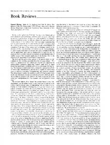
The median value of 2N+1 samples is given by x ~ + l ) , which for the example just given would be: n(?)=4. We thus have y k = 4. The window is then moved so it is centered over the k+l'st sample in the input sequence and the output value y k + 1 is computed by following the above procedure. Figure 1.1 shows the input and output for a window width three median filter, and also shows how the window moves along the signal. Note from the figure that the median filter can preserve edge structures while deleting impulsive structures.

5

I

:

I

I I

- 4 - 3 -2 -

Input

1

- 0 Wta Motion

2 4 53 & o 1

output

--

0 Fig. 1.1: The window width 3 (WW3) median filter. Several questions can now be asked. Since the median filter is nonlinear, what can we say about it when we can't use the traditional tools of linear analysis to understand it? Are there whole classes of filters with the median's ability to preserve details such as edges while removing noise?

CH 30064/91/oooO - OOO9 $1.00 0 IEEE

These questions have attracted the attention of a growing number of researchers over the last few decades. The result of this attention is a large number of papers, dissertations and books written on median and median-related filters. In the following subsections, we present a very brief literature review on this subject. The glaring omissions are order statistic filters, weighted median filters, vector median filters, selection filters, rank order processors, and =-filters. Other related areas not covered here are morphology, cellular automata and neural networks. For a full review, see [PiV] and [GCG].

With the above theoretical results, the success of median filters was becoming well understood and it was becoming clear which applications were well-suited for median filtering. For instance, its ability to preserve edges and delete impulsive structures combined with its robustness with respect to different noise types is why it has been used so extensively in image processing. AU of the above praise might lead one to believe that the median is the perfect filtering operation, which is not true. The median can introduce edge jitter and streaking into an image (see, for example, [BHMI). These shortcomings, and the desire to find other filters similar to the median but which allow more design choices than just the window width, has motivated many generalizations of the median filter (see [GCG][PiV] for a history).

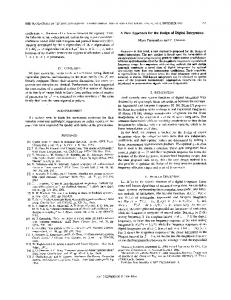
2. Theoretical Analysis of Median Filters In the 1970's, J.W. Tukey [Tuk, pg 2101 introduced the "running median" as a tool for smoothing discrete data. Since then, its name has changed to "median filter," and it has been used in several areas of digital signal processing, including speech processing, image enhancement, and seismic data analysis. Some of the earliest theoretical results on the behavior of the median filter concerned the existence and nature of its invariant signals, or root signals. An example of a root signal is provided in Figure 2.1, in which it is easy to see that the input and output signals are the same.

3. From Median Filters to Stack Filters In 1984, an important theoretical tool for analyzing median and median-type filters was developed by Fitch et al, [FCGl]. They showed [FCGl][FCG2] that all rank-order-based filters possess a weak superposition property called the threshold decomposition, which says that median filtering any sequence whose elements take on values in the set Q = [OJ, . . . M-1) is equivalent to decomposing the signal into binary sequences by thresholding at each level from 1 through M-I, filtering each resulting binary sequence by a (binary) median filter, and then adding up the results. TO express this property more precisely, define Ti(.) to be the operator which thresholds its argument at the level i:

For instance, T3(5)= 1 and T3(2)= 0. We will also apply thresholding to vectors, and wiU define it as follows: Ti(xJ,

. . * , Ti(x,,)](3.2)

For example, we would have T3[(6,2,1,3,7)] = (l,O,O,l,l). Then, suppose a median filter of window width 3 whose input sequence takes on values in Q . The threshold decomposition states that for every k

Fig. 2.1: Root signal of WW5 median filter. The locally monotone nature of these finite-length fixed points was proven for all median filters of odd window width in [Tyal and [GaWl. In [GaW] it was also shown that any finite length signal is filtered to a root signal after a finite number of passes of a median filter of a fixed window width. This is an important result -- it ties median-type filters to neural nets since such convergence behavior is the primary characteristic of associative memories. The many studies of the root signals and convergence behavior of the median filter form a significant part of what is now called the study of the structural behavior of median filters and median-type filters (see [CLG][GCG] for a review). The goal is to determine the type and number of root signals, whether every signal is filtered to a mot signal, and which structures are preserved, created, modified or deleted by median-type filters. The early studies of the structural behavior of the median filter complemented results known for quite some time in the statistics literature: the median of iid samples of a double exponential random variable is the maximum likelihood estimator of the mean of that random variable; and the conditional median at each time instant t is the minimum mean absolute e m r estimator of the signal value at time t , where the conditioning is on the past history up to time t of the noise corrupted observations of the signal.

Med(xk-lxkJk+l)

=Med

= Yi=lM e d k i [(Xk-lJk

Jk+l)l].

This weak superposition property, which is illustrated in the example provided in Figure 3.1, allows the analysis of the effects of the median on multi-valued sequences to be reduced to the study of its effects on binary sequences.

10

Stack frZters were defined as the class of digital filters having the threshold decomposition property and the ordering property [NaR], called the stacking property in [WCG], exhibited by the median filter. The stacking property led to a connection to positive Boolean functions [Gill. In Figure 3.2, we show the threshold decomposition architecture of a specific stack filter known as the asymmetric median filter. Mathematically, this figure states the following superposition property for the stack filter Sf(.) based on the positive Boolean function f (.): S f h - - l ~ k ~ k + 1= ) Sf

[""T:

Ti(h-lJkJk+l))

i=l

]

per time unit between the filter's output and the desired signal is minimized. If S 0')and R 0')are jointly stationary, then the cost to be minimized is

(