From Perception to Preference and on to Inference ... - Semantic Scholar

Psychological Review 2014, Vol. 121, No. 3, 501–525

© 2014 American Psychological Association 0033-295X/14/$12.00 http://dx.doi.org/10.1037/a0037025

From Perception to Preference and on to Inference: An Approach–Avoidance Analysis of Thresholds Shenghua Luan, Lael J. Schooler, and Gerd Gigerenzer

This document is copyrighted by the American Psychological Association or one of its allied publishers. This article is intended solely for the personal use of the individual user and is not to be disseminated broadly.

Max Planck Institute for Human Development, Berlin, Germany In a lexicographic semiorders model for preference, cues are searched in a subjective order, and an alternative is preferred if its value on a cue exceeds those of other alternatives by a threshold ⌬, akin to a just noticeable difference in perception. We generalized this model from preference to inference and refer to it as ⌬-inference. Unlike with preference, where accuracy is difficult to define, the problem a mind faces when making an inference is to select a ⌬ that can lead to accurate judgments. To find a solution to this problem, we applied Clyde Coombs’s theory of single-peaked preference functions. We show that the accuracy of ⌬-inference can be understood as an approach–avoidance conflict between the decreasing usefulness of the first cue and the increasing usefulness of subsequent cues as ⌬ grows larger, resulting in a single-peaked function between accuracy and ⌬. The peak of this function varies with the properties of the task environment: The more redundant the cues and the larger the differences in their information quality, the smaller the ⌬. An analysis of 39 real-world task environments led to the surprising result that the best inferences are made when ⌬ is 0, which implies relying almost exclusively on the best cue and ignoring the rest. This finding provides a new perspective on the take-the-best heuristic. Overall, our study demonstrates the potential of integrating and extending established concepts, models, and theories from perception and preference to improve our understanding of how the mind makes inferences. Keywords: simple heuristics, lexicographic semiorders, take-the-best, single-peaked function, ecological rationality Supplemental materials: http://dx.doi.org/10.1037/a0037025.supp

breakers, The New York Times based its ranking on the total number of medals. As detailed in an article from The Wall Street Journal (Johnson, 2008), both rules have their merits and advocates, resulting in this ranking controversy. The human mind faces a similar problem: how to infer which alternative is the best given conflicting cues. The rule used by the People’s Daily is a lexicographic rule that evaluates alternatives based on a set of cues ordered according to their importance. To compare the alternatives, the most important cue is checked first. If one alternative has an advantage over the others on this cue, it receives a higher ranking; if multiple alternatives have the same value on the cue, subsequent cues are checked. When alternatives share the same values on all cues, either a tie is declared or their rankings are determined randomly. This rule, which we refer to as the strict lexicographic rule, is a special case of a family of rules called lexicographic semiorders (Tversky, 1969), in which a threshold ⌬ is applied to determine if the difference between two alternatives on a cue is large enough to tell them apart meaningfully. In the strict lexicographic rule, ⌬ is set to zero. If ⌬ is set to 2 in the Olympics example (see the last column in Table 1), some rankings will change. For example, Australia is now ranked higher than Germany, because their difference in gold medals does not exceed two and Australia has five more silver medals. A lexicographic rule is noncompensatory in nature because higher values of the less important cues cannot compensate for lower values of the more important cues. In contrast, the rule adopted by The New York Times is compensatory because the three

During the 2008 Summer Olympic Games in Beijing, a heated contest took place alongside the individual competitions happening in the actual venues: the race between China and the United States to top the medal count. Table 1 shows the number of medals claimed by 10 countries in the games. Given these numbers, which country should be ranked number one? Because the International Olympic Committee refuses to publish its own final ranking, the task naturally falls to the individual countries and their respective news outlets. As seen in Table 1, The New York Times and the People’s Daily ranked their own countries first. The disparity is caused by the different rules the two newspapers adopted for ranking: Whereas the People’s Daily ranked countries according to gold medals, considering silver and bronze medals only as tie

Shenghua Luan, Lael J. Schooler, and Gerd Gigerenzer, Center for Adaptive Behavior and Cognition, Max Planck Institute for Human Development, Berlin, Germany. We thank Shuli Yu and Peng Huang for collecting 19 real-world environment data sets; Henry Brighton, Michael R. Dougherty, Konstantinos V. Katsikopoulos, Michael Lee, James Townsend, Peiqiu Zhao, and members of the ABC Research Group for their helpful comments; and Anita Todd and Rona Unrau for editing the manuscript. We are especially grateful to Tian Liu for her advice on statistical modeling and help in programming the simulations carried out for the real-world environments. Correspondence concerning this article should be addressed to Shenghua Luan, Lentzeallee 94, 14195 Berlin, Germany. E-mail: [email protected] 501

LUAN, SCHOOLER, AND GIGERENZER

502

Table 1 The Medal Counts and Rankings of 10 Countries in the 2008 Beijing Olympic Games


Ranking Country

Gold

Silver

Bronze

Total

Pointsa

The New York Times

Medal points

People’s Daily

LS, ⌬ ⫽ 2b

United States China Russia Britain Australia Germany France South Korea Italy Ukraine

36 51 23 19 14 16 7 13 8 7

38 21 21 13 15 10 16 10 10 5

36 28 28 15 17 15 17 8 10 15

110 100 72 47 46 41 40 31 28 27

330 346 206 149 132 125 100 103 80 65

1 2 3 4 5 6 7 8 9 10

2 1 3 4 5 6 8 7 9 11

2 1 3 4 6 5 10 7 9 11

2 1 3 4 5 6 8 7 9 10

a

Each country’s medal points were calculated following a rule used in the 1908 London Olympic Games: five for gold, three for silver, and one for bronze. b LS, ⌬ ⫽ 2 is lexicographic semiorders with ⌬ at 2.

medal types are treated as equally important; thus, a lower value of one can be fully compensated for by higher values of the others. This equal-weighting or tallying rule is a special case of a family of weighting-and-adding rules (Payne, Bettman, & Johnson, 1993), in which features or cues are weighted and their values added. An unequal-weighting rule can also be employed to rank countries. For instance, in the 1908 London Olympic Games, the following weighting scheme was used to calculate the overall medal points for a country: five for gold, three for silver, and one for bronze (Johnson, 2008). The points and rankings of the 10 countries according to this rule are shown in Table 1. Both lexicographic and weighting-and-adding rules were developed within the context of preference. Weighting-and-adding has always been the dominant view about the nature of preference, beginning in the mid-17th century with Blaise Pascal and Pierre Fermat’s expected value theory, which was then modified by Daniel Bernoulli to become expected utility theory (Daston, 1988). Today, the theory has branched into a host of descriptive models of preference (e.g., Busemeyer & Townsend, 1993; Kahneman & Tversky, 1979; Payne et al., 1993). The key alternative models to those derived from expected utility theory operate according to the lexicographic principle. According to Georgescu-Roegen (1968), the first to propose a lexicographic rule and ordering was Carl Menger, founder of the Austrian School of Economics. In his discussion of concrete needs such as air, food, and shelter for survival, Menger argued that the order should be lexicographic, meaning that the most fundamental needs must be taken care of first before turning to the less important ones. This view is present in motivational hierarchies (e.g., Maslow, 1954), as well as in moral theories that assume that not everything has a price (e.g., Gigerenzer, 2010). In studies of preference formation, a significant body of evidence has accumulated to support the use of lexicographic rules in practice (e.g., Bettman, Johnson, & Payne, 1990; Brandstätter, Gigerenzer, & Hertwig, 2006; Ford, Schmitt, Schechtman, Hults, & Doherty, 1989; Kohli & Jedidi, 2007; Lopes, 1995; Regenwetter, Dana, Davis-Stober, & Guo, 2011). In this study, we focused on the model of lexicographic semiorders and generalized it from preference to inference. Preference is a matter of taste, which can be evaluated by internal criteria such as consistency and transitivity. We use the term inference if an external criterion exists against which the accuracy of a judgment

can be assessed. For example, choosing what sports to watch in the Olympics is about preference, whereas predicting which country will win in a men’s basketball match is an inference. Various models based on both lexicographic and weighting-and-adding principles have been applied to inference tasks (e.g., Chater, Oaksford, Nakisa, & Redington, 2003; Gigerenzer & Brighton, 2009; Gigerenzer & Goldstein, 1996; Gigerenzer, Todd, & the ABC Research Group, 1999; Hogarth & Karelaia, 2007; Katsikopoulos, Schooler, & Hertwig, 2010). However, apart from one study that investigated how well lexicographic models with a threshold structure describe people’s inferences under time pressure (Rieskamp & Hoffrage, 2008), there has been no systematic analysis of such models’ performance with regard to the inferences they make. We addressed the following three questions in the present study: 1.

How can lexicographic semiorders be generalized from preference to inference? To answer this question, we defined the model in terms of three building blocks of fast and frugal heuristics (e.g., Gigerenzer & Goldstein, 1996; Gigerenzer et al., 1999), namely, the search, stopping, and decision rules.

2.

What is the general functional form of the relation between the quality of inference and the threshold ⌬? We derived the answer to this question using Clyde Coombs’s theory of single-peaked preference functions, which is rooted in Kurt Lewin’s conceptualization of approach–avoidance conflicts.

3.

How should a mind adapt ⌬ in response to the structure of the task environment? To address this question of ecological rationality—that is, when and why a certain ⌬ leads to sound inferences—we conducted two studies with simulated environments, followed by an analysis of real-world environments.

From Perception to Preference Concepts from psychophysics have facilitated theory development in decision making in many ways. For instance, framing absolute thresholds as aspiration levels, Herbert Simon (1956) formulated the satisficing heuristic, the prototype of his bounded-

APPROACH–AVOIDANCE ANALYSIS OF THRESHOLDS


rationality framework; Daniel Kahneman and Amos Tversky (1979) modeled the value functions in their prospect theory based on the power law between stimulus intensity and sensation; and signal detection theory, originally developed to advance perceptual thresholds beyond their deterministic nature (e.g., Gigerenzer & Murray, 1987; Tanner & Swets, 1954), has been used to model decision making of various kinds (e.g., Birnbaum, 1983; Haselton & Buss, 2000; Luan, Schooler, & Gigerenzer, 2011; Pleskac & Busemeyer, 2010; Wallsten & Gonzalez-Vallejo, 1994). Duncan Luce (1956) drew on the analogy between psychophysics and preference to challenge the notion in utility theory that indifference relations should be transitive: It is certainly well known from psychophysics that if “preference” is taken to mean which of two weights a person believes to be heavier after hefting them, and if “adjacent” weights are properly chosen, say a gram difference in a total weight of many grams, then a subject will be indifferent between any two “adjacent” weights. If indifference were transitive, then he would be unable to detect any weight differences, however great, which is patently false. (p. 179)

Assuming that the same general principles (e.g., Weber’s and Fechner’s laws) govern human discrimination of both weights and utilities, Luce proposed a theory of preference that incorporates just noticeable differences in the utility functions and allows for intransitive indifference relations. He defined semiorders as preference orders in which indifference relations result from small utility differences and that satisfy four simple axioms. Luce’s work on semiorders was seminal but did not strike at the core of utility theory because it still assumed that people form preferences by comparing the expected utilities of the alternatives. Applying the concept of semiorders to model the underlying decision process instead of the utility function, Tversky (1969) coined the term lexicographic semiorders to name a descriptive model in which “a semiorder or a just noticeable difference structure is imposed on a lexicographic ordering” (p. 32). Tversky provided several intuitive examples to explain how the model works and postulated that the selection of ⌬ would be subject to various individual and contextual factors, although he did not investigate these factors and their effects in his experiments. His main goal was to demonstrate intransitive choices by people who appear to decide using lexicographic semiorders (but see Birnbaum & Gutierrez, 2007, and Regenwetter, Dana, & Davis-Stober, 2011, who challenged Tversky’s experimental findings). In sum, combining semiorders (Luce, 1956)—a concept originating from just noticeable differences in perception—with the lexicographic procedure, Tversky (1969) formulated lexicographic semiorders as a descriptive model for preference; the model has since been found to describe a wide range of preferential choices (e.g., Bettman et al., 1990; Ford et al., 1989; Kohli & Jedidi, 2007; Lopes, 1995). In what follows, we describe how we extended this model from preference to inference.

From Preference to Inference To generalize lexicographic semiorders from preference to inference, we assume that the primary goal of the mind is to achieve a high level of accuracy. With this in mind, we specify a lexicographic model for paired-comparison inference tasks in which a person needs to infer which object of a pair has a larger criterion

503

value on the basis of relevant cues. The model has three building blocks: 1.

Search rule: Examine cues in the order of their accuracy, where accuracy is assessed for each cue independently from other cues.

2.

Stopping rule: If the difference between a pair of objects, A and B, on a cue exceeds a threshold value ⌬, then stop search.

3.

Decision rule: Infer that the object with the higher cue value is the one with the higher criterion value.1 If no difference exceeds ⌬ for all cues, then pick one object by guessing.

We refer to this model as ⌬-inference, acknowledging the key elements it inherits from lexicographic semiorders and emphasizing the central role ⌬ plays in the inference process. The search rule makes an explicit assumption about independence, which protects one from estimation errors by reducing variance at the cost of bias2 (e.g., Geman, Bienenstock, & Doursat, 1992). Models that make this simplifying independence assumption can outperform those that try to estimate dependencies, especially when sample size is small, the number of cues is large, and the environment is unstable (e.g., Gigerenzer & Brighton, 2009; Martignon & Hoffrage, 1999; Mussi, 2002). Similarly, the stopping rule assumes a uniform ⌬ across all cues after standardization instead of estimating a different ⌬ for each cue. The specific value of ⌬ in a task environment is either exogenously given or acquired from learning. For the decision rule, random guessing is used when no difference in any of the cues exceeds ⌬. In the General Discussion, we report the performance of two variants of ⌬-inference, one that allows ⌬ to vary for different cues and the other that tries to avoid guessing. Having defined ⌬-inference with three building blocks, we next address the question of how the accuracy of the model varies as a function of ⌬. Coombs’s theory of single-peaked preference functions (e.g., Coombs & Avrunin, 1977a) was instrumental in our attempt to answer this question. To explain how, we begin by describing our analysis of a task involving only two cues.

“Good Things Satiate, Bad Things Escalate” In a two-cue task environment, the accuracy of ⌬-inference in terms of percentage correct (PC) can be expressed as follows:

1 When lower cue values imply higher criterion values, cue values need to be reversed before applying the decision rule. 2 These two concepts are key to the bias–variance analysis in machine learning. In short, bias refers to how closely an algorithm mimics the true function that generated the observed data, and variance is how sensitive the accuracy of the algorithm is to different data samples. To obtain the best prediction accuracy, an algorithm would ideally be low in both bias and variance. However, there is often a tradeoff between the two, and algorithms with fewer parameters to estimate tend to have higher levels of bias but lower levels of variance relative to those with more parameters.


504

PC ⫽ DR1 ⫻ V1 ⫹ DR2 | 1 ⫻ V2 | 1 ⫹ GR ⫻ .5 ⫽ U1 ⫹ (U2 | 1 ⫹ UGuessing)

(1)


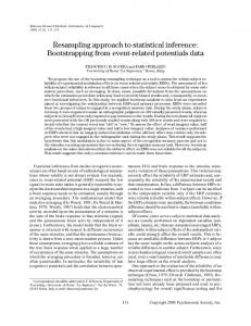
⫽ U1 ⫹ URest , where DR stands for decision rate, the probability that a cue leads to a decision3; V for validity, the probability that a decision made by the cue is correct; and GR for guessing rate, the probability that a decision is made through guessing. The subscript 2|1 highlights the conditional nature of the measures associated with the second cue: For example, V2|1 is the validity of the second cue given that the first cue fails to make a decision. In addition, the product of DR and V is the usefulness (U) of a cue, which represents the cue’s contribution to the overall accuracy of ⌬-inference. UGuessing is the usefulness from guessing and is simply the product of GR and the guessing accuracy of .5. Equation 1 shows that the accuracy of ⌬-inference is an additive function of the three usefulness components: U1, U2|1, and UGuessing. To further simplify the equation, we grouped the sum of the latter two components under the name URest. Understanding how the two usefulness measures, U1 and URest, change with ⌬ will facilitate our understanding of the effect of ⌬ on the accuracy of ⌬-inference. In general, we hypothesized that U1 would be a decreasing function of ⌬ and URest an increasing one based on the following rationale: As ⌬ becomes larger, more and more decisions will be made by the second cue or by guessing, increasing their contributions (i.e., URest) to the accuracy of ⌬-inference but reducing the contribution of the first cue (i.e., U1). We also hypothesized that the sum of U1 and URest would be a singlepeaked function of ⌬. This latter hypothesis is derived from previous research on the approach–avoidance conflict initiated by Lewin (e.g., Lewin, 1935, 1951; Lewin, Dembo, Festinger, & Sears, 1944) and the related work by Coombs on single-peaked preference functions (e.g., Coombs, 1964; Coombs & Avrunin, 1977a). The term approach–avoidance conflict was used by Lewin to depict a situation in which individuals are subjected to two opposing psychological forces, one pushing them toward a certain goal (approach) and the other pulling them away from it (avoidance). Lewin speculated that as a person moves closer to the goal, both forces would become stronger but that the force of avoidance would increase more steeply than that of approach. Empirical studies confirmed his speculation (e.g., Epstein & Fenz, 1965; Hunt, 1960; Miller, 1944, 1959), which was then summarized by Coombs and Avrunin (1977a) with a simple phrase: “Good things satiate, bad things escalate” (p. 224). Coombs and Avrunin argued that this principle of approach–avoidance conflict is applicable in many decision-making tasks and further showed that it is one crucial reason why preference is often a single-peaked function. Singlepeaked function implies the existence of an ideal point in an underlying scale, which is the cornerstone assumption of the unfolding theory for which Coombs is best known (Coombs, 1964). The left panel of Figure 1 shows how the principle works in an example introduced by Coombs and Avrunin (1977a). Suppose that you are taking a vacation for an indeterminate period of time t. The longer the vacation, the more you will be able to acquire new, exciting experiences or simply relax. In general, this positive utility, UGood, increases with t, and the function is

likely to be concave because, like many other goods, the accumulation of positive experience has a diminishing marginal return (good things satiate). However, not all is good during a vacation: The longer the stay, the more you will miss the comforts of home. Overall, this negative utility, UBad, is a decreasing function of t, and the function is likely to be concave too because the negative experience tends to become increasingly unpleasant toward the end (bad things escalate). As a result of these two functions, the total utility, UTotal, of the vacation becomes a single-peaked function of time. Coombs and Avrunin (1977a, 1977b) proved that as long as there is an approach–avoidance conflict in a nontrivial decision situation and the two forces follow the good things satiate, bad things escalate principle, preference will be a single-peaked function. Analogous to the above example, our hypothesized effects of ⌬ are visualized in the right panel of Figure 1. In the graph, U1, URest, and PC (i.e., the accuracy of ⌬-inference in percentage correct) correspond to UBad, UGood, and UTotal in the left panel, respectively, and the labels for the two axes, time and utility, are replaced by ⌬ and accuracy. If U1 decreases and URest increases monotonically as ⌬ becomes larger and if their functions follow the good things satiate, bad things escalate principle, then the accuracy of ⌬-inference should be a single-peaked function of ⌬.

A First Look Into ⌬-Inference With Simulated Environments To test the single-peaked function hypothesis, we conducted a study with three simulated two-cue environments. How the three building blocks of ⌬-inference were implemented in our tests of the model is summarized in Table 2. For the search rule, we ranked cues according to their ecological correlations (i.e., bivariate Pearson correlations) with the criterion because (a) following Egon Brunswik’s (1955) lens model, ecological correlation has long been used in judgment and decision-making studies as an indicator of cue quality (e.g., Brehmer & Joyce, 1988; Cooksey, 1996; Hammond & Stewart, 2001; Hogarth & Karelaia, 2007); (b) in paired-comparison inference tasks, it has been shown to be strongly related to the unconditional accuracy of a cue (e.g., Luan, Katsikopoulos, & Reimer, 2012; Rakow, Newell, Fayers, & Hersby, 2005); and (c) the rankings of cues’ ecological correlations are independent of the value of ⌬, thus separating the search rule from the stopping rule. For the stopping rule, ⌬ was measured in terms of a standardized z score; in this study, a range of ⌬ values, from 0 to 3.5 with a step size of 0.1, were applied. Each two-cue simulated environment consisted of three variables: one criterion Y and two cues, X1 and X2. Values of these

3 The decision rate (DR) of the first cue is the same as its discrimination rate (dr), the probability that two objects have different values on a cue when the cue is searched (e.g., Gigerenzer & Goldstein, 1996). For the second cue, however, the two diverge. Specifically, dr2|1 ⫽ DR2|1/(1 ⫺ DR1). What sets them apart is the reference class: For DR, the reference class is all pairs of objects within a sample, whereas, for dr, it is confined to pairs for which decisions cannot be made by previously searched cue or cues.



505

Figure 1. Single-peaked functions. The left panel shows how a single-peaked function can occur as a result of an approach–avoidance conflict in an example given by Coombs and Avrunin (1977a). The right panel shows our hypothesized effects of ⌬ on the two usefulness measures and the accuracy of ⌬-inference in percentage correct (PC) in a two-cue task environment.

variables were drawn from a multivariate normal distribution with means of 0 and the variance– covariance matrix

冢

1

␳1 ␳2

冣

M f(Y,X1,X2) ⫽ ␳1 1 r12 . ␳2 r12 1 In the matrix, ␳1 and ␳2 are the cues’ ecological correlations, and r12 is the correlation between the two cues; their values in the three environments are shown in Table 3. In Appendix A, we show how the cue measures that are relevant to our analysis can be expressed in probability terms and calculated mathematically for an arbitrary ⌬ in each environment.

Single-Peaked Function The effects of ⌬ on various cue measures and the accuracy of ⌬-inference (PC) in Environment A are shown in Figure 2. As seen in Figure 2A, with a larger ⌬, the validity of Cue 1 (V1) increases as its decision rate (DR1) decreases. Because the rate of improve-

ment for V1 is slower than the rate of deterioration for DR1, their product U1 is a monotonically decreasing function of ⌬, having its maximum at ⌬ ⫽ 0 and approaching zero when ⌬ grows very large. Figure 2B shows the effects of ⌬ on Cue 2’s validity (V2|1) and decision rate (DR2|1), as well as on the guessing rate (GR). Like V1, V2|1 also increases with ⌬; however, DR2|1 is now a single-peaked function of ⌬. This result can be understood in the following way: When ⌬ is very small, most decisions are made by Cue 1, leaving a low probability of Cue 2 being used; when ⌬ is very large, most decisions are made by guessing rather than by using any of the cues; therefore, the maximum probability of Cue 2 being used (DR2|1) must lie somewhere in between. The function of GR is simple: It increases monotonically as ⌬ grows larger. Effects of ⌬ on the usefulness of Cue 2 (U2|1) and guessing (UGuessing) and their sum URest are shown in Figure 2C. The functions of U2|1 and UGuessing track those of DR2|1 and GR (see Figure 2B), respectively, and the function of URest is apparently not affected much by that of U2|1 and is a monotonically increasing function of ⌬. Finally, Figure 2D shows the effect of ⌬ on the

Table 2 The Three Building Blocks of ⌬-Inference as Implemented in This Study Fine-tuning ⌬ Building block

Key question

Search

How are cues ordered?

Stopping

Does ⌬ take a uniform value across all cues after standardization? How is ⌬ set?

Decision

Is a decision made by guessing when the difference between two objects does not exceed ⌬ for any cue?

⌬-inference

Individual ⌬ for each cue

⌬-adjustment

Take-the-best

By ecological correlation Yes

By ecological correlation Not necessarily

By ecological correlation Yes

By validity

Exogenous or acquired from learning Yes

Exogenous or acquired from learning Yes

Exogenous or acquired from learning No; instead, repeat search from the first cue with a lower ⌬ value

Fixed at 0

Yes

Yes


506

Table 3 Values of the Key Parameters for the Three Simulated Two-Cue Environments


Parameter Environment

␳1

␳2

r12

A B C

.6 .6 .9

.5 .5 .2

.1 .7 .1

accuracy of ⌬-inference (PC), which is the sum of U1 and URest, together with the functions of U1 and URest. Here, an approach– avoidance conflict becomes clear: As ⌬ grows larger, URest increases, prompting one to approach an even larger ⌬, whereas U1 decreases, leading one to avoid adopting any ⌬ that is larger than

0. It is also clear that the functional forms of URest and U1 are in general consistent with the good things satiate, bad things escalate principle. As a result, the accuracy of ⌬-inference is a singlepeaked function of ⌬. In sum, the effects of ⌬ on U1, URest, and the accuracy of ⌬-inference in Environment A confirm our single-peaked hypothesis illustrated in the right panel of Figure 1. We also conducted the same analyses for Environments B and C (see their parameter values in Table 3), where the same pattern emerges—that is, the accuracy of ⌬-inference is a single-peaked function of ⌬ due to the conflict between U1 and URest. In Appendix B, we prove that U1 is a monotonically decreasing and URest a monotonically increasing function of ⌬ in any two-cue environment with the same distributional structure as the three environments discussed here, demonstrating the generality of this approach–avoidance conflict. According to Coombs and Avrunin (1977a, 1977b), in most cases,

Figure 2. The effects of ⌬ on various cue measures and the accuracy of ⌬-inference in a simulated two-cue environment. In this environment, the cues’ ecological correlations ␳1 and ␳2 and their intercue correlation r12 are .6, .5, and .1, respectively. V ⫽ validity; DR ⫽ decision rate; U ⫽ usefulness; GR ⫽ guessing rate; PC ⫽ the accuracy of ⌬-inference in percentage correct.



507

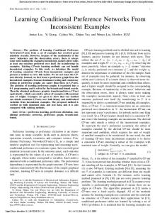
Figure 3. Finding Peak⌬, the ⌬ under which the accuracy of ⌬-inference peaks, in three simulated two-cue environments. The left panel shows the accuracy of ⌬-inference as a function of ⌬, with Peak⌬ indicated by a rectangular box, in each environment; the right panel shows the change in URest minus the change in U1 (⳵URest ⫺ ⳵U1) as a function of the change in ⌬ in each environment. According to the change inequality, one should stop adopting a larger ⌬ when (⳵URest ⫺ ⳵U1) ⬎ 0. A dashed line is added in the right panel to indicate the point at which this occurs for each environment. U ⫽ usefulness.

the conflict by itself is sufficient to induce a single-peaked preference function.

Effects of Environmental Properties on the Selection of ⌬ Despite the existence of a single-peaked function in each of the three environments, they do differ in the value of ⌬ under which the peak of the function is reached. The accuracy of ⌬-inference as a function of ⌬ in each two-cue environment is shown in the left panel of Figure 3. In the figure, the ⌬ under which the function peaks, which we refer to as Peak⌬, is seen to be 0.6 (in z score) in Environment A but much smaller in B and C, where it is 0.2 and 0.1, respectively. Because Environments A and B differ in r12 (.1 vs. .7), the intercue correlation that is often taken as a measure of information redundancy (Hogarth & Karelaia, 2007), this environmental property appears to be negatively related to Peak⌬. Environments A and C, on the other hand, differ in the value of ␳1 ⫺ ␳2 (.1 vs. .7), the disparity between the two cues’ ecological correlations, which seems to be negatively related to Peak⌬ as well. Larger values of r12 imply that the second cue is more likely to contain information that is redundant to the information in the first cue, and larger values in ␳1 ⫺ ␳2 indicate that the second cue lags further behind the first cue in quality. In both cases, the second cue has less to offer, making the adoption of a large ⌬ unnecessary. However, it is not clear from the left panel of Figure 3 why Peak⌬ takes the specific values that it does in each environment. We explain in the following how these values come about. Suppose that one needs to decide whether to increase ⌬ from a smaller value ⌬j to a larger value ⌬k and is concerned solely with the effect of such a change on the accuracy of ⌬-inference (PC). In this case, one should make the change if and only if

PC(⌬k) ⫺ PC(⌬ j) ⬎ 0. On the basis of Equation 1, this inequality can be expanded to [U1(⌬k) ⫹ URest(⌬k)] ⫺ [U1(⌬ j) ⫹ URest(⌬ j)] ⬎ 0 ⫽ ⬎ [URest(⌬k) ⫺ URest(⌬ j)] ⬎ [U1(⌬ j) ⫺ U1(⌬k)]. Because the left-hand side represents the change in URest (⳵URest) and the right-hand side the change in U1 (⳵U1), the inequality is equivalent to ⭸URest ⬎ ⭸U1 or (⭸URest⫺ ⭸U1) ⬎ 0. We call this resulting inequality the change inequality. It implies that one should continue seeking a larger ⌬ as long as the change in URest remains larger than that of U1 and stop doing so when it is not. In other words, the highest level of accuracy will be reached when the growth of URest cannot catch the deterioration of U1, leading to a net reduction in accuracy. If the functional forms of ⳵URest and ⳵U1 are known and not overly complicated, then it is possible to derive mathematically the exact ⌬ above which the inequality fails to hold, and that ⌬ will be the Peak⌬ in an environment. However, the functional forms of ⳵URest and ⳵U1, especially the former, are indeed quite complicated (see Appendix B). Therefore, we obtained the critical ⌬ value in each environment numerically. The results are shown in the right panel of Figure 3. In the figure, the x-axis is the change in 0.1 z score between two ⌬ values (i.e., ⌬k ⫽ ⌬j ⫹ 0.1), and the y-axis is ⳵URest ⫺ ⳵U1, the change in URest minus the change in U1. As the figure shows, ⳵URest ⫺ ⳵U1 starts to become negative when ⌬ changes from 0.6 to 0.7, 0.2 to 0.3, and 0.1 to 0.2 in Environments A, B, and C, respectively. These transitions imply that the corresponding Peak⌬ should be 0.6, 0.2, and 0.1 in each of the environments, consistent with the results displayed in the left panel of Figure 3.


508

Knowing how the accuracy of ⌬-inference varies with ⌬ in an environment offers a direct way to locate the Peak⌬ in the environment. The change inequality and the ensuing analysis, on the other hand, make it easier to understand the dynamics behind the function and why Peak⌬ takes a certain value in a particular environment. Our analysis shows that when either r12 or ␳1 ⫺ ␳2 is relatively high in an environment, the gain of URest will increase at a slower pace than will the loss of U1 as ⌬ moves away from zero; as a result, the difference in their rates (⳵URest ⫺ ⳵U1) will quickly become negative, leading to a small Peak⌬ value.


Summary In this study, we first explored the effect of ⌬ on the accuracy of ⌬-inference. Drawing upon previous research on approach– avoidance conflicts and single-peaked preference functions, we hypothesized that the accuracy of ⌬-inference would be a singlepeaked function of ⌬; results from 3 two-cue environments confirm this hypothesis. Defining Peak⌬ as the ⌬ that leads to the highest accuracy of ⌬-inference in an environment, we then investigated how Peak⌬ is related to two environmental properties. The change inequality shows that Peak⌬ is determined by the difference in two rates—the increase in the usefulness of Cue 2 and guessing as well as the decrease in the usefulness of Cue 1 as ⌬ gets larger—and that Peak⌬ is the ⌬ above which this difference starts turning negative. We found that this transition point tends to occur earlier when the information redundancy between the cues is higher or the disparity between the cues’ ecological correlations larger. These results give us a preliminary understanding of ⌬-inference’s performance. However, because they were derived from three environments with a very simple information structure, it was necessary to check the generalizability of the results.

Table 4 The Number of Environments in Each Dispersion ⫻ Redundancy Category for the Simulated Three-Cue and Real Environments Simulated environments Dispersion

r ⱕ .4

r ⬎ .4

r៮ ⬍ .4

r៮ ⬎ .4

Equal Compensatory Noncompensatory

31 258 256

42 155 4

0 8 5

7 15 4

a

In each real environment, only the three cues with the highest ecological correlations were considered to identify its dispersion and redundancy. Moreover, the following rule was used to define an equal environment there: |␳1| ⫺ |␳3| ⱕ .10.

matical constraints,4 a total of 746 environments can be constructed; all were included here. Each environment was further characterized by the following three properties: 1.

Redundancy. This property is measured by the uniform intercue correlation r. To simplify the classification of the environments, we divide this property into two categories: low, if r ⱕ .4; and high, if r ⬎ .4.

2.

Dispersion. This property can have three values: equal, if all cues’ ecological correlations are equal, that is, if ␳1 ⫽ ␳2 ⫽ ␳3; compensatory, if ␳1 ⬍ (␳2 ⫹ ␳3); and noncompensatory, if ␳1 ⱖ (␳2 ⫹ ␳3). Dispersion provides a rough measure of the importance of Cue 1 relative to that of the other two cues (Hogarth & Karelaia, 2007). Note that compensatory and noncompensatory are used here to characterize task environments and should be distinguished from their usage in describing the nature of decision strategies.

3.

Linear predictability. This property is the total amount of variance in criterion Y that can be accounted for by the best fitting regression using the three cues as predictors (i.e., the R2 value of the regression). In lens-model analyses (e.g., Cooksey, 1996), this measure is often taken as an estimate for the total amount of information contained in an environment.

A Systematic Analysis of ⌬-Inference With Simulated Environments In this study, we examined if results from the previous study could be replicated by constructing a broad range of simulated environments, each characterized by a unique combination of ecological correlations and intercue correlations. More importantly, we also investigated the fitting and out-of-sample prediction accuracy of ⌬-inference in samples of various sizes, tested under what conditions one would be better off learning the Peak⌬ for each environment as opposed to using a fixed ⌬ across all environments, and compared ⌬-inference’s performance with that of a benchmark model (linear regression). In our subsequent study of the real-world environments, these kinds of analyses revealed a result about ⌬ that we never expected.

Environment Construction and Properties The environments in this study are similar to those simulated in the previous study but with three instead of two cues. In each environment, the value of an ecological correlation ␳i was positive and specified to one decimal place. For example, ␳is could be [.8, .4, .2], but not [.8, .4, ⫺.2] or [.81, .39, .18]. In addition, all intercue correlations were set to be equal in an environment, and this uniform correlation r was varied from 0 to .9 with a step size of .1. Following these specifications and with additional mathe-

Real environmentsa

The number of environments in each Dispersion ⫻ Redundancy category is shown in Table 4.

Fitting and Prediction Accuracy In each environment, we drew random samples of three sizes, N ⫽ 20, 100, and 2,000, and derived both the fitting and prediction accuracy of ⌬-inference. For each sample, we split it randomly into even halves to create a training set and a generalization set. In 4 For example, it is impossible to construct an environment with ␳is ⫽ [.9, .8, .1] and r ⫽ .8. The high intercue correlation excludes the possibility that one cue can have a much lower or higher ecological correlation than the others. Details of each simulated environment included in this study can be found in the online supplemental materials.



509

Figure 4. The Peak⌬, averaged over all simulated three-cue or real environments, in each Dispersion ⫻ Redundancy environment category. The left panel shows results from the simulated three-cue environments when sample size is 2,000, and the right panel shows results from the real environments when the size of the training set is 50% of a sample. Note that no real environments fall into the equal, low redundancy category.

the training set, we estimated the parameters needed to implement ⌬-inference and obtained the model’s fitting accuracy; in the generalization set, we applied the estimated parameters to derive the model’s prediction accuracy. To implement the search rule of ⌬-inference, the ecological correlations of the cues (␳is) need to be ranked, and for its stopping rule, a ⌬ needs to be set. If ⌬ is fixed at a certain value, then only the ranks of ␳is need to be estimated. However, if ⌬ is needed to achieve a certain goal (e.g., maximizing accuracy), it too needs to be estimated. We varied ⌬ from a z score of 0 to 1.5 with a step size of 0.1. In each sample, we derived the fitting and prediction accuracy of ⌬-inference under each ⌬ value. In addition, we also compared the fitting accuracy from all ⌬ values in the training set, identified Peak⌬ as the ⌬ value that led to the highest fitting accuracy, and examined the prediction accuracy of ⌬-inference with Peak⌬ in the generalization set.

Summary of Results The main results of this study are summarized below. Does the single-peaked function hold generally? The answer is yes. We found that in each and every condition (i.e., for both fitting and prediction accuracy, in each of the 746 environments, and with all three sample sizes), U1 is a monotonically decreasing function and URest (now equal to U2|1 ⫹ U3|1,2 ⫹ UGuessing) a monotonically increasing function of ⌬; as a consequence, the accuracy of ⌬-inference is a single-peaked function of ⌬. What properties of the environment influence Peak⌬? Consistent with the two-cue study, on average, the higher the redundancy among the cues and the higher the dispersion (i.e., the more an environment tends to be noncompensatory), the smaller the Peak⌬ (see Figure 4). In contrast, linear predictability has only a negligible effect on Peak⌬.5 This result helps us understand one

important aspect of the ecological rationality of ⌬-inference, that is, the match between the size of ⌬ and environmental structures.6 Small ⌬s are ecologically rational when cues are highly redundant and/or the best cue is of substantially higher quality than the other cues, irrespective of the environment’s linear predictability. When should one try to estimate Peak⌬ in each individual environment instead of using a fixed ⌬ across all environments? Averaged across 746 environments, the accuracy of ⌬-inference is a single-peaked function of ⌬; for prediction, it peaks at 0.5 z score in each sample-size condition (see Figure 5). Using a fixed ⌬ of 0.5 across all environments on average leads to slightly worse prediction accuracy— by half a percentage point—than using Peak⌬ for each environment when sample size is 2,000 (see the left panel of Figure 6). However, it 5 In the sample size ⫽ 2,000 condition, the correlation between the linear predictability of an environment and the value of Peak⌬ is ⫺.07. However, linear predictability is highly correlated with the prediction accuracy of ⌬-inference using Peak⌬: The correlation between the two is .98, whereas the correlations between the prediction accuracy and the two other properties, redundancy and dispersion, are ⫺.02 and .21, respectively. The same pattern of results is observed for the other two sample sizes. 6 Central to the study of ecological rationality is the investigation of how environmental structures influence the selection of mental strategies (e.g., lexicographic vs. weighting-and-adding) and, within a certain strategy, the selection of its key parameter values, such as the exit structure of a fast-and-frugal tree (e.g., Luan et al., 2011) and the weighting scheme of a linear model (e.g., Hogarth & Karelaia, 2007). If strategy selection is analogous to picking a proper tool (e.g., a wrench) from a toolbox for a certain type of task (e.g., Gigerenzer & Selten, 2002), then parameter selection can be thought of as further adjustments of the tool (e.g., on the jaws of a wrench) to make it more suitable for the specific task at hand (e.g., Lee & Cummins, 2004; Newell, 2005; Newell, Collins, & Lee, 2007). A complementary understanding of how both strategies and their key parameters are selected is essential for explaining how the mind adapts to different task environments.


510


Figure 5. The fitting and prediction accuracy of ⌬-inference, averaged over 746 simulated three-cue environments, under a set of fixed ⌬ values in three sample sizes: N ⫽ 20, 100, and 2,000. For each sample-size condition, i random samples were run, with i selected such that a total of 200,000 objects were simulated in each condition (e.g., i ⫽ 2,000 for N ⫽ 100). PC ⫽ percentage correct.

results in better prediction accuracy— by 0.8 percentage points— when sample size is 20 (see Table 5). The strong tendency for ⌬-inference with Peak⌬ to overfit the data when sample sizes are small is the main reason for this result.

How does ⌬-inference compare to linear regression? Because we constructed the simulated environments in a way that ideally suits linear regression, its accuracy should constitute an upper benchmark for performance. As expected, when sample size is 2,000, ⌬-inference with Peak⌬, which has better prediction accuracy than ⌬-inference with ⌬ ⫽ 0.5, is less accurate than linear regression by over two percentage points in prediction (see Table 5). However, when sample size is 20, ⌬-inference with ⌬ ⫽ 0.5, which now has better prediction accuracy than ⌬-inference with Peak⌬, is only a tenth of a percentage point less accurate in prediction than linear regression. It even outperforms linear regression in 104 (14%) and 424 (57%) environments when sample size is 100 and 20, respectively. These results were derived from simulated environments in which key environmental parameters and properties were systematically varied and comprehensively covered. This enables us to understand how ⌬-inference performs in theory and how its performance should be related to these environmental properties. However, there are two inherent limitations of our simulated environments: (a) They may be too idealized to represent environments in the real world, due to the relatively small number of cues in a task, the normally distributed cue values, and the constraints on cues’ ecological correlations and the intercue correlations; and (b) the parameters were sampled uniformly to increase the scope of their values but without regard to how they are distributed in the real world. These limitations raise yet another question of generalizability: How do the results from simulated environments hold up in realworld environments in which inference tasks actually take place?

Figure 6. The accuracy of ⌬-inference, averaged over all simulated three-cue or real environments, under different fixed ⌬ values. The left panel shows results from the simulated environments when sample size is 2,000, and the right panel shows results from the real environments when the size of the training set is 50% of a sample. In each panel, a dashed line indicates the average prediction accuracy of ⌬-inference with Peak⌬ for each environment. PC ⫽ percentage correct.


511

Table 5 The Average Accuracy (in Percentage Correct) of Three Models in the Simulated Three-Cue Environments


Fitting

Prediction

Model

N ⫽ 20

N ⫽ 100

N ⫽ 2,000

N ⫽ 20

N ⫽ 100

N ⫽ 2,000

Linear regression ⌬-inference with Peak⌬ ⌬-inference with ⌬ ⫽ 0.5

82.0 82.0 76.9

78.3 76.5 75.4

77.6 75.4 74.9

73.5 72.6 73.4

76.8 74.6 74.5

77.5 75.3 74.8

A Reality Check of ⌬-Inference in Real-World Environments In this study, we collected 39 real-world data sets from various sources (see Appendix C for a summary of the data sets). Given that these real-world environments differ from the simulated environments in many aspects, our main interest was to find out if those incongruities would alter our previous conclusions regarding the performance of ⌬-inference.

Properties of the Real-World Environments The 39 real-world data sets cover topics from a variety of fields, such as psychology, sociology, biology, consumer behavior, economics, and engineering. In each data set, there is one criterion variable and several cues related to it. For example, in the data set diamond price, the criterion is the price of a diamond, and the four cues are carat, clarity, color, and cut, which are commonly known as the four Cs. The number of cues in each data set varies substantially, ranging from two to 18 (M ⫽ 7.0, SD ⫽ 4.1). The majority of these cues are nonbinary (89%). Indeed, in 25 of the 39 data sets, there is not a single binary cue; in the rest, the majority of the cues are not binary, except for the German city population data set in which all cues are binary. With regard to the ecological correlations of the cues, the values for many are negative. Without altering their diagnosticities, we recoded all negative correlations as positive. In general, the best cues are quite good, with an average ecological correlation of .77 (SD ⫽ .15), and the second and third best cues are not bad either, with average ecological correlations of .60 (SD ⫽ .19) and .44 (SD ⫽ .24), respectively. Focusing strictly on the three best cues, we defined redundancy in a real environment as the average intercue correlation among these cues ( r៮). Averaged over all environments, the mean r៮ is .55 (SD ⫽ .26). Using the cutoff of .4, we further classified each environment as either highly redundant or less so. As a result, 67% (26/39) of the real environments were characterized as highly redundant, a substantially higher proportion than in the simulated environments (27%; see Table 4). High redundancy indicates that the information contained in cues searched after the first one is less useful, making these cues more dispensable. Figure 7 shows such effects in the simulated and real environments. Each panel displays the average correlations of the top three cues with the criterion. Shown are both the cues’ bivariate correlations, which define their ecological correlations, and their partial correlations after controlling for cues with higher bivariate correlations than theirs. Partial correlations, if estimated with sufficient accuracy, are more indicative of cues’ contributions to the performance of a model than bivariate correlations, especially for models employing sequential search. It is clear from the figure that the partial correlations of Cues 2 and 3 are lower than their bivariate correlations and that the differences are much larger in the real environments than in the simulated environments. Thus, due to higher cue

redundancy, the potential contributions of the second and third best cues are reduced to a greater extent in the real environments, enhancing the relative importance of the best cue. Recall that we use dispersion to characterize the importance of the best cue relative to the others and that the three levels of dispersion are defined based on the relations among cues’ ecological (or bivariate) correlations. Again focusing on the top three cues, Table 4 shows that only nine real environments (23%) are noncompensatory, a lower proportion than of the simulated environments (35%). However, if we revise the definition of dispersion from bivariate correlations to partial correlations (of cues after the best one), Figure 7 shows that collectively, the real environments become noncompensatory—that is, ␳1 ⱖ (␳2 ⫹ ␳3)—while the simulated environments remain compensatory. In sum, the 39 real-world environments included in our investigation are quite diverse, as shown by the wide ranges of values on relevant environmental parameters. Compared with an average simulated environment, in an average real environment, there tend to be more cues that a model can potentially use, a higher level of redundancy among the three cues with the highest ecological correlations, and a best cue that is relatively more important than the other cues. How such characteristics of the real environments affect the performance of an inference model, particularly ⌬-inference, is considered next.

Model Testing Our tests of models’ performance in the real environments differed from those in the simulated environments in four ways: First, in ⌬-inference, the threshold ⌬ was defined as a percentage of a cue value range instead of a z score. For instance, if the minimum and maximum values of a cue in a sample are 5 and 205, the cue has a range of 200, and then, a ⌬ of 5% will be 10. We used this definition of ⌬ because cue values can rarely be described by well-defined distributions and there are many noncontinuous cues in the real environments.7 Second, we varied the size of the training set, in terms 7 Although ⌬ is defined with different units in the simulated and real environments, the two can actually be compared directly. Specifically, in the simulated environments, one can estimate the range of cue values in a sample and then convert a percentage of this range to a z score. For example, based on 10,000 random samples with sample size N ⫽ 100, we estimated that cue values on average range from ⫺2.51 to 2.51 z scores in a sample, giving the whole range a 5.02 z score. Therefore, 1%, 5%, and 10% of this range result in a z score of 0.05, 0.25, and 0.50, respectively. We have now learned that setting ⌬ to 0.50 z score leads on average to the best prediction accuracy of ⌬-inference with a fixed ⌬ in the simulated environments. In terms of cue range percentage, that is equal to a ⌬ of 10% when sample size is 100. When sample sizes are 20 and 2,000, the percentages are about 14% and 7%, respectively.



512

Figure 7. Average correlations of the top three cues with the criterion variable in the simulated three-cue and real environments. The solid lines indicate cues’ bivariate correlations with the criterion, and the dashed lines indicate their partial correlations with the criterion after controlling for the cue or cues with higher bivariate correlation(s).

of a percentage of the entire sample, in each environment. The performance of a model was obtained by averaging the results from 500 random splits in each training-set condition. Third, in addition to linear regression, three other models were tested and compared to ⌬-inference. And finally, we examined how the performance of ⌬-inference depends on the specific criterion used to order cues by testing four alternatives to ecological correlation.

Zero Is the Best Fixed ⌬ in the Real-World Environments We started our investigation by setting the training set at 50% of a sample. Following the analysis procedures in the simulated environments, we first checked if the accuracy of ⌬-inference is a single-peaked function of ⌬ in the real environments. In 35 of the 39 environments, it is a single-peaked function for both fitting and prediction accuracy; in the remaining four, the functions are close to being single peaked. This result supports the generality of the single-peaked function beyond controlled environments. We next examined how Peak⌬ is related to environmental properties; the average Peak⌬ in each Dispersion ⫻ Redundancy category is shown in the right panel of Figure 4. The results are similar to those from the simulated environments: The higher the redundancy of the cues and the more an environment tends to be noncompensatory, the smaller the Peak⌬. We found the Peak⌬ in each environment by comparing the fitting accuracy of ⌬-inference under 51 ⌬ values, from 0% to 50% of a cue value range with a step size of 1%, and identifying the one that led to the highest accuracy as Peak⌬. The right panel of Figure 6 shows the fitting and prediction accuracy, averaged over all environments, of ⌬-inference under each ⌬. It is evident that the single-peaked function holds at the aggregate level in the real environments. However, instead of reaching its peak at a small but nonzero ⌬, the peak is now at zero for both fitting and prediction. In other words, among all the 51 fixed ⌬ values, zero is the best in the real environments!

⌬-inference with ⌬ ⫽ 0 is structurally equivalent to the strict lexicographic rule in preference and has a set of special properties. First, setting ⌬ at 0 means that a decision is made as soon as there is any difference in cue values between a pair of objects. In tasks where each object has a unique value on the first cue, that cue alone can be used to make all the decisions. Second, even if objects sometimes have identical values on the first or other cues, this model will still search, on average, the fewest number of cues in comparison to ⌬-inference with other ⌬ values. And third, in terms of mental operations (e.g., Bettman et al., 1990), it should be the simplest. With ⌬ at 0, it is not necessary for a person to compute exactly how objects differ on a cue to determine if the difference exceeds the threshold. All that is needed is a directional estimate: Does A have a higher value than B? With these attractive properties, how does ⌬-inference with a fixed ⌬ of 0 across all environments compare to ⌬-inference with Peak⌬ for each environment? The horizontal line in the right panel of Figure 6 shows the average prediction accuracy of ⌬-inference with Peak⌬. It is higher than that of ⌬-inference with ⌬ ⫽ 0 by about one 40th of a percentage point and is actually worse than ⌬-inference with ⌬ ⫽ 0 in the majority of the environments (22/39, or 56%). In terms of frugality, ⌬-inference with Peak⌬ searches, on average, 1.71 cues (SD ⫽ 0.71) in the generalization set, fewer than a quarter of all cues available (M ⫽ 7.0). Meanwhile, ⌬-inference with ⌬ ⫽ 0 searches only 1.14 cues (SD ⫽ 0.52), indicating that it rarely searches beyond the first cue. Being extremely frugal in search and simple to implement, ⌬-inference with ⌬ ⫽ 0 is also better than or as good as other ⌬-inference models in prediction accuracy. Why? The main reason is the enhanced relative importance of the best cues in the real environments. The selection of a proper ⌬ value depends heavily on how much additional information the cues following the first one can bring. If their contribution is substantial, ⌬ should be large, so that more decisions can be made by those cues; otherwise, ⌬ should be small. Our analysis shows that the information con-



Figure 8. The average fitting and prediction accuracy of three inference models in the real environments, when the size of the training set is 50% of a sample. PC ⫽ percentage correct.

tained in the cues after the best one is indeed very limited in the real environments (see Figure 7), justifying the selection of a small ⌬ value. What was unexpected for us, however, is that the best ⌬ turns out to be zero, the smallest possible. Further analyses show that avoiding the use of cues whose directions for inference may be improperly estimated can be a critical reason why zero stands out as the best. Specifically, in ⌬-inference, cues are ranked according to their bivariate correlations with the criterion and are used according to the directions of such correlations. With sufficient data, however, one will be better off basing inferences on the directions of cues’ partial correlations, which may be at odds with those of bivariate correlations. Indeed, correlation signs flip for 25 of the 77 second and third best cues in the real environments (33%). Such discrepancies will result in more misguided inferences when these cues are used and reduce the overall accuracy of ⌬-inference.8 With ⌬ at 0, however, this estimation problem is largely avoided because cues beyond the first one are rarely searched. Finally, we examined how the two ⌬-inference models, with Peak⌬ and with ⌬ ⫽ 0, fare against linear regression; the results are shown in Figure 8. For fitting, linear regression tops ⌬-inference with Peak⌬, which outperforms ⌬-inference with ⌬ ⫽ 0, and their differences are substantial. However, a different order emerges for prediction: ⌬-inference with Peak⌬ beats ⌬-inference with ⌬ ⫽ 0, which tops linear regression, although the differences among the three are quite small. If fitting is regarded as the means and prediction as the end in the pursuit of accurate inferences, these results show that all three models reach similar ends eventually, only taking different routes to get there. Among them, linear regression likely takes the most difficult route and ⌬-inference with ⌬ ⫽ 0 the easiest because the former must consider all the cues and their interactions in learning whereas the latter needs to learn only the order of cues’ ecological correlations.

Extended Model Testing and Comparisons To get a more comprehensive understanding of ⌬-inference’s performance, we extended model testing and comparisons in the

513

real environments in two ways: adding two more training-set conditions and comparing ⌬-inference with three new models, take-the-best, Bayesian linear regression, and the general monotone model (GeMM; Dougherty & Thomas, 2012). The details of these models and how they were implemented in our study can be found in Appendix D. While testing GeMM, we found that the minimal training set needed for the model differs across the 39 environments. Specifically, it is less than or equal to 20% of a sample for 12 environments, between 30% and 50% for 13 environments, and larger than 50% for the remaining 14 environments. In one of the two new training-set conditions, we set the training set in each environment in accordance with the minimal training set for GeMM and refer to it as minimal for GeMM. In the other condition, the training set is 80% of a sample. Unlike in the 50% condition in which the training set is not large enough for GeMM to produce reliable parameter estimates in all 39 environments,9 there is no such problem in the 80% condition. The average prediction accuracy of each model is displayed in Figure 9. It shows that first, take-the-best with dichotomized cues performs well below the other models (see more on this result in the General Discussion); second, regular linear regression dominates Bayesian linear regression, although their performance difference appears to get smaller with a larger training set; and third, GeMM performs quite well in the two conditions in which it can be directly compared to the other models. Regarding ⌬-inference, it can be seen that ⌬-inference with ⌬ ⫽ 0 performs best when training sets are smaller but falls short of the competition as the training set becomes larger (80%). This is consistent with results from other modelcomparison studies: With a larger training set, flexible models with more free parameters, such as linear regression and GeMM, can estimate parameters that capture the interactions among the cues more accurately, thus improving their prediction accuracy more. We also found that the prediction accuracy of ⌬-inference is a single-peaked function of ⌬ at the aggregate level in the two new training-set conditions. The best fixed ⌬ remains zero in the 80% condition but becomes 1% of the cue value range in the minimal for GeMM condition. Finally, we noticed that while the frugality of ⌬-inference with ⌬ ⫽ 0 remains rather constant in all training-set conditions, ⌬-inference with Peak⌬ tends to search fewer cues when the training set becomes larger, due to the generally lower Peak⌬ 8 The same problem also exists in the simulated environments, but to a much lesser degree. Among the 1,492 second and third best cues in the 746 environments, signs of 238 (16%) flip between the bivariate and partial correlations. 9 When the training set is 50% of a sample, GeMM cannot produce reliable parameter estimates in 14 environments. However, this occurs only for the version of GeMM that uses the Bayesian information criterion (BIC) for model selection (see Appendix D). Without this model-selection constraint, GeMM is able to produce reliable parameter estimates in all 39 environments. However, when the training set is smaller than 50% of a sample, even this version of GeMM does not work in some of the environments because the number of cues sometimes exceeds the number of cases. Results of GeMM without BIC model selection in the 50% and 80% training-set conditions can be found in the online supplemental materials.



514

Figure 9. The average prediction accuracy of six inference models in the real environments. Minimal for GeMM means that the training set is set at a minimal percentage of a sample (starting at 10%) so that reliable parameter estimates can be obtained for the general monotone model (GeMM) in each environment. There is no report of GeMM’s performance in the training set ⫽ 50% condition because the training set is not large enough to generate reliable parameter estimates in 14 of the 39 environments. Take-the-best was originally developed for tasks with binary cues. In this study, nonbinary cues were first dichotomized at the median before being processed by take-the-best. PC ⫽ percentage correct.

values in such conditions. Details of ⌬-inference’s performance can be found in the online supplemental materials.

⌬-Inference With Different Cue-Ordering Criteria In the definition of ⌬-inference, the search rule states that cues are ordered by accuracy. In our investigations so far, we have ordered cues by their ecological correlations. Does this specific choice matter? There are plenty of theoretical and empirical accounts of how people order cues; we tested four of these here (see

Table 6). Among the four, maximizing Kendall’s tau is the goal of GeMM (Dougherty & Thomas, 2012); Goodman–Kruskal’s gamma is a linear transformation of cue validity, the cue-ordering criterion in take-the-best (Martignon & Hoffrage, 2002); success will lead to the same cue order as ranking cues by their expected information gains (e.g., Newell, Rakow, Weston, & Shanks, 2004; Rakow, Hinvest, Jackson, & Palmer, 2004; Rakow et al., 2005); and usefulness, the cue measure that appeared in our discussion of the single-peaked function (see Equation 1), has also been studied as a cue-ordering criterion for take-the-best (e.g., Gigerenzer, Dieckmann, & Gaissmaier, 2012). It can be shown that in the absence of ties, these four measures will result in the same cue ordering; thus, ordering cues simply by counting the numbers of correct decisions they make (i.e., usefulness) is sufficient in this case. We found that for each of the alternative cue-ordering criteria and in each training-set condition, (a) the single-peaked function between ⌬-inference’s prediction accuracy and ⌬ holds at the aggregate level, and (b) zero is, on average, the best fixed ⌬ across all the real environments. Thus, specific cue-ordering criteria appear to have little effect on these two characteristics of ⌬-inference’s performance in the real environments. (A fuller account of these results can be found in the online supplemental materials.) Furthermore, ordering cues by success and usefulness lead to substantially worse prediction accuracy—typically by more than three percentage points—than tau, gamma, and ecological correlation (see Figure 10). The latter three perform at similar levels, with a slight advantage for tau. This result implies that tau could be a better cue-ordering criterion than ecological correlation and warrants further investigation. As mentioned earlier, ordering cues according to ecological correlation produces orders that do not depend on the value of ⌬. In the comparisons shown in Figure 10, we calculated tau, gamma, success, and usefulness of a cue by setting ⌬ to zero. Other ⌬ values will result in more cases in which a cue fails to make decisions and can alter values of these measures. Our preliminary results show that in many circumstances, these measures do change with ⌬, especially for continuous cues, and so do the cue orders. Thus, with these measures, the search rule (embodied by the cue orders) and the stopping rule (embodied by the value of ⌬)

Table 6 The Four Alternative Cue-Ordering Criteria for ⌬-Inference Measure From a sample of n objects Pairs: Total number of pairs C: Frequency of concordance D: Frequency of disconcordance Tx: Frequency of ties on the cue Ty: Frequency of ties on the criterion For accessing cue quality Kendall’s tau Goodman–Kruskal’s gamma Success Usefulness

Calculationa n · 共n ⫺ 1兲 ⁄ 2 Freq关共Y a ⬎ Y b兲艚共Xa ⬎ Xb兲兴 ⫹ Freq关共Y a ⬍ Y b兲艚共Xa ⬍ Xb兲兴 Freq关共Y a ⬎ Y b兲艚共Xa ⬍ Xb兲兴 ⫹ Freq关共Y a ⬍ Y b兲艚共Xa ⬎ Xb兲兴 Freq共Xa ⫽ Xb兲 Freq共Y a ⫽ Y b兲共C ⫺ D兲 ⁄ 兹共Pairs ⫺ Tx兲 · 共Pairs ⫺ Ty兲共C ⫺ D兲 ⁄ 共C ⫹ D兲共C ⫹ 0.5 · Tx兲 ⁄ Pairs C⁄Pairs

a

In the equations, Freq is short for frequency, the number of fitting cases in a sample; the subscripts represent two random objects from the sample.

a

and

b



515

Figure 10. The average prediction accuracy of ⌬-inference with five different cue-ordering criteria in the real environments. Left: ⌬-inference with Peak⌬ in each environment. Right: ⌬-inference with ⌬ ⫽ 0 across all environments. EC ⫽ ecological correlation, equivalent to Pearson’s product–moment correlation; Tau ⫽ Kendall’s tau; Gamma ⫽ Goodman–Kruskal’s gamma. PC ⫽ percentage correct; GeMM ⫽ general monotone model.

of ⌬-inference are intertwined, potentially making these rules harder to learn.

diction accuracy of ⌬-inference and ⌬ and the result that zero is the overall best fixed ⌬ in the real environments, indicating the robustness of these findings.

Summary The real environments included in our study are a diverse bunch. Collectively, they differ from the simulated environments in many respects, the most critical being the enhanced relative importance of the best cues (see Figure 7). This characteristic, together with the danger that correlation signs may flip for cues searched after the best one, explains why zero is the overall best fixed ⌬ in ⌬-inference (see Figure 6). In addition, despite being simpler and much more frugal, ⌬-inference with ⌬ ⫽ 0 achieves a similar level of prediction accuracy to ⌬-inference with Peak⌬ and linear regression when the training set is 50% of the sample (see Figure 8). These results differ from those in the simulated environments, in which the best fixed ⌬ is clearly not zero and ⌬-inference with ⌬ ⫽ 0 lags noticeably behind linear regression and ⌬-inference with Peak⌬ in prediction accuracy (see Table 5). To further understand the performance of ⌬-inference in the real environments, we added two more training-set conditions and expanded the set of benchmark models. More flexible models, such as GeMM and linear regression, have higher levels of prediction accuracy than ⌬-inference when the training set is large, whereas ⌬-inference is the best with smaller training sets (see Figure 9). We also examined ⌬-inference with different cueordering criteria and found that ranking cues by tau generally leads to better prediction accuracy, although its advantages over ranking cues by gamma and ecological correlation, our default ordering criterion, are rather small (see Figure 10). Finally, we found that the size of the training set and the measure used for cue ordering have little impact on the single-peaked function between the pre-

General Discussion The concept of semiorders originates from just noticeable differences in perception (Luce, 1956). Together with lexicographic ordering, it then became an essential component in lexicographic semiorders, a model of preference formation (Tversky, 1969). In this study, we generalized lexicographic semiorders from preference to inference and defined a new model called ⌬-inference in terms of three building blocks: the search, stopping, and decision rules. Drawing from previous research on approach–avoidance conflicts (Lewin, 1935, 1951) and single-peaked preference functions (Coombs & Avrunin, 1977a, 1977b), we then showed that the accuracy of ⌬-inference is a single-peaked function of ⌬. The existence of a Peak⌬ in a task environment led us to further investigate how one should select ⌬ in environments with different information structures. In both simulated and real-world environments, we found that Peak⌬ tends to be smaller when the redundancy of the cues is higher and when cues differ more in their information quality. An alternative way to look at this ⌬-selection problem is to find one particular ⌬ that works well across a variety of environments. That ⌬ takes the value of 0.5 z score in the simulated environments but zero in the real environments. The disparity can be explained by the tendency of cues to be highly correlated in real environments, which renders information in the cues following the best one less useful and enhances the relative importance of the best cue. ⌬-inference with ⌬ ⫽ 0 takes advantage of this ecological characteristic, attaining the same level of prediction accuracy as ⌬-inference with Peak⌬ in the real environments.

516


In what follows, we first explain how our findings about ⌬-inference can shed new light on the take-the-best heuristic. We then describe in what ways the building blocks of ⌬-inference can be fine-tuned to improve its accuracy and explore if such finetuning pays off. After arguing for the importance of studying redundancy in natural task ecologies, we discuss the psychological plausibility of ⌬-inference and raise some issues that could be addressed in behavioral studies of the model.


Take-the-Best Heuristic Take-the-best searches cues in the order of their validities and adopts a fixed ⌬ of 0 in the stopping rule. Following our general definition of ⌬-inference, which does not specify the cue-ordering criterion or how ⌬ is set, take-the-best can be viewed as a special variant of the model (see Table 2). Take-the-best was originally defined for binary cues (Gigerenzer & Goldstein, 1996). Since then, there have been many attempts to generalize the heuristic to nonbinary cues. The predominant solution has been to dichotomize nonbinary cues using median splits before cue validities are calculated (e.g., Brighton, 2006; Chater et al., 2003; Czerlinski, Gigerenzer, & Goldstein, 1999; Dougherty & Thomas, 2012). However, it is arguable if using median splits is the best way to dichotomize cues (e.g., Lee & Zhang, 2012; Luan & Schooler, 2013). Moreover, the process of dichotomization could harm accuracy because information available in the cues may not be used to its full extent (e.g., Irwin & McClelland, 2003). Finally, in paired-comparison tasks, a binary or dichotomized cue will fail to result in a decision at least 50% of the time.10 This may not only limit the potential of a good cue but also unnecessarily prolong the search process. We have shown the prediction accuracy of take-the-best with dichotomized cues in 39 real environments (see Figure 9). In all training-set conditions, take-the-best’s performance falls well below ⌬-inference with ⌬ ⫽ 0 and the other models, which all use original cue values as input. In terms of frugality, take-the-best searches about 2.3 cues in prediction, which is almost double that of ⌬-inference with ⌬ ⫽ 0. Therefore, from the perspective of performance, take-the-best with dichotomized cues is inferior to ⌬-inference with ⌬ ⫽ 0. This indicates that there exists a simpler and more effective way to generalize take-the-best to nonbinary cues. Instead of computing medians and dichotomizing cues, one can simply process cue values as they are and use a ⌬ of 0 to stop search. Indeed, this version of take-the-best has already been tested. In 19 real-world environments, all of which are also included in our study, Katsikopoulos et al. (2010) found that it was on average better than take-the-best with dichotomized cues, linear regression, and naïve Bayes in prediction. However, they did not examine the model’s performance with other threshold values and subsequently the role of environment structures in threshold selection. Nor were these issues addressed in a simulation study by Hogarth and Karelaia (2007), in which they defined take-the-best with a fixed, nonzero threshold and ranked cues according to their ecological correlations. ⌬-inference brings take-the-best and other models aimed at extending take-the-best under the same theoretical umbrella.11 Our analyses of both the structures of the real-world environments and the performance of ⌬-inference with varied ⌬ values show and

explain why adopting a fixed ⌬ of 0 will likely lead to a high level of performance for real-world inference tasks. Moreover, we found that when ⌬ is 0, ordering cues by ecological correlation and gamma, which gives the same cue orders as validity (Martignon & Hoffrage, 2002), results in very similar performance for ⌬-inference. Thus, it is not necessary to switch from validity to ecological correlation as the ordering criterion in take-the-best. In sum, we suggest that one should treat take-the-best as a variant of ⌬-inference, retain its search and stopping rules, and not dichotomize cues a priori in future applications of the heuristic.

Does Fine-Tuning the Stopping and Decision Rules Pay? When implementing the stopping rule of ⌬-inference, we use a uniform, standardized ⌬ for each cue. Would one benefit from trying to fine-tune ⌬ for each individual cue? Because this finetuning could lead to severe overfitting with small samples, we assumed a sample size of 2,000, which should give sufficient observations for learning the best ⌬ for each cue. We limited the analysis to 10 simulated three-cue environments because the large number of ⌬ combinations we tried made the computations very time consuming.12 Our result shows that with a set of ⌬s, one for each cue, that lead to the highest fitting accuracy in an environment, the prediction accuracy of ⌬-inference is only slightly higher (mean difference ⫽ 0.36 percentage points, SD ⫽ 0.40) than that of ⌬-inference with a single Peak⌬. Thus, even in a close-to-ideal situation (i.e., N ⫽ 2,000), fine-tuning ⌬ for each individual cue barely pays off. Besides the stopping rule, the decision rule of ⌬-inference can also be fine-tuned. Specifically, when the difference between two objects does not exceed ⌬ for any of the cues, it could be a reasonable strategy for one to lower ⌬ and start searching again from the first cue in order to avoid guessing. We refer to this fine-tuning practice as ⌬-adjustment. In the same 10 simulated environments, with a sample size of 2,000 and with ⌬ lowered all the way to zero, we found that first, with a fixed ⌬ across all environments, ⌬-adjustment generally has higher prediction accu10 The maximum decision rate of a binary cue is achieved when half of the objects in a sample have a cue value of 1 and the other half 0. In that case, the rate is p(A ⫽ 1 & B ⫽ 0) ⫹ p(A ⫽ 0 & B ⫽ 1) ⫽ .5 ⫻ .5 ⫹ .5 ⫻ .5 ⫽ .5. Any other situation will result in a decision rate that falls below 50%. 11 An attempt has been made to unify take-the-best with the rational model of decision making (Lee & Cummins, 2004; Newell et al., 2007). The authors treated both as special cases of a sequential sampling model that stops search when the strength of evidence for one object exceeds an interval of uncertainty. The interval of uncertainty is adjustable and functions similarly to ⌬ in ⌬-inference. To see if there are more and deeper connections between such a class of sequential sampling models and ⌬-inference would be an interesting direction for future research. 12 The 10 environments were sampled according to the linear predictability of an environment, which we found is highly correlated with the accuracy of ⌬-inference. Among the 10 environments, the linear predictability varies from .05 to .95 with an increasing step size of .1. Details of the 10 environments and the results of the two fine-tuning attempts are included in the online supplemental materials. In a nutshell, to find the set of ⌬s that maximize fitting accuracy, we tested 16 ⫻ 16 ⫻ 16 ⫽ 4,096 combinations of ⌬s in each environment, with ⌬ ranging from 0 to 1.5 z score with a step size of 0.1 for each cue. In each environment, 100 random samples with N ⫽ 2,000 were run.



racy than ⌬-inference with guessing, and the larger the ⌬, the larger the difference. Second, with a ⌬ that maximizes fitting accuracy in each environment (i.e., Peak⌬), the prediction accuracy of ⌬-adjustment is only slightly higher than that of ⌬-inference with guessing (mean difference ⫽ 0.18 percentage points, SD ⫽ 0.20). In sum, in simulated environments with a large sample size, allowing individual ⌬s for each cue and applying ⌬-adjustment can both improve prediction accuracy. However, the improvements are generally quite small and come at a certain cost: For the former, it is a considerable extra demand in computation, and for the latter, it is the need to adjust the value of ⌬ downward and to revisit the cues. Thus, in typical situations where one has to make inferences with limited learning opportunities, computational capacity, and time, fine-tuning the stopping and decision rules appears not to pay.

Representative Design and Cue Redundancy Egon Brunswik’s (1955) lens-model framework has been influential in studies of both perception and judgment and decision making. One key concept of his work is representative design, which emphasizes the correspondence between features of a psychological study and those of the real-world tasks that the study is supposed to represent or generalize to (see a review by Dhami, Hertwig, & Hoffrage, 2004). The generalizability of a study will always remain in question without a representative design. This is a concern not only for behavioral studies but also for theoretical and simulation studies. One issue investigated in our study is how one should select ⌬ in environments with varying properties. To address this question, we used mainly simulated environments because properties of such environments can be tightly controlled and their effects clearly observed, and applying a representative design is not crucial to the interpretation of the results. We also compared the performance of different models. This comparison does call for a representative design, given that our ultimate goal is to understand the efficacy of a model in tasks that people may encounter in reality. Not knowing the general characteristics of the real-world task ecology, we sampled 39 environments, from which a representative design can be approximated. The most critical characteristic of our real environments is the high redundancy among the cues of high quality. Besides redundancy, the dispersion of cues’ information quality is also included in our ecological analyses. Dispersion has been studied extensively in previous studies, which showed that relative to compensatory strategies, noncompensatory strategies tend to perform better in noncompensatory environments, at least for fitting (e.g., Gigerenzer et al., 1999; Hogarth & Karelaia, 2007; Katsikopoulos & Martignon, 2006; Martignon & Hoffrage, 1999). However, an ecological question related to this ecological finding is how frequently noncompensatory environments are encountered in the real world. Of the 39 environments in our collection, nine (23%) are noncompensatory, and 26 (67%) are highly redundant, while four are classified as both (see Table 4). The existence of few noncompensatory, high-redundancy environments agrees with theory. Statistically speaking, it is simply difficult for highly correlated cues to differ greatly in their bivariate correlations with the criterion; thus, there is an inherent exclu-

517

sivity between noncompensatory and high-redundancy environments. However, this does not mean that the effects of these two properties on strategy performance and selection have to be examined separately. If dispersion is redefined by cues’ partial instead of bivariate correlations, Figure 7 shows that the real environments on average become noncompensatory, largely because of the overall high redundancy among the cues. In this way, noncompensatoriness of the environments now helps explain the good accuracy of ⌬-inference, a noncompensatory model. In sum, we suggest that cue redundancy should be treated as a critical feature of task ecologies, especially in studies comparing compensatory and noncompensatory strategies (see also Dieckmann & Rieskamp, 2007; Lee & Zhang, 2012). We also suggest viewing the two environmental properties, redundancy and dispersion, in tandem. Defining dispersion based on measures that take account of conditionality (e.g., partial correlations) can be a useful way to develop a more integrated view on the effects of these properties.

The Psychological Plausibility of ⌬-Inference ⌬-inference, besides its good prescriptive performance, is grounded in well-established psychological principles. The first is lexicographic ordering of cues or attributes. In the past 25 years, a large number of studies have been conducted to test the use of lexicographic strategies by human participants in both preference and inference decision making (e.g., Bergert & Nosofsky, 2007; Brandstätter et al., 2006; Bröder, 2011; Dhami, 2003; Fific, Little, & Nosofsky, 2010; Ford et al., 1989; Kohli & Jedidi, 2007; Lee & Cummins, 2004; Newell, Weston, & Shanks, 2003; Payne et al., 1993; Regenwetter, Dana, Davis-Stober, & Guo, 2011; Rieskamp & Hoffrage, 1999, 2008). They showed that lexicographic strategies, with hierarchical orderings of cues and a noncompensatory decision mechanism, are not only plausible but also able to describe data better than compensatory models in many circumstances. Acknowledging the psychological realism of lexicographic strategies, the typical question addressed in those studies was actually not whether but how often, when, or in what form. The second psychological principle of ⌬-inference is differential threshold, which is one of the cornerstone concepts in psychophysics and has been a ubiquitous psychological construct since the early days of modern experimental psychology (e.g., Link, 1992). The third principle is the approach–avoidance conflict, which has been useful in explaining various goal-directed behaviors (e.g., Coombs & Avrunin, 1977a; Lewin, 1935, 1951) and is explicitly incorporated in some descriptive models of decision making (e.g., Busemeyer & Townsend, 1993; Townsend & Busemeyer, 1989). And the fourth is covariance assessment, which is the foundation for human judgments of causal relationships (e.g., Einhorn & Hogarth, 1986), estimation of distal criterion values with proximal cues (e.g., Brehmer & Joyce, 1988; Brunswik, 1955), classification of objects (e.g., Fific et al., 2010), and prioritization of cue search (e.g., Katsikopoulos et al., 2010; Rakow et al., 2005). These principles support the psychological plausibility of the three rules that make up ⌬-inference and the model as a whole. However, because ⌬-inference has not been studied systematically with human participants, there are open questions that behavioral studies of the model could address.



518 Testing ⌬-Inference Behaviorally

Closing Remarks

Below are three major issues that we think could be explored in testing ⌬-inference with human participants in inference tasks:

Let us conclude with a look back in history. Gustav Fechner, founder of psychophysics, was a proponent of fixed thresholds in perception. In Volume I of Elemente der Psychophysik (Fechner, 1860), he developed a measure for discrimination sensitivity on the assumption that the mind judges which of two stimuli is heavier (or larger, louder, etc.) with a threshold exactly midway between the physical intensities of the stimuli. In Volume II, he laid out his famous Fechner’s law and defined the intensity of a sensation as the number of just noticeable differences or ⌬s, whose values are fixed relative to the physical intensities of stimuli, from the absolute threshold to the sensation being measured. Since Fechner, however, the notion of fixed thresholds has been repeatedly criticized for its oversimplification and is now deemed by many as obsolete (e.g., Gigerenzer & Murray, 1987; Link, 1992). In the present study, we focused on ⌬ and showed that it should not be considered fixed for inference. Rather, on the basis of single-peaked functions from Coombs’s analysis of approach– avoidance conflicts, we found that the selection of ⌬ depends systematically on the information structures of the environment. Yet we also learned that the mind can comfortably get away with a fixed ⌬ without much fine-tuning and even by simply setting it at zero in the messy real world. Thus, after much thought and analysis, we end with what Fechner had long advocated—a simple solution for a complex world— only now we understand better why and how.

1.

What criterion or criteria do people adopt for ordering cues? There has been quite some debate in studies of take-the-best regarding this issue (e.g., Dougherty, Franco-Watkins, & Thomas, 2008; Gigerenzer et al., 2012; Gigerenzer, Hoffrage, & Goldstein, 2008; Newell et al., 2004; Rakow et al., 2004). In one study, Rakow and colleagues (2005) tested how closely their participants’ search orders adhered to three ordering criteria— validity, success, and ecological correlation—and found that ecological correlation described their data the best. However, either binary or dichotomized cues were used in this and most other studies addressing this issue. It remains to be seen how people search through cues in natural environments where such restriction is no longer applied.

2.

How do people set threshold values on the cues? Our theoretical results show that the values should be smaller in noncompensatory and/or high-redundancy task environments and generally small in real-world tasks. Whether and how people can acquire such knowledge need to be investigated. In addition, in our analyses of ⌬-inference, cue differences are standardized (e.g., as percentages of a cue value range) before the inference process starts. Standardization procedures, such as rescaling variable values according to their distributional characteristics, are intrinsic to many models; for example, even an equal-weighting linear model requires one to standardize cues before weighting them (e.g., Dawes, 1979). How such procedures are mentally implemented has rarely been explored.

3.

In what situations do people rely on ⌬-inference as opposed to other strategies of inference? The concept of the adaptive toolbox is key to the study of ecological rationality (e.g., Gigerenzer & Selten, 2002; Todd, Gigerenzer, & the ABC Research Group, 2012). Some researchers have suggested that rather than a repertoire of unique mental tools, a general tool with a great degree of flexibility would be enough to explain human behavior in a wide range of tasks (see reviews and tests of these two contrasting ideas in Lee & Cummins, 2004; Newell, 2005; Scheibehenne, Rieskamp, & Wagenmakers, 2013). We consider ⌬-inference a mental model in between: It is general because it does not restrict the cue-ordering criterion and allows thresholds on the cues to vary in different tasks, but it is still just one tool in a toolbox, due to the three specific rules that define it. To what degree ⌬-inference can account for human inferential decisions in comparison to other more general or more specific models is the question to which we most look forward to finding out the answer.

References Bergert, F. B., & Nosofsky, R. M. (2007). A response-time approach to comparing generalized rational and take-the-best models of decision making. Journal of Experimental Psychology: Learning, Memory, and Cognition, 33, 107–129. doi:10.1037/0278-7393.33.1.107 Bettman, J. R., Johnson, E. J., & Payne, J. W. (1990). A componential analysis of cognitive effort in choice. Organizational Behavior and Human Decision Processes, 45, 111–139. doi:10.1016/07495978(90)90007-V Birnbaum, M. H. (1983). Base rates in Bayesian inference: Signal detection analysis of the cab problem. American Journal of Psychology, 96, 85–94. doi:10.2307/1422211 Birnbaum, M. H., & Gutierrez, R. (2007). Testing for intransitivity of preferences predicted by a lexicographic semiorder. Organizational Behavior and Human Decision Processes, 104, 96 –112. doi:10.1016/j .obhdp.2007.02.001 Brandstätter, E., Gigerenzer, G., & Hertwig, R. (2006). The priority heuristic: Choices without tradeoffs. Psychological Review, 113, 409 – 432. doi:10.1037/0033-295X.113.2.409 Brehmer, B., & Joyce, C. R. B. (Eds.). (1988). Human judgment: The SJT view. Amsterdam, the Netherlands: North-Holland. Brighton, H. (2006). Robust inference with simple cognitive models. In C. Lebiere & R. Wray (Eds.), AAAI Spring Symposium: Cognitive science principles meet AI-hard problems (pp. 17–22). Menlo Park, CA: American Association for Artificial Intelligence. Bröder, A. (2011). The quest for take-the-best: Insights and outlooks from experimental research. In G. Gigerenzer, R. Hertwig, & T. Pachur (Eds.), Heuristics: The foundations of adaptive behavior (pp. 364 –382). doi:10.1093/acprof:oso/9780199744282.003.0017 Brunswik, E. (1955). Representative design and probabilistic theory in a functional psychology. Psychological Review, 62, 193–217. doi: 10.1037/h0047470


APPROACH–AVOIDANCE ANALYSIS OF THRESHOLDS Busemeyer, J. R., & Townsend, J. T. (1993). Decision field theory: A dynamic-cognitive approach to decision making in an uncertain environment. Psychological Review, 100, 432– 459. doi:10.1037/0033-295X .100.3.432 Campos, G. D. L., & Rodriguez, P. R. (2012). BLR: Bayesian linear regression (Version 1.3) [Computer software]. Retrieved from http:// cran.r-project.org/web/packages/BLR/index.html Chater, N., Oaksford, M., Nakisa, R., & Redington, M. (2003). Fast, frugal and rational: How rational norms explain behavior. Organizational Behavior and Human Decision Processes, 90, 63– 86. doi:10.1016/ S0749-5978(02)00508-3 Cooksey, R. W. (1996). Judgment analysis: Theory, methods, and applications. New York, NY: Academic Press. Coombs, C. H. (1964). A theory of data. New York, NY: Wiley. Coombs, C. H., & Avrunin, G. S. (1977a). Single-peaked functions and the theory of preference. Psychological Review, 84, 216 –230. doi:10.1037/ 0033-295X.84.2.216 Coombs, C. H., & Avrunin, G. S. (1977b). A theorem on single-peaked preference functions in one dimension. Journal of Mathematical Psychology, 16, 261–266. doi:10.1016/0022-2496(77)90056-6 Czerlinski, J., Gigerenzer, G., & Goldstein, D. G. (1999). How good are simple heuristics? In G. Gigerenzer, P. M. Todd, & the ABC Research Group (Eds.), Simple heuristics that make us smart (pp. 97–118). New York, NY: Oxford University Press. Daston, L. (1988). Classical probability in the Enlightenment. Princeton, NJ: Princeton University Press. Dawes, R. M. (1979). The robust beauty of improper linear models. American Psychologist, 34, 571–582. doi:10.1037/0003-066X.34.7.571 Dhami, M. K. (2003). Psychological models of professional decisionmaking. Psychological Science, 14, 175–180. doi:10.1111/1467-9280 .01438 Dhami, M. K., Hertwig, R., & Hoffrage, U. (2004). The role of representative design in an ecological approach to cognition. Psychological Bulletin, 130, 959 –988. doi:10.1037/0033-2909.130.6.959 Dieckmann, A., & Rieskamp, J. (2007). The influence of information redundancy on probabilistic inferences. Memory & Cognition, 35, 1801– 1813. doi:10.3758/BF03193511 Dougherty, M. R., Franco-Watkins, A. M., & Thomas, R. (2008). Psychological plausibility of the theory of probabilistic mental models and the fast and frugal heuristics. Psychological Review, 115, 199 –211. doi: 10.1037/0033-295X.115.1.199 Dougherty, M. R., & Thomas, R. (2012). Robust decision making in a nonlinear world. Psychological Review, 119, 321–344. doi:10.1037/ a0027039 Einhorn, H. J., & Hogarth, R. M. (1986). Judging probable cause. Psychological Bulletin, 99, 3–19. doi:10.1037/0033-2909.99.1.3 Epstein, S., & Fenz, W. D. (1965). Steepness of approach and avoidance gradients in humans as a function of experience: Theory and experiment. Journal of Experimental Psychology, 70, 1–12. doi:10.1037/h0021990 Fechner, G. T. (1860). Elemente der Psychophysik [Elements of psychophysics]. Leipzig, Germany: Breitkopf & Härtel. Fific, M., Little, D. R., & Nosofsky, R. M. (2010). Logical-rule models of classification response times: A synthesis of mental-architecture, random-walk, and decision-bound approaches. Psychological Review, 117, 309 –348. doi:10.1037/a0018526 Ford, J. K., Schmitt, N., Schechtman, S. L., Hults, B. M., & Doherty, M. L. (1989). Process tracing methods: Contributions, problems, and neglected research questions. Organizational Behavior and Human Decision Processes, 43, 75–117. doi:10.1016/0749-5978(89)90059-9 Geman, S., Bienenstock, E., & Doursat, R. (1992). Neural networks and the bias/variance dilemma. Neural Computation, 4, 1–58. doi:10.1162/neco .1992.4.1.1

519

Georgescu-Roegen, N. (1968). Utility. In D. L. Sills (Ed.), International encyclopedia of the social sciences (Vol. 16, pp. 236 –267). New York, NY: Macmillan & the Free Press. Gigerenzer, G. (2010). Moral satisficing: Rethinking moral behavior as bounded rationality. Topics in Cognitive Science, 2, 528 –554. doi: 10.1111/j.1756-8765.2010.01094.x Gigerenzer, G., & Brighton, H. (2009). Homo heuristicus: Why biased minds make better inferences. Topics in Cognitive Science, 1, 107–143. doi:10.1111/j.1756-8765.2008.01006.x Gigerenzer, G., Dieckmann, A., & Gaissmaier, W. (2012). Efficient cognition through limited search. In P. M. Todd, G. Gigerenzer, & the ABC Research Group (Eds.), Ecological rationality: Intelligence in the world (pp. 241–273). doi:10.1093/acprof:oso/9780195315448.003.0075 Gigerenzer, G., & Goldstein, D. G. (1996). Reasoning the fast and frugal way: Models of bounded rationality. Psychological Review, 103, 650 – 669. doi:10.1037/0033-295X.103.4.650 Gigerenzer, G., Hoffrage, U., & Goldstein, D. G. (2008). Fast and frugal heuristics are plausible models of cognition: Reply to Dougherty, Franco-Watkins, and Thomas (2008). Psychological Review, 115, 230 – 239. doi:10.1037/0033-295X.115.1.230 Gigerenzer, G., & Murray, D. J. (1987). Cognition as intuitive statistics. Hillsdale, NJ: Erlbaum. Gigerenzer, G., & Selten, R. (Eds.). (2002). Bounded rationality: The adaptive toolbox. Cambridge, MA: MIT Press. Gigerenzer, G., Todd, P. M., & the ABC Research Group (Eds.). (1999). Simple heuristics that make us smart. New York, NY: Oxford University Press. Goldstein, M., & Wooff, D. (2007). Bayes linear statistics: Theory and methods. doi:10.1002/9780470065662 Hammond, K. R., & Stewart, T. R. (Eds.). (2001). The essential Brunswik: Beginnings, explications, applications. Oxford, England: Oxford University Press. Haselton, M. G., & Buss, D. M. (2000). Error management theory: A new perspective on biases in cross-sex mind reading. Journal of Personality and Social Psychology, 78, 81–91. doi:10.1037/0022-3514.78.1.81 Hogarth, R. M., & Karelaia, N. (2007). Heuristics and linear models of judgment: Matching rules and environments. Psychological Review, 114, 733–758. doi:10.1037/0033-295X.114.3.733 Hunt, J. M. (1960). Experience and the development of motivation: Some interpretations. Child Development, 31, 489 –504. Irwin, J. R., & McClelland, G. H. (2003). Negative consequences of dichotomizing continuous predictor variables. Journal of Marketing Research, 40, 366 –371. doi:10.1509/jmkr.40.3.366.19237 Johnson, I. (2008, August 13). Who’s on first in medals race? A simple question gets complicated; silver isn’t golden. The Wall Street Journal. Retrieved from http://online.wsj.com/article/SB121856271893833843 .html Kahneman, D., & Tversky, A. (1979). Prospect theory: An analysis of decision under risk. Econometrica, 47, 263–291. doi:10.2307/1914185 Katsikopoulos, K. V., & Martignon, L. (2006). Naive heuristics for paired comparisons: Some results on their relative accuracy. Journal of Mathematical Psychology, 50, 488 – 494. doi:10.1016/j.jmp.2006.06.001 Katsikopoulos, K. V., Schooler, L. J., & Hertwig, R. (2010). The robust beauty of ordinary information. Psychological Review, 117, 1259 –1266. doi:10.1037/a0020418 Kohli, R., & Jedidi, K. (2007). Representation and inference of lexicographic preference models and their variants. Marketing Science, 26, 380 –399. doi:10.1287/mksc.1060.0241 Lee, M. D., & Cummins, T. D. R. (2004). Evidence accumulation in decision making: Unifying the “take the best” and the “rational” models. Psychonomic Bulletin & Review, 11, 343–352. doi:10.3758/ BF03196581


520


Lee, M. D., & Zhang, S. (2012). Evaluating the coherence of take-the-best in structured environments. Judgment and Decision Making, 7, 360 – 372. Lewin, K. (1935). A dynamic theory of personality. New York, NY: McGraw-Hill. Lewin, K. (1951). Field theory in social science: Selected theoretical papers. New York, NY: Harper & Row. Lewin, K., Dembo, T., Festinger, L., & Sears, P. S. (1944). Level of aspiration. In J. M. Hunt (Ed.), Personality and the behavior disorders (Vol. 1, pp. 333–378). Oxford, England: Ronald Press. Link, S. W. (1992). The wave theory of difference and similarity. Hillsdale, NJ: Erlbaum. Lopes, L. L. (1995). Algebra and process in the modeling of risky choice. In J. R. Busemeyer, R. Hastie, & D. Medin (Eds.), Decision making from the perspective of cognitive psychology (pp. 177–220). doi:10.1016/ S0079-7421(08)60310-2 Luan, S., Katsikopoulos, K. V., & Reimer, T. (2012). When does diversity trump ability (and vice versa) in group decision making? A simulation study. PLOS ONE, 7(2), Article e31043. doi:10.1371/journal.pone .0031043 Luan, S., & Schooler, L. J. (2013). Dichotomizing cues in take-the-best. Manuscript in preparation. Luan, S., Schooler, L. J., & Gigerenzer, G. (2011). A signal detection analysis of fast-and-frugal trees. Psychological Review, 118, 316 –338. doi:10.1037/a0022684 Luce, R. D. (1956). Semiorders and a theory of utility discrimination. Econometrica, 24, 178 –191. doi:10.2307/1905751 Martignon, L., & Hoffrage, U. (1999). Why does one-reason decision making work? A case study in ecological rationality. In G. Gigerenzer, P. M. Todd, & the ABC Research Group (Eds.), Simple heuristics that make us smart (pp. 119 –140). New York, NY: Oxford University Press. Martignon, L., & Hoffrage, U. (2002). Fast, frugal, and fit: Simple heuristics for paired comparison. Theory and Decision, 52, 29 –71. doi: 10.1023/A:1015516217425 Maslow, A. (1954). Motivation and personality. New York, NY: Harper. Miller, N. E. (1944). Experimental studies of conflict. In J. M. Hunt (Ed.), Personality and the behavior disorders (Vol. 1, pp. 431– 465). New York, NY: Ronald Press. Miller, N. E. (1959). Liberalization of basic S-R concepts: Extensions to conflict behavior, motivation, and social learning. In S. Koch (Ed.), Psychology: A study of science (Vol. 2, pp. 196 –292). New York, NY: McGraw-Hill. Mussi, S. (2002). Sequential decision-theoretic models and expert systems. Expert Systems, 19, 99 –108. doi:10.1111/1468-0394.00195 Newell, B. R. (2005). Re-visions of rationality? Trends in Cognitive Sciences, 9, 11–15. doi:10.1016/j.tics.2004.11.005 Newell, B. R., Collins, P., & Lee, M. D. (2007). Adjusting the spanner: Testing an evidence accumulation model of decision making. In D. McNamara & G. Trafton (Eds.), Proceedings of the 29th Annual Conference of the Cognitive Science Society (pp. 533–538). Austin, TX: Cognitive Science Society.

Newell, B. R., Rakow, T., Weston, N. J., & Shanks, D. R. (2004). Search strategies in decision making: The success of “success.” Journal of Behavioral Decision Making, 17, 117–137. doi:10.1002/bdm.465 Newell, B. R., Weston, N. J., & Shanks, D. R. (2003). Empirical tests of a fast-and-frugal heuristic: Not everyone “takes-the-best.” Organizational Behavior and Human Decision Processes, 91, 82–96. doi:10.1016/ S0749-5978(02)00525-3 Payne, J. W., Bettman, J. R., & Johnson, E. J. (1993). The adaptive decision maker. doi:10.1017/CBO9781139173933 Pleskac, T. J., & Busemeyer, J. R. (2010). Two-stage dynamic signal detection: A theory of choice, decision time, and confidence. Psychological Review, 117, 864 –901. doi:10.1037/a0019737 Rakow, T., Hinvest, N., Jackson, E., & Palmer, M. (2004). Simple heuristics from the adaptive toolbox: Can we perform the requisite learning? Thinking and Reasoning, 10, 1–29. doi:10.1080/13546780342000016 Rakow, T., Newell, B. R., Fayers, K., & Hersby, M. (2005). Evaluating three frameworks for establishing cue-search hierarchies in inferential judgment. Journal of Experimental Psychology: Learning, Memory, and Cognition, 31, 1088 –1104. doi:10.1037/0278-7393.31.5.1088 Regenwetter, M., Dana, J., & Davis-Stober, C. P. (2011). Transitivity of preferences. Psychological Review, 118, 42–56. doi:10.1037/a0021150 Regenwetter, M., Dana, J., Davis-Stober, C. P., & Guo, Y. (2011). Parsimonious testing of transitive or intransitive preferences: Reply to Birnbaum (2011). Psychological Review, 118, 684 – 688. doi:10.1037/ a0025291 Rieskamp, J., & Hoffrage, U. (1999). When do people use simple heuristics and how can we tell? In G. Gigerenzer, P. M. Todd, & the ABC Research Group (Eds.), Simple heuristics that make us smart (pp. 141– 167). New York, NY: Oxford University Press. Rieskamp, J., & Hoffrage, U. (2008). Inferences under time pressure: How opportunity costs affect strategy selection. Acta Psychologica, 127, 258 –276. doi:10.1016/j.actpsy.2007.05.004 Scheibehenne, B., Rieskamp, J., & Wagenmakers, E.-J. (2013). Testing adaptive toolbox models: A Bayesian hierarchical approach. Psychological Review, 120, 39 – 64. doi:10.1037/a0030777 Simon, H. A. (1956). Rational choice and the structure of the environment. Psychological Review, 63, 129 –138. doi:10.1037/h0042769 Tanner, W. P., Jr., & Swets, J. A. (1954). A decision-making theory of visual detection. Psychological Review, 61, 401– 409. doi:10.1037/ h0058700 Todd, P. M., Gigerenzer, G., & the ABC Research Group. (Eds.). (2012). Ecological rationality: Intelligence in the world. doi:10.1093/acprof: oso/9780195315448.001.0001 Townsend, J. T., & Busemeyer, J. R. (1989). Approach-avoidance: Return to dynamic decision behavior. In C. Izawa (Ed.), Current issues in cognitive processes: The Tulane Flowerree Symposium on Cognition (pp. 107–133). Hillsdale, NJ: Erlbaum. Tversky, A. (1969). Intransitivity of preferences. Psychological Review, 76, 31– 48. doi:10.1037/h0026750 Wallsten, T. S., & Gonzalez-Vallejo, C. (1994). Statement verification: A stochastic model of judgment and response. Psychological Review, 101, 490 –504. doi:10.1037/0033-295X.101.3.490


521

Appendix A Relevant Cue Measures in Probability Terms in Simulated Two-Cue Environments In our simulated two-cue environments, the three variables, Y, X1, and X2, are from a multivariate normal distribution with means of 0 and a variance– covariance matrix

冢

1

␳1 ␳2

DR2|1 ⫽ P[(⫺⌬ ⱕ X1D ⱕ ⌬) 艚 (X2D ⬎ ⌬)] ⫹ P[(⫺⌬ ⱕ X1D ⱕ ⌬) 艚 (X2D ⬍ ⫺⌬)].

冣

M f 共Y,X1,X2) ⫽ ␳1 1 r12 . ␳2 r12 1 This document is copyrighted by the American Psychological Association or one of its allied publishers. This article is intended solely for the personal use of the individual user and is not to be disseminated broadly.

DR2|1, U2|1, V2|1, UGuessing, and URest

U2|1 ⫽ P[(Y D ⬎ 0) 艚 (⫺⌬ ⱕ X1D ⱕ ⌬) 艚 (X2D ⬎ ⌬)] ⫹P[(Y D ⬍ 0) 艚 (⫺⌬ ⱕ X1D ⱕ ⌬) 艚 (X2D ⬍ ⫺⌬)].

We show here how the relevant cue measures can be expressed in probability terms and calculated mathematically under such environments.

V2|1 ⫽ U2|1 ⁄ DR2|1 . UGuessing ⫽ 0.5 · P[(⫺⌬ ⱕ X1D ⱕ ⌬) 艚 (⫺⌬ ⱕ X2D ⱕ ⌬)]. URest ⫽ U2|1 ⫹ UGuessing .

DR1, U1, and V1 DR1 ⫽ P(X1a ⫺ X1b ⬎ ⌬) ⫹ P(X1a ⫺ X1b ⬍ ⫺⌬)

The variance– covariance matrices of the two relevant joint distributions are

⫽ P(X1D ⬎ ⌬) ⫹ P(X1D ⬍ ⫺⌬). M f 共X1D,X2D) ⫽

U1 ⫽ P[(Y a ⫺ Y b ⬎ 0) 艚 (X1a ⫺ X1b ⬎ ⌬)] ⫹ P[(Y a ⫺ Y b ⬍ 0) 艚 (X1a ⫺ X1b ⬍ ⫺⌬)]

In the equations, a and b are two randomly selected objects, YD is their difference in the criterion variable Y, and X1D their difference in the first cue X1. The joint distribution of YD and X1D, f(YD, X1D), is bivariate normal with means at 0 and a variance– covariance matrix 2

2 · ␳1 2

2

冢

V1 ⫽ U1 ⁄ DR1 .

2 · ␳1

2 · r12

2

M f 共Y D, X1D, X2D) ⫽ 2 · ␳1 2 · ␳2

⫹ P[(Y D ⬍ 0) 艚 (X1D ⬍ ⫺⌬)].

冉

2

2 · r12

冊

.

冊

and

⫽ P[(Y D ⬎ 0) 艚 (X1D ⬎ ⌬)]

M f(Y D, X1D) ⫽

冉

2 · ␳1 2 2 · r12

2 · ␳2

冣

2 · r12 . 2

In addition to the two-cue environments, we also simulated 746 three-cue environments with a similar but extended distributional structure (i.e., multivariate normal with means of 0 and a variance– covariance matrix with an additional parameter ␳3 for the third cue). The cue measures in those environments can be expressed and calculated in similar ways to what is shown above. We include the Matlab code for these calculations—for both two-cue and three-cue simulated environments—in the online supplemental materials.

(Appendices continue)


522

Appendix B


Proof of Monotonicity of the Function Between U1 and ⌬ and That of URest and ⌬ in Simulated Two-Cue Environments

Figure B1. A two-dimensional graphic representation of the joint distribution of YD and X1D (left panel) and that of the joint distribution of X1D and X2D (right panel). In each graph, segmented areas that are relevant to our proof are labeled.

We prove here that U1 is a monotonically decreasing function and URest a monotonically increasing function of ⌬ in any two-cue environment simulated in our study (see definitions of U1 and URest in Equation 1 in the main text). Let us start with U1, which can be expressed in probability terms as

U Rest ⫽ U2|1 ⫹ U Guessing ⫽ P[(⫺⌬ ⱕ X1D ⱕ ⌬) 艚 (X2D ⬎ ⌬) 艚 (Y D ⬎ 0)] ⫹ P[(⫺⌬ ⱕ X1D ⱕ ⌬) 艚 (X2D ⬍ ⫺⌬) 艚 (Y D ⬍ 0)] ⫹ 0.5 · P[(⫺⌬ ⱕ X1D ⱕ ⌬) 艚 (⫺⌬ ⱕ X2D ⱕ ⌬)]

U1 ⫽ P[(Y D ⬎ 0) 艚 (X1D ⬎ ⌬)]⫹P[(Y D ⬍ 0) 艚 (X1D ⬍ ⫺⌬)]. A schematic graphic representation of f(YD, X1D), the joint distribution of YD and X1D, is shown in the left panel of Figure B1. With ⌬ at ⌬j and ⌬k (⌬j ⬍ ⌬k), the corresponding U1 as represented by the different areas in f(YD, X1D) is U1(⌬ j) ⫽ (A1 ⫹ A2)⫹(A3 ⫹ A4) and

U1(⌬k) ⫽ A2 ⫹ A4 ,

and the difference between the two is

⫽ 2 · {P[(0 ⬍ X1D ⱕ ⌬) 艚 (X2D ⬎ ⌬) 艚 (Y D ⬎ 0)] ⫹P[(0 ⬍ X1D ⱕ ⌬) 艚 (X2D ⬍ ⫺⌬) 艚 (Y D ⬍ 0)]} ⫹ P[(0 ⱕ X1D ⱕ ⌬) 艚 (⫺⌬ ⱕ X2D ⱕ ⌬)]. The right panel of Figure B1 shows f(X1D, X2D), the joint distribution of X1D and X2D. Because f(X1D, X2D) is symmetric alongside the diagonals, two pairs among the 12 labeled areas are equal in size: a2 ⫽ a6 and a7 ⫽ a11.

⭸U1 ⫽ ⫺(A1 ⫹ A3) ⫽ ⫺2A1.

With ⌬ at ⌬j, U2|1 is

A1 and A3 are equal because f(YD, X1D) is symmetric alongside the diagonals. Because A1 is positive, ⳵U1 is negative; thus, U1 is a monotonically decreasing function of ⌬. The expression of URest in probability terms is

U2|1(⌬ j) ⫽ 2 · [a2 艚 (Y D ⬎ 0) ⫹ a3 艚 (Y D ⬎ 0)


⫹a11 艚 (Y D ⬍ 0) ⫹ a10 艚 (Y D ⬍ 0)] ⫽2 · (p1 · a2 ⫹ p2 · a3 ⫹ p3 · a11 ⫹ p4 · a10).


In the equation, pi is a proportion, and the product of pi and an area is equivalent to a certain joint probability (e.g., p1·a2 ⫽ a2艚共Y D ⬎ 0兲). With ⌬ at ⌬j, UGuessing is

⭸URest ⫽ [2 · (p2 · a3 ⫹ p5 · a4 ⫹ p4 · a10 ⫹ p6 · a9) ⫹a1 ⫹ a12 ⫹ a5 ⫹ a8 ⫹ 2a2 ⫹ 2a11] ⫺[2 · (p1 · a2 ⫹ p2 · a3 ⫹ p3 · a11 ⫹ p4 · a10)

UGuessing共⌬ j) ⫽ a1 ⫹ a12.

⫹a1 ⫹ a12] ⫽2 · (p5 · a4 ⫹ p6 · a9) ⫹ a5 ⫹ a8

With ⌬ at ⌬k, U2|1 and UGuessing are

⫹(2 ⫺ 2p1) · a2 ⫹ (2 ⫺ 2p3) · a11.

U2|1 (⌬k) ⫽ 2 · (p2 · a3 ⫹ p5 · a4 ⫹ p4 · a10 ⫹ p6 · a9), UGuessing(⌬k) ⫽ a1 ⫹ a2 ⫹ a5 ⫹ a6 ⫹ a7 ⫹ a8 ⫹ a11 ⫹ a12 ⫽ a1 ⫹ a12 ⫹ a5 ⫹ a8 ⫹ 2a2 ⫹ 2a11. And ⳵URest, the difference between URest(⌬j) and URest(⌬k), is This document is copyrighted by the American Psychological Association or one of its allied publishers. This article is intended solely for the personal use of the individual user and is not to be disseminated broadly.

523

Because each component in the final equation is positive, ⳵URest is positive; thus, URest is a monotonically increasing function of ⌬.



524

Appendix C


Summary of the Key Properties of the 39 Real-World Environments

Environment name

Number of casesa

Attractiveness_men Attractiveness_women Biodiversity Body fat 1 Car accidents Fish fertility Fuel consumption German city population Highschool dropout Homelessness rate House price_Erie, Penn. Land rent Mammals lifespan Mortality Obesity Oxidants Oxygen Ozone in San Francisco Professor salary Rainfall Autompg Autoprice Bird density Bolt count Body fat 2 Fish weight House price_Albuquerque, NM Ice-cream consumption Machine performance Manpower usage SAT score Servo motor output Chocolate energy Carbon monoxide in freeway Diamond price Drug cost Forced expiratory volume test US crime Water usage

32 30 23 252 39 395 48 83 62 50 27 67 42 60 58 30 20 13 52 24 392 159 23 40 20 71 66 30 209 25 50 167 16 24 308 29 654 47 17

M SD

96 135

Nonbinary cuesb 2 2 6 14 10 3 7 0 18 6 10 3 6 15 10 4 6 2 3 4 7 14 7 7 3 6 4 3 6 7 4 4 5 3 4 7 2 14 4 6.2 4.1

Binary cues

Ecological correlation

Mean redundancy among three best cues

Cue 1

Cue 2

Cue 3

1 1 0 0 3 0 0 9 0 0 2 1 1 0 1 0 0 0 2 2 0 0 0 0 0 1 3 0 0 0 0 0 0 0 0 0 2 1 0

.71 .58 .97 .99 .75 .87 .70 .81 .60 .39 .93 .88 .65 .64 .51 .77 .65 .85 .87 .57 .83 .89 .61 .86 .88 .92 .88 .78 .86 .94 .89 .60 .92 .96 .94 .57 .87 .69 .63

.38 .40 .71 .81 .68 .58 .46 .59 .54 .23 .92 .32 .63 .51 .50 .76 .51 .60 .70 .52 .81 .84 .43 .71 .84 .92 .88 .26 .79 .90 .44 .36 .64 .71 .52 .38 .76 .67 .41

.31 .03 .61 .70 .56 .22 .45 .41 .51 .20 .92 .31 .47 .51 .44 .51 .50 .67 .37 .78 .84 .26 .19 .14 .92 .58 .05 .66 .89 .38 .17 .57 .43 .20 .35 .25 .44 .29

.15 .12 .71 .79 .53 .64 .27 .28 .88 .15 .87 .36 .80 .37 .79 .46 .82 .69 .61 .67 .90 .85 .20 .39 .49 1.00 .60 .18 .61 .90 .69 .28 .53 .49 .40 .20 .49 .86 .34

0.8 1.6

.77 .15

.60 .19

.44 .24

.55 .26

Note. The first 20 environments are from Czerlinski, Gigerenzer, and Goldstein (1999), in which the sources and descriptions of those environments are given. The other 19 were collected from various online data repositories, such as the University of California, Irvine, machine learning repository and the American Statistical Association. The sources and descriptions of those environments can be found in the online supplemental materials. a Cases with missing values were discarded. b Both continuous, defined as cues with more than six unique values, and multinomial cues are included.



525

Appendix D


Three Models Tested in the Real-World Environments Take-the-best (Gigerenzer & Goldstein, 1996) is a heuristic also defined by search, stopping, and decision rules (see Table 2 in the main text). It searches cues in the order of their validities and adopts a fixed ⌬ of 0 in its stopping rule. In the version of take-the-best tested in our study, we first dichotomized nonbinary cues at the median and then calculated cues’ validities to establish the search order. This is a common practice for the implementation of the heuristic (e.g., Brighton, 2006; Chater et al., 2003; Czerlinski et al., 1999). Bayesian linear regression (BLR) differs from regular linear regression in how the regression coefficients are estimated. Instead of using the method of ordinary least squares, BLR estimates the coefficients through Bayesian inference techniques (Goldstein & Wooff, 2007). We obtained the results of BLR by using the BLR package in the computing software R that runs a Gibbs sampler for estimating the posterior distributions of parameters (Campos & Rodriguez, 2012). More specifically, we used the default setting in the package, assigning flat priors to the regression coefficients and scaled-inverse chi-square priors to residual variances. In each Markov chain Monte Carlo run, we generated a chain with 25,000 iterations, including a burn-in period of 5,000 steps, and further thinned the chain by keeping every 10th draw from the sequence. The means of the posterior distributions estimated from the training set were applied in the generation set to derive the prediction accuracy of BLR. There may well be better ways to implement BLR than how we did it here; for example, by using different priors for the regression coefficients and deriving prediction accuracy not based on the posterior means but from the whole distributions. However, we believe that an investigation into whether these methods could actually improve BLR’s prediction accuracy would require substantial effort and is beyond the scope of the present study. The general monotone model (GeMM; Dougherty & Thomas, 2012) is a compensatory model that integrates cue information

much like linear regression. However, GeMM differs from regular linear regression in three ways: First, the goal of the model is to maximize the number of correct paired-comparison inferences within a sample by finding cue weights that yield the best monotonic (i.e., rank order) solution; second, it uses the Bayesian information criterion (BIC) to evaluate all possible models formed on the basis of a set of cues and settles on the one that strikes a good balance between accuracy and model complexity; and third, due to the absence of a computationally efficient method, the final model is selected through simulation procedures that require much computation when the number of cues and/or the sample size are relatively large. To obtain the results of GeMM, we used the Matlab code published by one of the developers of the model (M. Dougherty). The code was downloaded June 11, 2013, from http://www.damlab .umd.edu/gemm.html. When the training set is too small in some task environments, GeMM will not produce reliable parameter estimates, and we define reliable estimates in a relatively lenient way: In three of five random samples, GeMM can produce any estimates of the parameters. In our search for the minimal training set to implement GeMM, we started from 10% of the sample and increased it at the step size of 10% until reliable parameter estimates could be obtained. This minimal percentage for each environment can be found in the online supplemental materials. An alternative version of GeMM (M. Dougherty, personal communications, February 26, 2014) bypasses the BIC modelselection procedure and chooses a model that maximizes accuracy without penalizing it for complexity. The detailed results of this and the ordinary version of GeMM for each real environment can be found in the online supplemental materials. Received March 12, 2013 Revision received March 18, 2014 Accepted March 27, 2014 䡲