The object model describes the different classes of the system, their attributes and their associations in a fashion similar to entity-relationship diagrams [Chen ...
From Requirements to Tests via Object-Oriented Design Stéphane Barbey1, Didier Buchs1, Marie-Claude Gaudel2, Bruno Marre2, Cécile Péraire1, Pascale Thévenod-Fosse3, Hélène Waeselynck3 EPFL-DI-LGL, Lausanne, Switzerland1, LRI-CNRS / Université Paris-Sud, Paris, France2, LAAS-CNRS, Toulouse, France3 Abstract: This paper studies testing in an object-oriented (OO) development process. It is based on the production cell case study. A control program for the production cell has been developed using both the Fusion method, for OO analysis and design, and the formal notation CO-OPN, as an intermediate between the OO design and an implementation in Ada 95. The paper describes the application of a statistical testing method, developed at LAAS, where test inputs are derived from the OO analysis documents, and the application of a formal testing method, developed at EPFL, where test inputs are derived from CO-OPN descriptions. Then various problems which have appeared during the case study are reported. They mainly concern controllability and observability issues and caused some iteration and backtrack on OO analysis and design. The paper concludes by sketching a notion of OO design for testability. Key words: Statistical testing, formal testing, OO development process, OO design for testability, Fusion method.
1
Introduction
It has been clear for a while that software testing must be anticipated and prepared during the whole development process. This is reflected in the well known "V development model" where test scenarios or test cases are stated at every phase of the development: for system testing during analysis, for integration testing during architectural design, and for unit testing during detailed design. This should especially apply to object-oriented development methods which almost always lead to object-oriented programs. Indeed, some specific difficulties arise when testing objectoriented software (see [Chen and Kao 1997], [Perry and Kaiser 1990], [Taenzer et al. 1989] among many others, and [Binder 1996] for a comprehensive survey). They come from the disparity between the structure of the software and its behavior. For instance, polymorphism and dynamic binding preclude the static prediction of run-time method invocations [Cook et al. 1990]. It is true that methods in OO programs are generally short, thus they may seem
simpler to test. But the counterpart is the complexity of the interactions between them and their interdependence due to the existence of a shared hidden state which makes their independent testing almost meaningless. Thus, testing such programs must be carefully anticipated and organized, relying upon the fact that object-oriented development methods produce several models of the future software [UML 1997], [Coleman et al. 1994], [Jacobson et al. 1994] which can be the bases of the definition of test scenario and test data. The use-case driven approach of Jacobson [Jacobson et al. 1994] has stated some basic principles, including a test model in the approach and revising the notions of unit testing and integration testing. In [McGregor 1998a] [McGregor 1998b] McGregor gives some hints on how to construct tests based on analyses of the specification and of the component’s role in the design. However, the models produced during object-oriented analysis and design do not always contain enough information. For instance, Poston [Poston 1994] explains how to enrich the OMT object model and the dynamic model to make them "test-ready". Besides, it is not straightforward to pass from an abstract test scenario, defined during analysis, to concrete test data and test execution. Well defined interfaces, and encapsulation, which are extremely valuable concepts to increase reliability when the system is in operation, raise controllability and observability problems when testing it. There are few complete experiments (i.e. from object-oriented analysis to program testing) reported in this area. This paper reports such an experiment. It is based on the object-oriented development of a well-known case study, the "production cell controller" [Lewerentz and Lindner 1995]. The analysis and design of the controller were performed with the Fusion method [Coleman et al. 1994], and an implementation in Ada 95 was realized and tested. The tests were designed following two methods developed in our project: statistical testing [Thévenod-Fosse et al. 1995], and formal testing [Barbey et al. 1996] [Péraire et al. 1998]. The nature of the case study, which involves the control of concurrent entities, has induced some additional difficulties since these aspects are not taken into account in usual object-oriented methods. However, most problems which have appeared during the case study concern, as expected, controllability and observability issues. They caused some backtrack on the analysis and design and show the interest of keeping testability in mind when performing objectoriented development. The paper is organized as follow: Section 2 presents the various methods applied in the experiment, namely the Fusion development method, statistical testing, the CO-OPN specification language and the associated formal testing. Section 3 describes the case study. Section 4 gives some excerpts of the Fusion analysis and design (the complete document is available in [Barbey et al. 1998]). In Section 5 it is explained how statistical testing can be based on the Fusion models and the corresponding test environments are described. Section 6 shows how a CO-OPN specification was derived from the Fusion models, making it possible to use the test generation tool Co-opnTest. Finally, the conclusion analyses the results and problems met during the project and gives some hints on how testability could be taken into account in object-oriented analysis and design.
2
Methods
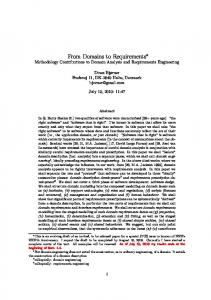
The purpose of this work is to evaluate and compare, by means of a common case study, two different testing methods for object-oriented software: a statistical testing method [Thévenod-Fosse et al. 1995] developed at LAAS-CNRS and a formal testing method [Barbey et al. 1996] [Péraire et al. 1998] developed at EPFL. For this purpose we propose the development of an object-oriented application of medium size, addressing all the phases of the software life-cycle: requirements, analysis, design, formal description, implementation and testing. Analysis and design are performed with the Fusion method [Coleman et al. 1994], formal description with the CO-OPN language [Biberstein et al. 1997], implementation with Ada 95 and testing with the two testing methods. The common case study chosen for this work is the production cell, originally defined in [Lewerentz and Lindner 1995]. Statistical test inputs
Informal Requirements
Analysis and Design Fusion
Formal Description CO-OPN
Implementation Ada 95
Formal test inputs
Fig. 1: Case study development life-cycle We have chosen Ada 95 as the implementation language, but it could be any other objectoriented language. However this choice will influence the test phase.
2.1
Fusion
Fusion [Coleman et al. 1994] is presented as a second-generation object-oriented development method, which covers all aspects of the software construction life-cycle and includes strategies for consistency checks. It is called Fusion because it synthesizes the best features of the prominent object-oriented development methods: OMT/Rumbaugh [Rumbaugh et al. 1991], the Booch method [Booch 1994], Objectory [Jacobson et al. 1994], and CRC [WirfsBrock et al. 1990]. It also includes some aspects coming from formal specification methods such as the Z method [Spivey 1992]. Throughout the whole development, a data dictionary is maintained to collect and check the consistency of the items introduced in the various models, together with some additional information, such as assertions on parts of the models or the initial values of the attributes. 2.1.1
Analysis
Fusion development starts with an analysis phase, in which the developer elaborates the object model, the system interface and the interface model. The object model describes the different classes of the system, their attributes and their associations in a fashion similar to entity-relationship diagrams [Chen 1976]. Among the
relationships, one can find the traditional relationships found in other methods such as inheritance (subtyping), aggregation, and association. The system interface consists of a full description of the set of operations to which the system can respond, of the events that it can output, and of the list of agents that can interact with the system. The interface model consists of the description of a life-cycle model and an operation model. The life-cycle model defines the possible sequences of interaction in which a system can participate. It lists the various events they can send to and receive from the system, together with their arguments. The operation model defines the effect of each system operation. This description includes some formal semantics in the form of pre- and postconditions. However, the semantics of these conditions are not very rigorous, since their definitions are not completely formalized. 2.1.2
Design
During design, the developer transforms the abstract models produced during analysis into software structures. In this phase, the developer must provide object interaction graphs, visibility graphs, inheritance graphs, and finally class descriptions. The object interaction graphs assign each system operation described in the operation model to a class and describe a decomposition of their behavior by distributing their functionality across various objects of the system. The visibility graphs show how the system is structured to enable inter-object communication. The inheritance graphs complete the domain-related subclassing relationships already found during analysis by including some information on inheritance in the implementation. Finally, the developer has to gather information coming from all these models and from the data dictionary to write a description of each class in the system. This class description is the first step in coding the application. All information regarding the specification of each class is given: its various attributes, including their type and visibility information, and its operations, including their various parameters and their result type. During the implementation phase, the programmer’s job is to implement the class descriptions in the target language, and code the behavior of each method according to the descriptions of the interface model, the operation model, and the interaction graphs.
2.2
Statistical Testing
Testing involves exercising the software by supplying it with input values. Since exhaustive testing is not tractable, the tester is faced with the problem of selecting a subset of the input domain that is well-suited for revealing the (unknown) faults. The selection is guided by test criteria that relate either to a model of the program structure or a model of its functionality, and that specify a set of elements to be exercised during testing (see e.g. [Beizer 1990]). For example, the control flow graph is a classical structural model, and branch testing is an example of a criterion related to this model. Given a criterion, the usual method for generating test inputs
proceeds according to the deterministic principle which consists in selecting a priori a set of test inputs such that each element is exercised at least once; and this set is most often built so that each element is exercised only once, in order to minimize the test size. But a major limitation is due to the imperfect connection of the criteria with the real faults: exercising only once, or very few times, each element defined by such imperfect criteria is not enough to ensure a high fault exposure power. To make an attempt at improving current testing techniques, one can cope with imperfect criteria and compensate their weakness by requiring that each element be exercised several times. This involves larger sets of test inputs that may be tedious to derive manually; hence the need for an automatic generation of test inputs. This is the motivation of statistical testing designed according to a criterion (see e.g. [Thévenod-Fosse et al. 1995]): combine the information provided by imperfect criteria with a practical way of producing numerous input patterns, that is, a random generation. In this approach, the probability distribution from which the test inputs are randomly drawn is derived from the criterion retained. Then it may have little connection with actual usage (i.e. operational profile): the focus is bug-finding, not reliability assessment. Also, the approach should not be confused with blind random testing, which systematically uses a uniform profile over the input domain [Duran and Ntafos 1984]. The statistical test sets are defined by two parameters, which have to be determined according to the test criterion retained: (i) the test profile, or input distribution, from which the inputs are randomly drawn and, (ii) the test size, or equivalently the number of inputs that are generated. As in the case of deterministic testing, test criteria may be related to a model of either the program structure, which defines statistical structural testing, or of its functionality, which defines statistical functional testing. The determination of the test profile is the corner stone of the method. The aim is to search for an input probability distribution that is proper to exercise each element defined by the criterion within reasonable testing times. Given a criterion C, let Sc be the corresponding set of elements, and Pc be the occurrence probability per execution of the least likely element of Sc. Then, the profile must accommodate the highest possible value for Pc. Depending on the complexity of this optimization problem, the determination of the profile may proceed either in an analytical (see e.g. [Thévenod-Fosse et al. 1991]) or an empirical way [Thévenod-Fosse and Waeselynck 1993]. The first way supposes that the activation conditions of the elements can be expressed as a function of the input parameters: then their probabilities of occurrence are a function of the input probabilities, facilitating the derivation of a profile that maximizes the frequency of the least likely element. The empirical way consists in instrumenting the software in order to collect statistics on the numbers of activation of the elements: starting from a large number of inputs drawn from an initial distribution (e.g. the uniform one), the test profile is progressively refined until the frequency of each element is deemed sufficiently high. Then the test size N must be large enough to ensure that the least likely element is exercised several times under the test profile inferred from the previous step. The notion of test quality qN provides us with a theoretical framework to assess a minimum test size, using Relation (1) which can be explained as follows: (1-Pc)N is an upper bound of the probability of never exercising some element during N executions with random inputs. Then, for a required upper
bound of 1-qN, where the target test quality qN will be typically taken close to 1.0, a minimum test size is derived. Nmin = ln(1-qN) / ln(1-Pc)
(1)
It is worth noting that Relation (1) establishes a link between qN and the expected number of times, denoted n, the least likely element is exercised: n ≅ - ln(1-qN). For example, n ≅ 7 for qN = 0.999. Returning to the imperfect connection of the criteria with real faults, it must be understood that the criterion does not influence random inputs generation in the same way as in the deterministic approach: it serves as a guide for defining an input profile and a test size, but does not allow for the a priori selection of a subset of input patterns. The efficiency of the probabilistic approach relies on the assumption that the information supplied by the criterion retained is relevant to derive a test profile that enhances the program failure probability. The main conclusion arising from previous theoretical and experimental work conducted on procedural programs (see e.g. [Thévenod-Fosse et al. 1995]) was that statistical testing is a suitable means to compensate for the tricky link between test criteria and software design faults. This imperfect connection is expected to get even worse in the case of OO programs, thus justifying further work addressing the statistical testing of OO software systems. As a first step, a feasibility study of statistical structural testing in cases of small OO programs was performed [Thévenod-Fosse and Waeselynck 1997]. The idea was to combine path selection techniques with the consideration of one specific OO concept: inheritance. This preliminary study allowed us to identify a number of problems, and on-going research work is now concentrated on two fundamental questions: first, how to define the unit and integration testing levels for OO software systems? and, second which software models and associated test criteria should be used as guides for designing statistical test patterns? The work presented in section 5 of this paper is mostly related to the second question, emphasis being put on statistical functional testing based on the models got from the analysis phase of Fusion.
2.3
CO-OPN
CO-OPN (Concurrent Object-Oriented Petri Nets) is a formalism for the specification and design of large OO concurrent systems [Biberstein et al. 1997]. Such systems consist of a number of objects which communicate by triggering parameterized events (sending messages). The external events to which an object can react are also called its methods. The behavior of the objects of a class are described by algebraic Petri nets. Cooperations between objects are described by synchronization expressions: each event may request a synchronization with some method invocations of one or several other objects. A CO-OPN specification consists of a collection of two kinds of entities: algebraic data types (ADT modules) and classes. ADT modules are used to specify or reuse primitive data types such as integers or booleans or more elaborated data types such as lists or queues. Class modules are used to define encapsulated objects with an internal state and some methods which
provide the environment with various services. An example of a CO-OPN class module is given in section 6.1. It is made of an interface and a body. The body describes the typed places and the internal transitions of the algebraic Petri net, and its behavior by some behavioral axioms; moreover, it may specify some synchronization with other objects. Synchronization expressions use three operators: "//" for simultaneity, ".." for sequence, and "+" for alternative. The general form of behavioral axioms, where [] denotes some optional component, is: Event [With SynchroExpression] :: [Condition] ⇒ Precondition → Postcondition Event is the name of a method, with possibly some parameters, or an internal transition. The With key word introduces a synchronization requirement: the event can occur if and only if the
method invocations of the synchronization expression can be performed. The part after "::" describes the effect of the event using the data types specified in the ADT modules. The Precondition and Postcondition respectively express what ADT values are consumed and produced in the concerned places of the net.
2.4
Formal Testing
This approach is an adaptation to OO systems of the BGM method [Bernot et al. 1991], a theory of testing developed at LRI for testing data types by using formal specifications. The formal testing method is an approach to reveal faults in a program by verifying its functionalities without analyzing the details of its code. The goal is to answer the question: "Does a program satisfy its formal specification?", or, in accordance to the goal of testing, to find if a program does not satisfy its specification. This kind of testing aims at revealing faults in a program by comparing it against a specification. It is usually decomposed into the following three phases: (i) a test selection phase, in which some test cases that express properties of the specification are generated, (ii) a test execution phase, in which the test cases are executed and the results of the execution collected and, (iii) a test satisfaction phase, in which the results obtained during the test execution phase are compared to the expected results. The formal testing process is shown in figure 2. Does the program P satisfy the specification SP?
Test Requirement
Test cases generation from SP
Test Selection
Test cases execution on P
Test Execution
Test procedure
Program Correction Comparison with expected results
Yes — No — Inconclusive
Fig. 2: Formal testing procedure
Test Satisfaction
Test Interpretation (Verdict)
The test selection phase starts with an infinite set of formulae, corresponding to all the properties required by the specification. This infinite set is reduced into a finite set of formulae which is sufficient, under some hypotheses, to state the preservation of these properties. The infinite set of formulae is called the exhaustive test set T0. The reduction of the exhaustive test set to a finite test set is performed by applying hypotheses Hk to the program (see figure 3). Those hypotheses, called reduction hypotheses and presented in section 6.2.1, define selection strategies and reflect common test practices.
Application of hypotheses
H0
T0
...
...
Hi
Ti
Hj
Tj
...
...
H
T
Reduction of the test set
Fig. 3: Test selection process Consequently, given a program P, its specification SP and some reduction hypotheses H on the behavior of P, the idea of the test set selection procedure is to find some T of reasonable size such that, if P satisfies H, we have an equivalence between the satisfaction of the test T by P, and the satisfaction of the specification SP by P: (P satisfies H) ⇒ (P satisfies T ⇔ P satisfies SP). In formal testing, specification and test sets can be expressed using different languages: a specification language well adapted to the expression of properties from an user point of view, and a test language well adapted to describe test cases from a tester point of view. In our case, specifications are written in CO-OPN (see section 2.3), and test sets are written using Hennessy-Milner Logic (HML) [Hennessy and Milner 1985]. HML is a temporal logic having the not (¬), the and (∧) and the next (< >) operators. This logic allows to express tests detecting problems related to sequentiality and concurrency, such as wrong internal nondeterministic choices. There is a full agreement between these two languages, i.e. the satisfaction of the temporal formulae is preserved for the implementations of a given specification [Péraire 1998]. An elementary test for a program under test P and a specification SP is defined as a couple where: •
Formula ∈ HMLSP: (ground) temporal logic formula
•
Result ∈ {true, false}: boolean value showing whether the expected result of the evaluation of Formula (from a given initial state) is true or false with respect to the specification.
A test is successful if Result reflects the validity of Formula in the labeled transition system modeling the expected behavior of P. In all other cases, a test is a fail. It is important to note that the test definition will allow the test procedure to verify that a non-acceptable scenario cannot be produced by the program. An advantage of this approach is to have an observational description of the valid implementation through the tests. One test is a formula which is valid or not in the specification and that must be experimented in the program i.e. a correct implementation behaves as described in the tests. Interested readers will find further information about this formal testing method in [Barbey et al. 1996], [Péraire et al. 1998], [Barbey 1997] and [Péraire 1998].
3
Presentation of the case study
The aim of this case study is to develop a control program for an existing industrial production cell, taken from a metal-processing plant in Karlsruhe (Germany). This case study was launched by FZI (Forschungszentrum Informatik) in 1993, within the German Korso Project, to evaluate and compare different formal methods and to show their benefits for industrial applications. At the moment, the production cell case study has been investigated by more than 35 different research groups. This is an industry-oriented problem where safety requirements play a significant role, as the violation of a requirement might result in damage of machines or injury to people. Also, this is a reactive system, as the control program has to react permanently to changes in its environment. Moreover, this application was chosen because the control program can be modeled as a collection of cooperative concurrent agents. This section is a summary of the presentation of the case study given in [Lewerentz and Lindner 1995].
3.1
Description of the Cell
The production cell is composed of six machines: two conveyor belts (feed belt and deposit belt), a travelling crane having an extendable arm equipped with an electromagnet, an elevating rotary table, a press and a rotary robot having two orthogonal extendable arms equipped with electromagnets (see figure 4). The aim of the cell is the transformation of metal blanks into forged plates (by means of a press) and their transportation from the feed belt into a container. The production cycle of each blank is the following (see figure 4): •
the feed belt conveys the blank to the table,
•
the table rotates and rises to put the blank in the position where the robot is able to magnetize it,
•
the first robot arm magnetizes the blank and places it into the press,
•
the press forges the blank,
•
the second robot arm places the resulting plate on the deposit belt,
•
the crane magnetizes the plate and brings it from the deposit belt into a container. deposit belt (belt 2) upper arm (arm 1)
travelling crane
robot press
lower arm (arm 2)
container
electromagnets
elevating rotary table up / down
feed belt (belt 1) Fig. 4: Top view of the production cell
Note that in the original case study proposed by FZI, the crane magnetizes the plate and brings it from the deposit belt back to the feed belt; this is in order to perform the demonstration without an operator. In the real cell, the crane is not between the two belts, but links the cell with another manufacturing unit (modeled in our case by a container). In this paper we will focus on the robot because it is the most complex device of the production cell. See [Barbey et al. 1998] for a complete description of the cell. • Description of the Robot Potentiometer
electric motor
(0..1)
electromagnet Potentiometer electric motor
(-100..70)
Fig. 5: Robot (side view)
The rotary robot (see figure 5) consists of two orthogonal extendable arms equipped with electromagnets. The robot is powered by three bidirectional electric motors which allow the rotation of the robot and the horizontal translation of the arms (extension or retraction). The motors can be started and stopped by the control program. The rotation angle of the robot and the amount of extension of each arm are given by potentiometers. In order to meet various safety requirements, each arm has to be retracted while the robot rotates and while the other arm loads or unloads a blank.
3.2
Control Program and Simulator
The control program receives information from the cell by means of three kinds of sensors: switches, photoelectric cells, and potentiometers. The control program controls each machine of the cell by means of actuators. To allow the evaluation of the control programs of the different research groups, the FZI (Forschungszentrum Informatik) provides a simulator which imitates the important abilities of the real production cell. The FZI simulator is managed by transmitting commands to it and receiving sensor informations from it. It performs the movements of the devices and blanks, detects collision and reports them by mean of the error list. We use a modified version of the FZI simulator in which each metal plate ends its cycle in the cell into a container. In our study we make the assumption that the simulator works properly.
3.3
Safety Requirements
Safety requirements play a significant role in the context of reactive systems: if a safety requirement is violated, this might result in damage of machines or injury to people. This section presents examples extracted from the production cell’s 21 safety requirements. Requirement 1. The robot must not be rotated clockwise if arm 1 points towards the table, and it must not be rotated counterclockwise if arm 1 points towards the press. Requirement 9. The robot having an arm in the proximity of the press may only rotate if this arm is retracted. Requirement 18. A plate may only be put on the deposit belt if the deposit belt photoelectric cell confirms that the preceding plate has arrived at the end of the deposit belt. Requirement 21. If the table is loaded, the robot arm 1 may not be moved above the table if it is also loaded (otherwise the two blanks collide).
4
Analysis and design of the case study with the Fusion method
This section presents pieces of the Fusion [Coleman et al. 1994] analysis and design of the production cell controller. In particular, the parts related to the robot are presented in detail.
4.1
Analysis
The Fusion analysis produces a declarative specification of what the system does, by means of a system context diagram, an object model, a system life-cycle and operation models.
4.1.1
System Context Diagram
Figure 6 shows an inside view of the controller. Since the controller is a concurrent system, it has been separated — as proposed in section 3.5 of the Fusion handbook [Coleman et al. 1994] — in order to view it as a set of cooperating agents, each of which being developed using Fusion. The inside view of the controller mimics its environment: to each device of the production cell corresponds an agent of the controller. The incoming and outgoing events between devices and agents are not shown in figure 6. The events TurnOn and TurnOff are sent by the operator to all agents of the controller (for creating and initializing them), and are not represented either. Controller
Table
go_unload_position pick_from_table feed_table
FeedBelt
go_load_position load_press pick_from_press
Press
Robot go_load_position forge deposit_on_belt
add_blank
Operator
bring_past_end
Crane
DepositBelt pick_from_belt
Fig. 6: System context diagram (Inside) The significance of the arrows is the following: to each arrow corresponds an asynchronous event, i.e. the event will be sent even though the receiving agent is not ready to treat the event. Events are blocking, i.e. the sending agent is blocked until the receiving agent is able to treat the event. The principle behind event generation is that every agent is autonomous: it will do as many actions as it can independently. The Fusion documents [Coleman et al. 1994] do not state how a set of cooperating agents, each of which being developed in Fusion, interact. It is clear that it is via events, since the interface model and, partially, the operation model rely upon emissions of events. But the behavior of an agent when receiving an event is not described. It is somewhat normal since in the sequential case addressed by these documents agents are external to the analyzed and designed system. It would not be realistic to assume anything about them. In our case, concurrent agents have been developed in Fusion, as suggested in [Coleman et al. 1994]. We considered the possibility to follow the Fusion rule for sequential systems, that is input events are ignored when the system is not ready to treat them. However, for such a concurrent controller it would introduce unnecessary complexity in the analysis. Consequently, our analysis rely upon the following assumption: if at any point an agent of the controller receives an event, it queues it and will treat it when possible (see section 4.1.3). Furthermore, this principle is directly supported in our implementation by the Ada95 rendezvous mechanism.
4.1.2
Object Model
The object model describes the different classes of the system, their attributes and their associations. Thus the controller object model is composed of one object model per agent. These different object models are interconnected by means of associations. Figure 7 shows the robot object model (disconnected from its environment) as an aggregate including its sensor (a potentiometer) and its actuators (a motor and two arms). Similarly, each robot arm is an aggregate including a sensor (a potentiometer) and two actuators (a motor and an electromagnet). Robot arm1_pick_extension, arm1_pick_retraction arm1_drop_extension, arm1_drop_retraction arm2_pick_extension, arm2_pick_retraction arm2_drop_extension, arm2_drop_retraction 2
Arm Bidirectional_Electric_Motor status progression, retrogression stop Potentiometer name value
Potentiometer name value
Electro_Magnet status action, inaction
Bidirectional_Electric_Motor status progression, retrogression stop
Fig. 7: Object model of the Robot
4.1.3
System Life-Cycle
The life-cycle model defines the allowable sequences of event treatments in which an agent may participate. If at any point the agent receives an event that is not allowed according to the life-cycle, then the system queues it and the state of the sending agent remains unchanged. Note that the order of the event treatments does not always correspond to the order of the event receptions into the waiting queue: an events reordering could be done by the program. The life-cycle model is defined in terms of regular expressions. The regular expressions consist of events and the operators of concatenation “.”, alternation “|”, repetition “*” for zero or more occurrences, “+” for one or more occurrences, interleaving “||”, optionallity “[ ]”, and grouping “ ( )”. In decreasing order, the precedence is [ ], *, +, . , | , || . Expressions are grouped to override default precedence. The controller life-cycle is composed of the life-cycles of the different agents of the system. Below are the life-cycle schemata for the robot and controller:
lifecycle Robot :
initialize . EmptyRobot
lifecycle EmptyRobot : ( pick_from_table . #go_load_position . Arm1 | pick_from_press . #go_load_position . Arm2 )* lifecycle Arm1 :
( load_press . #forge . EmptyRobot | pick_from_press . #go_load_position . Arm12)*
lifecycle Arm2 :
( pick_from_table . #go_load_position . Arm12 | deposit_on_belt . EmptyRobot )*
lifecycle Arm12 :
( load_press . #forge . Arm2 | deposit_on_belt . Arm1 )*
lifecycle Controller: TurnOff
TurnOn . (FeedBelt || Table || Robot || Press || DepositBelt || Crane) .
EmptyRobot, Arm1, Arm2
and Arm12 correspond respectively to the state of a robot carrying no plate, one plate with the first arm, one plate with the second arm and one plate in each arm. 4.1.4
Operation Models
The operation model defines the behavior of the system by specifying how each operation affects the system state. Each specification includes informal preconditions (Assumes) and postconditions (Result) that describe the effect of the operation on the object model. Objects that the Result clause indicates as either created or modified are listed in the Changes field. Any message that may be sent to agents as a result of invoking the operation are listed in the Sends field. Below are presented two robot operations: pick_from_table and deposit_on_belt. Operation:
pick_from_table
Description:
Pick up a plate from the table.
Changes:
The first robot arm carries a plate (the magnet is on). The first robot arm is retracted and points toward the table.
Sends:
Table: {go_load_position}
Assumes:
The table is in unload position. The table is loaded. The first robot arm is free (the magnet is off).
Result:
The first robot arm carries a plate (the magnet is on). The first robot arm is retracted and points toward the table. An event go_load_position has been sent to the table.
Operation:
deposit_on_belt
Description:
Deposit a plate on the deposit belt
Changes:
The second robot arm holds no plate (the magnet is off). The second robot arm is retracted and points towards the deposit belt.
Sends:
—
Assumes:
The second robot arm holds a plate (the magnet is on). There is no plate at the beginning of the deposit belt.
Result:
The second robot arm holds no plate (the magnet is off). The second robot arm is retracted and points towards the deposit belt.
4.2
Design
The Fusion design produces an abstract OO model of how the system realizes the behavior required by the analysis, mainly by means of interaction graphs and class descriptions. 4.2.1
Interaction Graphs
An object interaction graph is constructed for each operation of the operation models to show which objects are involved in the computation and how they cooperate to realize the functionality required by the analysis. Below are presented the textual descriptions of the interaction graph of two robot operations: • Robot operation pick_from_table Operation Robot: pick_from_table () - move the robot so that the first arm is in front of the table, - extend the first arm over the table, by an amount given in the attribute arm1_pick_extension, - pick up the plate, - retract the first arm from the table, by an amount given in the attribute arm1_pick_retraction, - send go_load_position to the table.
Note that go_load_position corresponds to an output message sent to the table. • Robot operation deposit_on_belt Operation Robot: deposit_on_belt () - increment by 1 deposit_on_belt_counter i.e. the number of blanks the robot can drop on the deposit belt. Deposit_on_belt is the only event for which the state of the sender can change before the end of the treatment: the design makes it non-blocking.
The real dropping is done by an internal method deposit_on_belt_int which is automatically called when the robot is ready to drop a plate on the deposit belt. This mechanism prevents deadlock situations between the robot and the deposit belt. Indeed, the method deposit_on_belt_int ensures that the deposit belt is never blocked waiting for the robot, and the counter deposit_on_belt_counter ensures that the robot always knows how many blanks can be dropped on the deposit belt. • Robot method deposit_on_belt_int Method Robot: deposit_on_belt_int () if deposit_on_belt_counter > 0 then - move the robot so that the second arm is in front of the deposit belt, - extend the second arm over the deposit belt, by an amount given by arm2_drop_extension, - drop the plate on the deposit belt, - retract the arm from the deposit belt by an amount given in the attribute arm2_drop_retraction, - decrement by 1 the number of blanks the robot can drop on the deposit belt.
It is interesting to note that the preceding mechanism (induced by the method deposit_on_belt_int and the counter deposit_on_belt_counter) was not present in the first version of our Fusion modeling. The need for this mechanism has been revealed by the test phase (see Section 5.2.5 and section 6.3.1.2).
4.2.2
Class Descriptions
A class description is produced for each class mentioned in the object interaction graphs. A class description is a textual summary of the design decisions that affect the implementation of a class. Below is presented the description of the class Robot: Robot class Robot // data attributes attribute constant arm1_pick_extension: Extension := 0.5208 attribute constant arm1_pick_retraction: Extension := 0 attribute constant arm1_drop_extension: Extension := 0.6458 attribute constant arm1_drop_retraction: Extension := 0.3708 attribute constant arm2_pick_extension: Extension := 0.7971 attribute constant arm2_pick_retraction: Extension := 0 attribute constant arm2_drop_extension: Extension := 0.5707 attribute constant arm2_drop_retraction: Extension := 0 attribute constant deposit-on-belt_counter: Number_Blanks := 0 // references // exclusive bound: // object attribute used exclusively by robot // and having a lifetime bound to the lifetime of a robot. // shared unbound: // object attribute shared by different classes and having an unbound lifetime. attribute constant arm1: exclusive bound Arm attribute constant arm2: exclusive bound Arm attribute constant rotation_motor: exclusive bound Bidirectional_Electric_Motor attribute constant rotation: exclusive bound Potentiometer attribute constant table: shared unbound Table attribute constant press: shared unbound Press attribute constant depositbelt: shared unbound DepositBelt // creation methods method create () // public methods method deposit_on_belt () method initialize () method load_press () method pick_from_press () method pick_from_table () // private methods method move (p: Robot_Position) method deposit_on_belt_int () method deposit-on-belt_init () method deposit-on-belt_increment () method deposit-on-belt_decrement () endclass
5
Statistical Testing based on Fusion
5.1
Overview of the approach
Statistical functional testing consists in basing the probabilistic generation of test patterns on the black box analysis of the program under test. For this, a general approach is to make use of available information got from the adopted development method. For example, previous work on procedural programs [Thévenod-Fosse et al. 1995] based the design of statistical testing on the behavioral models that accompany SA/RT development (namely, finite state machines and decision tables). The production cell case study allowed us to study how this general approach can be applied in the case of object-oriented development methods, taking the example of the Fusion method. The design of statistical testing was then based on two kinds of information from the case study documentation [Barbey et al. 1998]: the list of 21 safety requirements, and the models got from the analysis phase of Fusion. Classical development methods for procedural programs involve a hierarchical decomposition of functions. On the contrary, OO development methods are characterized by decentralized architectures of objects. The traditional unit and integration levels of testing do not fit well in this case. Unit testing of functions cannot be mapped onto testing of individual object's operations: taken in isolation, the body of one operation typically consists of a few lines of code; its behavior is meaningless unless analyzed in relation to other operations and their joint effect on a shared state. Hence, any significant unit to be tested cannot be smaller than the instantiation of one class. Moreover, as pointed out in [Kung et al. 1995], the many relationships that exist in an OO program (inheritance, aggregation, client/server relationships, …) imply that one class inevitably depends on another class. It is difficult to determine where to start testing, and there is no obvious order for an integration strategy. To determine the testing levels, we considered the possibility of associating a functional description with a (set of) class(es): •
The unit level corresponds to small subsystems that are meaningful enough to have interface models in Fusion, that is, a life-cycle and an operation model. From Section 4, there are six such subsystems: the feedbelt, the table, the robot, the press, the deposit belt and the crane. Each of them is already an aggregation of classes. This means that the basic classes will not be tested in isolation. For example, there is no specific unit testing of the Electro_Magnet class: this basic class will be tested through its embodying subsystems, namely the robot and the crane.
•
The integration process is guided by the consideration of the safety requirements. For example, requirement 21 (see Section 3.3) led to the definition of an integration test for the subsystem robot+table. Four integration tests and one system test were thus defined.
The respective focus of each testing level (unit, integration) was determined in order to define a cost-effective test strategy for reusable components. The concern is to identify what can be tested once for all at the unit level and what has to be tested during the integration process specific to each application. Since it is well-recognized that a component that has been
adequately tested in a given environment is not always adequately tested for any other environment, emphasis was put on designing unit testing without making any assumption on the operational context of the component. As a result, a component that passes the unit test phase should be robust enough to be used in any context without requiring further unit testing; and testing may be focused on the verification of application-specific requirements for subsystems integrating the reused component. If a component is not robust enough to pass the unit test phase, assumptions that govern its correct behavior can be identified from the results of unit testing. Whether or not these assumptions hold in a given application context has then to be verified during the integration process. Then, unit testing was mainly focused on verifying conformance to interface models. Let us recall that the life-cycle defines the allowable sequences of event treatment, implying a reordering of events by the receiving subsystem, while the operation model describes the effects of each event treatment. The target subsystems were placed in an “hostile” environment: there was no timing or sequence assumptions related to the events sent to the subsystem. This allowed us to verify the correct reordering of events, and the correct treatment of the reordered events, in response to arbitrary solicitations. The design of integration testing was focused on the verification of safety properties of the production cell, taking into account some characteristics of this application. This led to a more constrained version of the input environment. For example, when testing the subsystem robot+table, it was not possible to sent a new load_press event to the robot while the previous one had not yet been treated. This was so because we know that the robot is connected to a single press, and that press is blocked until the previous load_press is treated. In this paper, emphasis is put on unit testing (Section 5.2). Then Section 5.3 outlines the integration testing process.
5.2
Unit testing
The unit testing process can be decomposed into phases that accompany the Fusion development phases. The main objective was to verify the conformance of the units to their interface models in an “hostile” environment. This general objective had first to be refined: the choice of a conformance relation and of test coverage criteria is performed by considering the high-level Fusion analysis of the target components (Sections 5.2.1 to 5.2.2). Then the development of a test environment supporting the refined objective (Section 5.2.3) should accompany the later phases of Fusion: as exemplified by the production cell case study, the ability to handle a number of controllability and observability problems is strongly dependent on the design and implementation of the unit under test. The test environments implemented for the target units made it possible to apply the statistical test sets designed for them (Section 5.2.4). Several faults were revealed (Section 5.2.5). 5.2.1
Oracle
The role of the oracle is to determine conformance of the test results to the expected ones: when no discrepancy is observed, the program is considered to be correct. Hence, the
stringency of the notion of correctness is highly dependent on the oracle procedure, that is, on the granularity of the definition of the expected results. According to the goal of unit testing, the oracle of each unit was defined as being composed of: •
the life-cycle of the unit under test,
•
the postconditions of the operation model of the unit under test,
•
the safety requirements related to the unit under test taken in isolation.
From the 21 safety requirements listed in [Barbey et al. 1998], 15 were included in the unit oracle procedures thus defined. For example, six requirements are related to the robot behavior: five of them are part of the robot oracle, the last one being ignored because it is deemed not checkable (“Both robot arms must not be retracted or extended more than necessary ”). The checks related to conformance to the life-cycle and operation models were determined according to a thorough examination of the Fusion analysis of the production cell. 5.2.2
Examination of the Fusion analysis models with a view to testing
The examination of the life-cycle and of the operation model associated to each unit was performed with the double aim of 1) choosing coverage criteria based on the models; 2) identifying the information to be observed in order to implement oracle checks. • Coverage criteria based on the models The life-cycle model specifies the order in which each unit should process input events and send output events. The processing of input events is made more precise in the operation model, where, in particular, preconditions (Assumes) and postconditions (Results) are stated. The textual life-cycle expression can be put into an equivalent form: a finite state automaton recognizing the corresponding regular expression. However this automaton is not sufficient to describe the allowed sequences of processed events, because no operation should be triggered outside its precondition. Then, the set of allowed sequences should be further constrained by considering whether the postcondition of one operation implies the precondition of the next one. According to the Fusion method, a condition that has to be true both before and after the operation is not listed, neither as a precondition nor as a postcondition; and the granularity of the operation model does not distinguish between the case where the condition remains true throughout the operation execution, and the case where it turns to false and then returns to true before the end of the operation. In both cases, from the test viewpoint, it is important to check the validity of the condition after completion of the operation. As a result, a completed version of the operation model was provided for testing purpose, in which both preconditions and postconditions are expanded. For example, in the operation model of the robot operation pick_from_table (see Section 4.1.4), the three following preconditions and postconditions were
added: the rotation motor is off, the lower arm’s translation motor is off, the upper arm’s translation motor is off. Combining the information got from the life-cycle expression and the completed operation model, the allowed sequences of event treatment for each unit are reformulated as finite state automata. As an example, a reformulation of the robot life-cycle is provided in Figure 8. The textual life-cycle expression would have given us a 4-states automaton, depending on which arm is carrying a plate. The examination of the operation model shows that presence or absence of a plate in the press should also be taken into account: the robot is not allowed to process operation pick_from_press if it did not previously load the press. deposit_on_belt
initialize
Empty
pick_from_table #go_load_position elt
_b
on
t_ osi
p
de
Arm12
load_press #forge
Arm1
load_press #forge
pick_from_press #go_load_position #g
de
Arm2 pick_from_table Press #go_load_position
Arm2
pic k_ loa from d_ po _tab l sit ion e
o_
lt be
n_
t_o
si po
Press
Arm12 deposit_on_belt Press
Arm1 Press
pick_from_press #go_load_position pick_from_table #go_load_position
Fig. 8: Robot life cycle automaton A finite state automaton is a very classical model to derive functional test data: a number of coverage criteria have been defined in the literature. Previous work on statistical testing showed that the most cost-effective approach should be to retain weak criteria facilitating the search for an input distribution and to require a high test quality wrt them. Hence we retained the weak criterion of transition coverage while requiring a test quality of qN = 0.999. As explained in Section 2.2, this test quality implies that the least likely transition should be exercised 7 times on average by a given test set. Since the initialization transition is one of the transitions to be exercised, it can be deduced that one test set has to be composed of several sequences of input events, each one starting by initialize. The coverage criterion for the automaton relates to the ability of the test set to trigger the internal treatment of input events in various state configurations. However, it says nothing about the coverage of the event reordering functionality to be supplied by the unit. Hence, it has to be supplemented by another criterion forcing the input sequences to be sufficiently “arbitrary” to trigger the reordering mechanisms of event processing. Input events are supposed to be stored in a waiting queue if the unit is not ready to process them. Then this queue may be characterized by the number of events of each category (e.g. pick_from_table, pick_from_press, load_press, deposit_on_belt) that are waiting to be processed. The retained criterion is the coverage of four classes of queue configurations for each category of event: the number of queued events
of that category is 0, 1, 2 or 3.We required the same test quality as previously, namely qN = 0.999. It is worth noting that controlling coverage of these various elements is not trivial. The internal behavior of one unit depends not only on the order in which events are received, but also on the interleavings of event reception and event treatment. • Event interleavings To illustrate the problem, let us assume that some test sequence first takes the robot to the Arm12 state (see Figure 8) with no queued event, and then is continued by subsequence load_press.deposit_on_belt.pick_from_table. Then, for this sequence of events, the robot behavior may be different depending on the triggered interleaving (see Figure 9). load_press deposit_on_belt
load_press treatment of load_press
treatment of load_press
pick_from_table
deposit_on_belt
treatment of deposit_on_belt
treatment of pick_from_table pick_from_table
(a)
(b)
Fig. 9: Different possible interleavings for a same sequence of events If the time intervals between the three events are such that none of them is received before the previous one has been processed (interleaving 9a), then deposit_on_belt is processed before pick_from_table and the queue remains empty. If both deposit_on_belt and pick_from_table are received before completion of the load_press operation (interleaving 9b), then one of these events is queued and the other processed depending on some implementation choice. Hence, the triggered behavior in terms of transition coverage and queue configuration coverage may be quite different for two interleavings of the same sequence of events. It is not possible to know in advance the exact duration of one operation: the best that can be done is to estimate a conservative upper bound of this duration. Then, if the delays between input events are long enough compared to the reaction time of the units (synchrony hypothesis), the coverage supplied by a given test sequence can be assessed a priori, like in Figure 9a. But such a low load profile is not expected to be sufficient if the synchrony hypothesis does not hold in the operational context: other possible intervealings, like the one of Figure 9b, should not be excluded from the test input domain. For example, if the treatment of events is not atomic, it must be possible to trigger the reception of events during an on-going treatment. And irrespective of the atomicity hypothesis, it must be possible to trigger schemes where several concurrent events are received in the meantime between two treatments. As will be explained
in Section 5.2.4, this problem led us to introduce some notion of time in the definition of test sequences: several load profiles, i.e. time interval profiles, had to be considered. • Oracle checks for conformance to interface models The examination of interface models led us to reformulate the life-cycle of the units. It turns out that the resulting non-deterministic automata possess a remarkable property: for any test sequence, the final state and number of processed events at the end of the sequence does not depend on the non-deterministic choices made during the execution of the sequence. For example, the previous test sequence always takes the robot to the Arm12 state with an empty queue, irrespective of its intermediate behavior. Accordingly, the oracle conformance checks were specified as follows: •
the observed sequences of input events processed and output events sent must be recognized by the life-cycle automaton;
•
the number of events of each category that are processed by the unit is the same as the number of events that would be processed by the life-cycle automaton exercised with the same test sequence.
Appropriate information is to be monitored by the test environment. In particular, the feasibility of oracle checks depends on the availability of some ordering information concerning the treatment of input event and emission of output event. However, the reordering of input events according to the life-cycle is encapsulated in the units: once the input events have been received by a unit, the test environment may be unable to know the order of their internal treatment. This observability problem was taken into account in the design of our test environment (see Section 5.2.3). The completed operation models give us the postconditions to be checked during testing to verify the effect of the input event treatment. Note that in the case of the production cell, the postconditions relate to the state of the physical devices controlled and monitored by the software units (e.g. position of the robot arms, ...) rather than to the values of some internal program variables. In our test environment, their verification was implemented by instrumenting the FZI simulator used to mimic the reaction of the physical devices. Checking the postconditions also raises observability issues. Postconditions must be observed just at the end of the corresponding operation execution and before potential state evolution due to another operation. Hence, it must not be possible for a unit to process another event while the previous postcondition has not yet been checked. 5.2.3
Test environment
The design of the unit test environment was guided by the previous analysis. Accordingly, a number of controllability and observability problems had to be solved. While the test objective was refined by considering only the Fusion analysis models, the development of a test environment supporting this objective required the Fusion design and Ada implementation to be taken into account. A general view of the resulting test environment is provided in Figure 10. The corresponding design choices are justified below.
termination repor t
Auxiliary drivers sending events to the unit (1 auxiliary driver per event)
Creation and initialization
Main driver
Creation and initialization
Input event (driver blocked until event treatment)
Unit under test
Commands and status requests
Output event
status
Stubs receiving output events and activating the verification of observable post-conditions
verification requests
Tcl/Tk simulator
Fig. 10: Test environment at the unit level • Design choices wrt controllability problems A test sequence is defined as a sequence of input events with time intervals between two successive events. Since there is no ordering assumption related to the events sent to the units, the test environment must be able to control any arbitrary input sequence. The examination of the Ada code shows that sending an input event to a unit corresponds to requesting a rendezvous. Then we must be careful not to introduce deadlocks when the event order departs from the one specified in the life-cycle. Let us take the example of a unit having a life-cycle defined as (E1.#e1.E2#e2)*, and exercised with an input sequence having order E2.E1. The expected behavior of the unit is to treat both events in the life-cycle order: the treatment of E2 is delayed until E1 has been processed and e1 has been sent. If the test driver is implemented by a single Ada task sequentially calling entries E2 and E1, then the driver is blocked on E2: E1 will never be sent. To handle this controllability problem, the adopted solution is to have the input events be sent by concurrent tasks. The main driver reads the input sequence, and successively creates one auxiliary driver per event to send to the unit under test. The time intervals defined in the test sequence represent delays between the creation of the two corresponding auxiliary drivers. Each auxiliary driver is a simple task sending its event to the unit, remaining blocked until the event is treated and then reporting successful termination to the main driver. The main driver ensures termination of the test experiment even in case of deadlock of the auxiliary drivers and the target unit. A deadlock is diagnosed when the main driver receives no termination reports during a predetermined time period. Note that a deadlock may be an expected result of the test experiment. Returning to the simple example given above, this would be the case for any test sequence containing a larger number of E2 events than of E1 events.
• Design choices wrt observability problems The examination of Fusion analysis models showed that both the beginning and end of operation executions should be made observable. Moreover, some ordering relations must be preserved by the results of (possibly concurrent) observers: for a given unit, observation of the beginning of one operation should always be reported before the end of this operation; postconditions checks must always be performed and reported before the beginning of the next operation of this unit. Two solutions can be considered. The first one is to adequately instrument the Ada code. The second one is less intrusive: synchronize the observation with the emission of output events, provided those events are sent by the unit at the beginning or end of the operation; let us recall that the state of the unit remains unchanged while its output event has not been processed (see Section 4.1.3), hence ensuring that no new event is treated in the meantime. The examination of the operation model shows that, in accordance with the life-cycles of the different agents, all the unit operations trigger output events, except five of them: the initialize operations of three units (feedbelt, robot, crane), the robot operation deposit_on_belt and the feedbelt operation add_blank. Then, the beginning and end of these 5 operations will not be observable unless special-purpose instructions are added in the Ada code. For the other operations, the granularity of the operation model does not allow us to determine when output events are sent. The answer is given by the interaction graphs of the Fusion design model (see Section 4.2.1): their review shows that sending output events always correspond to the last step of the operation descriptions. Back to the operation model, it is noticed that two different operations may involve the same output event, but then it turns out that the same postcondition is required from both operations. Accordingly, the adopted solution is the following: the beginning of each operation is observed through instrumentation of the Ada code (insertion of a print statement at the start point of the treatment), while the observation of postconditions is synchronized with the observation of output events. This design choice for the observers implies that the postconditions of the 5 operations with no output event are not observable. Furthermore, new observability problems were identified during the implementation of the unit test environments. Most of them are due to the limitation of the simulator: for example, there is no “forged” status available from the simulator for the metal blanks. But one problem is due to a discrepancy between the Fusion interaction graph of one robot operation and the corresponding Ada code: contrary to what was stated in the Fusion design (see Section 4.2.1), the go_load_position event is sent before the end of the pick_from_table operation, so that the post-condition related to the position of the first robot arm cannot be observed. • Implementation of the test environments The test environments resulting from these design choices are such that each test experiment generates a trace file recording:
•
the sequence of every event treated or sent by the unit under test. The treatment of an input event is observed owing to the existence of special-purpose instructions in the Ada code of the unit. The output events are observed by the stubs receiving them.
•
the number and category of input events not treated at the end of the test experiment. This information is generated by the main driver when a deadlock is detected.
•
the results of the checks for the status of the devices at the end of the operations. These checks are activated by the stubs when they receive an output event. The FZI simulator has been added a parametrized verification function that allows specific postconditions (position of a given device, presence of a metal plate on this device, ...) to be observed. By sending the appropriate request to the simulator, the stubs make it possible to verify the observable post-conditions got from the completed operation models, as well as to verify some safety requirements.
•
the error messages of the FZI simulator. The FZI simulator has built-in mechanisms to issue an error message in case of abnormal situations like collision of devices, or falling of metal plates.
Then this trace file is analyzed off-line by an oracle program in order to issue an acceptance or rejection report. One test environment has been implemented for each of the six units, based on the principle given in Figure 10. For example, the test environment of the robot is composed of the following elements: one main driver; four categories of auxiliary drivers corresponding to the input events of the robot (pick_from_table, pick_from_press, load_press, deposit_on_belt); one press stub receiving the output events go_load_position and forge; one table stub receiving the output event go_load_position; one deposit belt stub receiving no event. The verification function added to the FZI simulator, called by the stubs with proper parameters, allows us to observe every postconditions got from the completed operation models, except the ones related to operations with no output event (operations initialize and deposit_on_belt), and the one related to pick_from_table mentioned above. Five safety requirements were also observed from the simulator, including requirements 1 and 9 shown in Section 3.3. The oracle program takes as input the trace file of a test experiment, from which two kinds of information are extracted: (i) the error messages from the simulator checks, and (ii) the sequences of input event treatments and output event emissions that are analyzed according to the robot life-cycle automaton. 5.2.4
Design of statistical test patterns
A test sequence is defined as a sequence of input events with time intervals between two successive events. For each unit, statistical test patterns had to be designed according to the coverage criteria defined in Section 5.2.2, that is: (1) the transitions of the unit life-cycle automaton (see Figure 8 for the robot) and, (2) the four classes of queue configurations for each category of event.
Controlling coverage of these various elements is very difficult – or even, impossible – because the internal behavior of one unit depends on the interleavings of event reception and event treatment: as illustrated in Figure 9, different interleavings are possible for a same sequence of events depending on the delays between event emissions. As noted in Section 5.2.2, the coverage of the target elements supplied by a given test sequence can be a priori assessed only under the synchrony hypothesis, that is, assuming long delays which correspond to the kind of interleaving shown in Figure 9a. Hence, the design of statistical test patterns was performed in two stages: •
first, search for a probability distribution over the set of input events to ensure the coverage of the criteria under the synchrony hypothesis. The test size (number of events to be generated) is assessed from this distribution by requiring a test quality of qN = 0.999 wrt to both criteria: it means that, on average, the least likely transition and queue configuration should be exercised 7 times by a statistical test set under the synchrony hypothesis.
•
second, search for load profiles to generate time intervals between successive events. Since no possible interleaving should be excluded from the test input domain, it can be deduced that several load profiles have to be defined for each sequence of events: one load profile under which the synchrony hypothesis holds (thus ensuring that the criteria coverage assessed in the first stage are those actually performed during the test experiment), and other load profiles under which the synchrony hypothesis does not hold (shorter delays between the events to induce interleavings like the one in Figure 9b).
How the first stage was conducted is described below. Then, we will return to the problem of time dependency that led us to consider three load profiles. • Search for the event probability distributions and for the test sizes Even under the synchrony hypothesis, controlling coverage of the life-cycle automaton transitions and of the queue configurations is not trivial: it was not possible to draw from the model analysis the set of equations relating the probabilities of these elements to the input distribution. Hence, the probability distributions for the input events and the test sizes were empirically determined, the frequency of each element being assessed by instrumenting programs that simulate the life-cycle automata under the synchrony hypothesis (Section 5.2.2). Since in case of queued events the automata may involve nondeterminism due to states with several output transitions, the simulation programs were designed according to the priority choices taken in the Ada implementation. Whatever the unit, the associated automaton has an initialization transition which has to be exercised several times according to our transition coverage criteria (at least 7 times for qN = 0.999). Hence, each test set has to be composed of at least 7 sequences of input events, each one starting by initialize. Test sets containing 7 sequences were first generated according to the following principle: the input events are randomly generated from a uniform distribution over the event set, and the sizes of the sequences are randomly chosen within a range [min, max].
Different values of [min, max] were used and five test sets were generated for each of them to check for the repetitiveness of the element activations under each distribution. For all the agents except the robot, the uniform distribution over the set of input events turned out to provide a balanced coverage of all the elements. This is due to the fact that their lifecycle automata are simple two-states automata that lend themselves to a uniform stimulation. As regards the sizes of the test sequences, the range [5, 30] was sufficient to repeatedly cover at least 7 times each transition and each class of queue configurations. The sizes of the five test sets generated according to this distribution vary between 107 and 147, depending on the size randomly generated for each of the 7 sequences. One of these sets was used to conduct the test experiments: it contains 114 events. For the robot whose automaton is more complex, the uniform distribution exhibited poor performance: when the 4 events are equally likely, several transitions are never or seldom exercised and large waiting queues are observed. This lack of efficiency was not compensated by increasing the test size, that is, neither by generating more than 7 sequences per test set nor by using a larger range [min, max]. Indeed, the waiting queues strongly perturb the observed triggering of transitions, and coverage results were not repetitive from one set to the other. How to control this perturbation process was far from being obvious, and several trials with different distributions were conducted. They showed that the control of the supplied coverages requires the combined adoption of two kinds of constraints: •
make the probability of an event in the sequence dependent on the previous events in the sequence. This can be achieved by integrating the life-cycle automaton in the generation procedure. By this way, the probability of an event can be tuned according to the current automaton state and queue configuration.
•
limit the number of queued events.
New simulations were then conducted with different distributions involving various trade-off between the event probabilities associated with each state and the maximum number of queued events. From these trials, we retained the following distribution which exhibited good performance, that is, under which a proper coverage of the transitions and of the queue configurations is repetitively got whatever the particular test set generated: •
if three events of a category are already queued, this event has a null probability (the number of queued events of each category is limited to 3).
•
given the current state of the automaton, choose whether the next event is to be queued or to be treated: both cases are equally likely, except when the queue limits are reached.
•
accordingly, generate the next event: uniform choice among the possible events for this state, except in two cases where one event has a higher probability than the others.
For example, in the Arm1 state: Prob.[load_press] = 1 if and only if 3 events of each of the other 3 categories are queued; otherwise, Prob.[load_press] = 1/2 and each of the other x events whose waiting queue is less than 3 has a probability equal to 1/2x. To evaluate the test sizes required under this distribution, five large test sets were generated using [5, 40] as the range of the size for each sequence. Each of them provided the target test quality (each element is activated at least 7 times) within the 300 first events. Depending on the size randomly generated for the sequences, they contain between 12 and 14 sequences. One of these sets was used to conduct the test experiments: it contains N = 306 events (12 sequences). An example of sequence included in this set is provided below. It is one of the shortest sequences, involving a total number of 10 events after the initialization: initialize . pick_from_table . load_press . deposit_on_belt . pick_from_table . pick_from_press . load_press . pick_from_press . load_press . pick_from_table . deposit_on_belt
• Definition of the load profiles During the test experiments, the order of the event treatments will be identical to the one provided by the simulation programs if and only if the synchrony hypothesis holds, that is, if the delays between input events are long enough compared to the reaction time of the units (see Section 5.2.2). Then, to ensure that the transition and queue configuration coverages assessed are those actually performed during the test experiment, large time intervals between successive events must be generated. Such delays correspond to a low load profile. But a low load profile is not expected to be sufficient if the synchrony hypothesis does not hold in the operational context. Indeed, the actual internal behavior of the Ada program may be quite different from the one of our simulation programs depending on the timing delays (see e.g., Figure 9b). And it is not sound to infer the correct behavior of the units under any load profile from test experiments conducted under a low load profile. Other load profiles have to be experimented with. Hence, the strategy that we propose in order to exclude no possible interleaving from the test input domain, is to associate three different load profiles to each set of event sequences previously generated: •
a low load profile: the time intervals between two successive events are large compared to the reaction time of the unit (long delays);
•
a high load profile: the time intervals between two successive events are shorter than, or the same order of magnitude as, the reaction time of the unit (short delays);
•
an intermediate load profile: the time intervals between two successive events are a mix of short, long and middle delays.
Each event set is then executed three times, once under each load profile. The corresponding ranges of time intervals have to be tuned according to the timing constraints set by the test environment.
In our case, the corresponding ranges were chosen by taking into account the average response time of the FZI simulator: the reaction time of the robot to process one event is of the order of magnitude of a few seconds. Accordingly, the following time intervals were associated to the test sequences previously generated: •
low load profile: uniform generation over [15s, 20s];
•
intermediate load profile: uniform generation over [1s, 15s];
•
high load profile: uniform generation over [0s, 5s].
For example, under the low load profile, the time intervals generated for the previous robot test sequence were the following : initialize . (16s) pick_from_table . (15s) load_press . (18s) deposit_on_belt . (15s) pick_from_table . (15s) pick_from_press . (17s) load_press . (15s) pick_from_press . (18s) load_press . (20s) pick_from_table . (18s) deposit_on_belt
The experimental results to be presented in the next section confirmed that, for a same sequence of input events sent to a given unit, the internal behavior of the Ada program is quite different depending on the load profile. First, the observed order of event treatments is not the same. As an example, the previous robot sequence led three different orders of event treatments to be observed: deposit_on_belt . load_press . pick_from_press . pick_from_table .
low load initialize . pick_from_table . load_press . pick_from_table . pick_from_press .
interm. load
load_press . deposit_on_belt . pick_from_press. pick_from_table .
load_press . deposit_on_belt
high load load_press . pick_from_table . deposit_on_belt . pick_from_press .
Second, under the intermediate and high load profiles, the number of queued events of each category is higher than under the low load profile: reducing the time intervals between the event emissions increases the probability of delaying the treatments when they are received. For the robot, this means that waiting queues larger than 3 should occur under these two load profiles although they have a null probability in the input distribution under the synchrony hypothesis. 5.2.5
Results of the test experiments
The test experiments first revealed a synchronization problem that was observed whatever the unit under test. The problem originates from the communication between the program and the FZI simulator: the synchronization mechanisms implemented do not ensure that the simulator receives the requests to stop the physical devices in time. For example, when the
robot operation load_press is executed, the extension of the upper arm (arm 1) over the press can be actually stopped too late so that the blank is dropped beside the press. As a result, the final positions of the devices may be wrong leading to violations of both operation postconditions and safety requirements (e.g. requirement 1 listed in Section 3.3). Such failures were observed whatever the unit under test and the load profile, but they were all the more frequent as the load was high. Finally, it is worth noting that, given a test set, the failure occurrences were not repetitive from one run to the other: executing several times a same test set systematically produced failures, but possibly at different times during the experiment. These intermittent faulty behaviors are closely related to the real-time behavior of the program which was not taken into the Fusion analysis. Nevertheless, the fault was repeatedly activated and uncovered by the statistical test sets. It was fixed by modifying the Ada code of the two classes in charge of the communication with the physical devices. These classes, namely Sensor_Server and Actuator_Server, are basic classes tested through all the agents at the unit level. Then the test sets were rerun on the fixed program. For four agents (feedbelt, table, press, crane), no faults were revealed by our oracle procedures. For the other two agents, errors were detected. • Robot The number of deposit_on_belt treated by the Ada program was lower than the one that would be processed by the life-cycle automaton: when several deposit_on_belt were queued, only one of them was treated by the program and the others were ignored. Hence, revealing the fault requires the creation of waiting queues during testing. This faulty behavior was observed whatever the load profile, but the failure rates were raised under the high load profile since the waiting queues were larger. These test results showed that the robot agent was not robust enough to be used in any context of applications: its correct behavior assumed that no new deposit_on_belt event is sent to the robot before the previous one has been processed. Fixing the fault required to correct a single robot operation, namely deposit_on_belt, without having to modify the robot interface. After correction of this operation (introduction of the counter deposit_on_belt_counter, see Section 4.2.1), no failures were observed: the final version of the robot may be reused in other contexts without requiring further unit testing. • Deposit belt First, it was observed that two events sent during the treatment of the initialize operation occurred in the reverse order compared to the one defined in the Fusion life-cycle. The analysis of the discrepancy showed that both orders are consistent with the initial (informal) specification of the application [Lewerentz and Lindner 1995], and none of them may lead to the violation of safety requirements. Hence, our diagnosis was that both orders were correct so that the expression of the life-cycle was modified in our oracle procedure. Of course, this modification must be integrated in the Fusion analysis document. It is worth noting that in the framework of a real project, it could
be required to modify the source code of the deposit belt irrespective of whether or not the observed order is consistent with the informal specification. A more significant problem was related to the dropping of plates on the belt. It was observed that plates were dropped without request from the deposit belt. The result of this is that: (i) the event deposit_on_belt may be sent while there is a plate at the beginning of the belt (dropped without request from the deposit belt) so that the plates piled up and, (ii) successive plates may be dropped close to each others leading to their falling at the end of the belt. Hence, two safety requirements were violated (e.g. requirement 18 listed in Section 3.3). These test results showed that the deposit belt agent was not robust enough to be used in any context of applications: its correct behavior assumes that plates are dropped only when expected by the belt, that is, when the previous plate has already reached the end of the belt. The problem is due to the fact that the actual dropping of a plate is not encapsulated into an operation of the deposit belt. Fixing the fault would require the modification of the deposit belt interface, and thus of the interface of the robot agent which interacts with the deposit belt. These modifications would have repercutions at every level from the Fusion analysis document to the Ada code. In the context of the production cell, such substantial modifications are not required if it can be shown that the assumption governing the correct behavior of the deposit belt holds. Indeed, one of the preconditions of the robot operation deposit_on_belt (see Section 4.1.4) should ensure that the robot cannot drop a plate while there is another one at the beginning of the belt. Hence, the decision to perform the modifications was delayed: the correct behavior of the subsystem robot+deposit_belt should be verified by integration testing. Since all the faults induced a higher failure rate under the high load test profile, it may be argued that using only this profile could be enough. In order to analyze the internal behavior of the Ada program under the various load levels, we have instrumented the oracle procedure checking conformance to the life-cycle automata, in order to collect statistics on the numbers of times each transition is actually executed during the test experiments. The results confirmed that transition coverage depends heavily on the load profile. For example, some transitions of the robot automaton were never or seldom executed under the high load profile which means that other transitions were much more exercised. This is due to the fact that when all the categories of events are available in the waiting queues, the order of the event treatments is enforced by the priority choices taken in the Ada implementation. For instance (see Figure 8), the robot transition from Arm2 state to Arm12 state (triggered by pick_from_table) was never exercised under the high load profile. Hence, using only this profile cannot allow us to reveal faults related to this transition. By chance, the faults uncovered induce a higher failure rate under the high load profile. But, the use of different load levels strengthens the fault revealing power of the test set since they induce different internal behaviors of the program.
5.3
Integration testing
Unit testing aimed at verifying whether the various units fulfill the functional requirements specified in the corresponding interface models. The experimental results showed that conformance to the interface models is not dependent on the usage context, except in the case of the deposit belt for which it was necessary to introduce an assumption related to the dropping of plates. The integration process was then guided by the consideration of: •
the assumption governing the correct behavior of the deposit belt. In order to verify whether or not this assumption holds in the production cell context, an integration test of the subsystem robot+deposit_belt must be performed.
•
the application-specific requirements for subsystems integrating the unit components. Five safety requirements of the production cell involve several units (e.g. requirement 21 listed in Section 3.3). Taking into account these requirements led three additional integration tests (feed_belt+table, robot+table, robot+press) and one system test to be defined.
The oracle checks implemented for each test phase were aimed at verifying: •
the safety requirements related to the subsystem under test;
•
the postconditions of the operations sending output events to the environment of the subsystem.
The test environment at integration level took into account some characteristics of the production cell. The input environment of the subsystem under test may be less “hostile” than was the case at the unit testing level: constraints were put on the sequences of events to be controlled. This allowed us to tackle the design of the test environment with a coarser granularity: instead of creating one driver component for each event to be controlled, we designed one simulacre of each unit connected to the subsystem in the production cell context (see Figure 11). For example, the test environment of the subsystem robot+table involves the following components: one main driver; three components respectively acting as simulacres of the feedbelt, the press and the deposit belt. Each simulacre plays the role of both a stub and a driver: for example, the press simulacre controls the input events pick_from_press, load_press to be sent to the robot, and observes the output events go_load_position, forge. Receiving an output event triggers the associated post-conditions and safety requirements checks through calls to the verification function of the FZI simulator. Of course, the events occurring inside the subsystem under test are neither observable nor controllable, nor are the associated postconditions checkable. The control of a test sequence proceeds as follows: the main drivers reads the first input event, send a “send event” command to the appropriate simulacre, waits until the required interval time is elapsed, proceeds with the next input event, and so on. Each simulacre queues its controlled events as commands are received from the main driver: there is one different queue for each category of event. As soon as one of the queues is not empty, the simulacre checks whether the subsystem under test is ready to treat one of the corresponding events (Ada
Main driver
report
simulacre of unit 2 (driver & stub)
Creation and initialisation
Creation Send event commands
Creation Send event commands
output events
output events
input events
report
simulacre of unit 1 (driver & stub)
input events Subsystem under test
verification
Commands and
requests
status requests
verification
status
requests
Tcl/Tk simulator
Fig. 11: Test environment at the integration level guarded entry call), and if yes, sends it. Deadlocks are detected by the main driver at the end of the test sequence when the simulacres report no evolution of their queues during a predetermined time period. Like in the production cell context, no more than one event at a time can be sent or received by a given simulacre. However, the test environment is still less constrained than the actual one. For example, the press simulacre is not bound to conform to the press life-cycle: if both pick_from_press and load_press events are being queued, they will be sent in any order that suits the subsystem robot+table under test. The design of statistical test sets for the various integration levels was also guided by the consideration of operational conditions. Whatever the subsystem, the normal usage consists of a series of moves of blanks from one entry point to an exit point; the number of events corresponding to these steps should be balanced so that each blank entered into the subsystem is expected to eventually leave it. Hence, the input events were generated according to a uniform distribution. As in the case of unit testing, three load profiles were associated to each set of event sequences. The test experiments did not reveal any fault related to the joint behavior of the units in the subsystems: •
the two safety requirements violated at the unit level were satisfied by the subsystem robot+deposit_belt; as expected from the interface model of the robot, the assumption governing the correct behavior of the deposit belt did hold.
•
the five safety requirements involving several units were satisfied.
At the system level, only one input can be controlled: the introduction of blanks in the production cell. It is worth noting that our experiments confirmed that the interleaving of the internal events is quite different depending on the time intervals between the successive blanks. A possible improvement of our integration testing approach is related to the general issue of property-based testing. The aim is to define input distributions that are more “stressing” with respect to the target safety requirements than the expected normal usage.
6
From Fusion to CO-OPN, and Formal Testing
Formal testing concerns the verification of correct implementation of each agent functionalities. Tests will be performed considering an object, a class or a subsystem as the test unit. Our formal testing method is designed for active concurrent object-oriented programs. To deal with the production cell controller, we extended our testing method from active programs to reactive programs. First, a simulator is used to simulate the behavior of the real production cell. Second, to permit the definition of test drivers in the presence of output messages produced by the system, two hypotheses are proposed. The first hypothesis is a determinism between input and output messages of the tested agents. The second hypothesis is that the program preserves the atomic treatment of the methods of the specification. This hypothesis is similar to the ‘reasonable environment hypothesis’ required by the TGV test method [Fernandez et al. 1996]: no new message can be sent by the environment until it receives all specified outputs of the program. Test drivers are designed according to the former hypotheses. Note that this test method will be focused on the correction of the command treatment as well as the output command performed by the controller. In the current CO-OPN specifications, the only observable elements are the output commands sent by the program. The system observation can be increased by adding new observers, i.e. methods that allow to observe the state of an object. For instance, observers would be added to verify that the robot agent sends correct commands to its arms and motor. Thus, if its arms and motor work properly (i.e. correct commands are sent to the simulator), we could deduce a correct behavior of the system {robot agent, simulator}. For the purpose of testing, the need for additional observers must be identified as soon as possible in the development process. The reordering has not been specified, consequently it will not be tested by our method. This is verified by the statistical method.
6.1
From Fusion to CO-OPN
The CO-OPN specification of the production cell controller is derived from the Fusion models. The translation process, illustrated in figure 12, can be summarized as follows: To each Fusion type corresponds one (or more) ADTs in the CO-OPN specification. However, new ADTs may be added for the purpose of the CO-OPN specification: in the case of the production cell, the real and integer types are discretized in less valued sorts. Furthermore, some sorts may be refined (e.g. using subsorts) for the purpose of having total functions.
To each Fusion class for which a class description exists corresponds a CO-OPN class module. The Fusion public methods are atomic [Coleman et al. 1994]; thus they are translated into atomic CO-OPN public methods. The CO-OPN axioms are defined using the interaction graphs, which specify a combination of method calls (event treatments).
Object Model
Subtyping → Subtyping
Class Descriptions Classes → Classes Isa → Inheritance Methods → Methods Attributes → Places
Data Dictionary
Types → ADTs Functions → Operations Predicates → Axioms
CO-OPN Specification Interaction → Axioms: Synchronization expressions
Object Interaction Graphs
Assumes and Results Clauses → Axioms: Conditions and Synchronization expressions
Operation Model
Life-Cycles → Places and Axioms (Petri nets)
Life-Cycle Model
Fig. 12: Building CO-OPN specifications from Fusion models This process leads to the following CO-OPN specification of the robot: Class Robot; Interface Type robot-type; Object robot: robot-type; Creation create; Methods initialize; load-press; pick-from-press; pick-from-table; deposit-on-belt; Body Use Table, Press; Method move _ : robot-position; Transition deposit-on-belt-int; Places place-arm1: arm-type; place-arm2: arm-type; place-rotation-motor: bidirectional-electric-motor-type; place-rotation: angular-potentiometer-type; place-idle: unique; (: Contains a token which allows the initialization :) place-arm1-unloaded: unique; (: Contains a token when the arm1 is unloaded :) place-arm2-unloaded: unique; (: Contains a token when the arm2 is unloaded :) place-press-unloaded: unique; (: Contains a token when the press is unloaded :) place-deposit: unique; (: Contains a token when deposit-on-belt is permited :) place-arm1-loaded: unique; (: Contains a token when the arm1 is loaded with a blank :) place-arm2-loaded: unique; (: Contains a token when the arm2 is loaded with a blank :) place-press-loaded: unique; (: Contains a token when the press is loaded with a blank :)
place-counter: unique;
(: Contains a number of tokens corresponding to :) (: the number of blanks the robot can drop on the deposit belt:)
Initial place-idle @; Axioms (: The specification of the methods create, initialize, load-press, pick-from-press and move are not given. :) (: See section 4.2.1 for the similarities to the textual description of the interaction graphs. :) pick-from-table with move (robot-angle-pick-from-table) .. arm1.extend (arm1-pick-extension) .. arm1.pick .. arm1.retract (arm1-pick-retraction) .. table.go-load-position :: place-arm1 arm1, place-arm1-unloaded @ -> place-arm1 arm1, place-arm1-loaded @; deposit-on-belt :: place-deposit @ -> place-deposit @, place-counter @; deposit-on-belt-int with move (robot-angle-deposit-on-belt) .. arm2.extend (arm2-drop-extension, drop) .. arm2.drop .. arm2.retract (arm2-drop-retraction, drop) :: place-arm2 arm2, place-arm2-loaded @, place-counter @ -> place-arm2 arm2, place-arm2-unloaded @; where arm1, arm2: arm-type; goal-angle: discrete-angle; End Robot;
In the case of the production cell controller, the translation process from the Fusion models to the CO-OPN specifications is realized straightforwardly. Furthermore, this process has been described by an algorithm in [Barbey et al. 1998]. This shows that an automation (or semiautomation) of this process is conceivable.
6.2
Practical Test Selection Process from CO-OPN
The formal testing process, including the test selection process, has been presented in section 2.4 from a theoretical point of view. The goal of this section is to present the practical test selection process starting from CO-OPN specifications. The test selection process is performed in the following steps: •
Focus on a particular unit (object, class, subsystem) of interest that we want to test in details: the unit under test. This unit must be an independent unit (which does not use any other unit), or a dependent unit which uses other units supposed to work properly (implementation already tested or replaced by stubs). For instance in figure 13, the focus of interest is A, which uses the units B and C. The unit A can be tested using already tested implementations of B and C or stubs that simulate the behavior of B and C. Note that if the final purpose is to test the three units A, B and C, the introduction of stubs can be avoided using already tested units. This minimizes the testing effort and focus the test process on successive enrichments of the system specification.
•
Deduce the test environment from the focus: the test environment is the set of all the units used (directly and indirectly) by the focus.
D
A
B use
Focus
C Environnent
Fig. 13: Testing process focus of attention •
Define a system of constraints on the non-ground exhaustive test set with the help of reduction hypotheses as follows: • For the focus: use constraints corresponding to ‘weak’ reduction hypotheses so that assumptions made on non tested units are minimal. • For the other units: use constraints corresponding to ‘strong’ reduction hypotheses in order to minimize as much as possible the size of the test set.
•
Solve the system of constraints previously defined. This should result in a test set of ‘reasonable’ size.
Throughout the test process, the tests can be validated by computation of the value of the variable Result: •
true if the HMLSP formula describes an acceptable behavior of the program with respect to the specification,
•
false if the HMLSP formula describes a non-acceptable behavior of the program with respect to the specification.
Because of the definition of a test as a couple , and because of its construction’s mechanism, a test set could contain redundant tests. A redundant test is a test which can be suppressed from the test set without altering its pertinence (validity and unbiased). For instance, the tests and are redundant, as well as the tests and . In order to eliminate such redundancies, a test set can be transformed throughout the test process into a test free of redundant tests, called a minimal test set. 6.2.1
The Reduction Hypotheses
In order to reduce the size of a test set, we apply reduction hypotheses to the program, i.e. we assume a certain knowledge of the behavior of the program that it is not necessary to test. This reflects common test practices. There are several kinds of reduction hypotheses, such as structural uniformity. The structural uniformity hypotheses stipulate that if a test < r, f> in which the formula f contains a variable v, is successful for all instances of v satisfying a constraint C, then it is
successful for all possible instances of v. For instance, in the case of the production cell and a constraint “the number of plates dropped by the crane’s arm is equal to 8“, if all tests < r, f>, in which the constraint is satisfied, are successful, then the system behaves correctly for all possible numbers of drops. Below are some examples of structural uniformity hypotheses. a.
Structural uniformity applied to the number of events: nb-events (f) = k
Hypothesis: If a test < r, f> is successful for all instances of f having a number of events equal to a bound k, then it is successful for all possible instances of f. b.
Structural uniformity applied to occurrences of a given method: nb-occurrences (f, m) = k
Hypothesis: If a test < r, f> is successful for all instances of f having a number of occurrences of a given method m equal to a bound k, then it is successful for all possible instances of f. c.
Structural uniformity applied to the shape of HML formulae: shape (f, s) = true
Hypothesis: If a test < r, f> is successful for all instances of f having a given shape s, then it is successful for all possible instances of f. d.
Structural uniformity applied to operators occurring in the HML formulae: trace (f ) = true
Hypothesis: If a test < r, f> is successful for all instances of f having only the next (< >) operator, then it is successful for all possible instances of f. The application of constraints to the exhaustive test set generates tests with variables. Those variables can be replaced using various strategies, like exhaustiveness or uniformity. Exhaustiveness implies that each variable is replaced by all its possible instances. Exhaustiveness may be desirable, but it can lead to an infinite test set or to a test set having an ‘unreasonable’ size. In order to overcome this problem, uniformity hypotheses can be used. In this case, the uniformity hypotheses stipulate that if a test < r, f> in which the formula f contains a variable v, is successful for a given value of v, then it is successful for all possible values of v. Thus uniformity hypotheses are performed to limit the test cases selected for the variables in a formula f by selecting a unique instance of each variable v. In the case of the production cell controller, since the domain variables are finite, we will instantiate the variables in the exhaustive way. During the test selection process, the tester selects reduction hypotheses with respect to his knowledge of the type of faults that can occur in the program. This selection can be guided by the graphical representation of the CO-OPN specifications. Indeed, this representation (equivalent to the textual one) allows an intuitive comprehension of the specifications and an
easy understanding of the behavior of each unit of the system. This is very helpful for the use of hypotheses which require from the tester a certain knowledge of the specification. 6.2.2
Test Set Generation Tool: Co-opnTest
Our testing method exhibits the advantage of being formal, and thus to allow a semiautomation of the test selection process. A PROLOG tool, called CO-OPNTEST, has been implemented by coding the HML and CO-OPN semantics rules into equational logic: resolution techniques allow to compute test sets from CO-OPN specifications and from constraints applied on the exhaustive test set. A front-end, written in Java, allows a userfriendly definition of the test constraints. Figure 14 displays the snapshot of the test of the robot. Moreover, the tool allows a graphical representation of the Petri nets of the objects in the system. This representation is useful because it allows an intuitive comprehension of the specification and thus guides the tester during the test selection process.
Fig. 14: Snapshot of the test selection for the class
6.3
Test Selection for the Production Cell
The formal testing method presented in sections 2.4 and 6.2 generates test sets from CO-OPN specifications for active concurrent OO programs. With the production cell controller, we have a reactive concurrent OO system. This requires adapting our method in order to take into account the output messages produced by the system. Indeed, in the case of the robot, the execution of the method pick-from-table leads to the output message Table.go-load-position, the execution of the method load-press leads to the output message Press.forge, and the execution of the method pick-from-press leads to the output message Press.go-load-position (the execution
of the methods initialize and deposit-on-belt does not lead to output messages). The required adaptation is done by means of test drivers (programs applying test sets to the tested agents) and stubs (programs simulating the environment of the tested agents). Futhermore, from the test point of view, the production cell case study raises three main issues: •
the interdependency of devices,
•
the dependency on the simulator,
•
the low observability of the system.
The first issue is typical of OO design. In the case of the production cell controller, each agent may communicate with one, two or three other agents. For the test phase, this implies that each agent will be tested separately using stubs that simulate the behavior of the units with which it communicates. Obviously, this increases the testing effort and prevents the tester from focusing the test process on successive enrichments of the system specification. The second issue arises from the fact that the production cell controller is a reactive program which will continuously interact with its environment. Therefore, the controller must be tested using the simulator (see section 3.2). The simulator simulates the behavior of the devices and returns a vector containing the value of the sensors and an error list. As we said, we make the assumption that the simulator works properly. The third issue is due to the testing strategy. Indeed, in the current CO-OPN specifications, the only observable elements are the output commands sent by the program. The system observation can be increased by adding new observers, i.e. methods that allow to observe the state of an object, but not to modify its state or that of any other connected object. For the purpose of testing, the need for additional observers must be identified as soon as possible in the development process. The test process is the following. First, each agent is tested as a unit, using a dedicated test driver and stubs simulating the agent environment. Second, subsystems integrating groups of agents are tested using dedicated test drivers and stubs simulating the subsystem environment. Finally, tests are generated to verify that the safety requirements (see section 3.3) are satisfied. In the context of this document, this test process is applied to the robot and {robot, deposit belt} subsystem. 6.3.1
Unit Testing of the Robot
6.3.1.1 Definition of the Robot Test Driver and Stubs
In the context of reactive concurrent OO systems, the couple (robot test driver including an oracle, stubs) must be able to capture the behavior of the robot environment, i.e. it must know how the robot reacts to input messages (messages sent by the driver to the robot) in terms of output messages (messages sent by the robot to the stubs). In the case of the production cell
controller, this problem is solved due to a determinism between the input and output messages of the tested agent. Indeed, the specification of each agent satisfies this property. The robot test driver and the stubs for the table and press are represented in figure 15 in the presence of a robot implementation under test. The test driver contains a single task which sequentially treats the commands forming a test: the driver sends each command (initialize, pickfrom-table, load-press, pick-from-press and deposit-on-belt) to the robot and waits until the reception of the corresponding output message by the stubs Table and Press: •
synchronization ➀ of figure 15 (send (pick-from-table) with pick-from-table .. go-load-position-out) ensures that the driver is blocked until the reception of go-load-position-out,
•
synchronization ➁ of figure 15 (send (load-press) with load-press .. forge-out) ensures that the driver is blocked until the reception of forge-out,
•
synchronization ➂ of figure 15 (send (pick-from-press) with pick-from-press .. go-load-position-out) ensures that the driver is blocked until the reception of go-load-position-out.
In this way the order of the commands inside the tests corresponds to the order of their treatment. The Petri net describing the behavior of the stub Table verifies that exactly one Table.go-loadposition has been triggered to the stub after the execution of the method pick-from-table. The Petri net describing the behavior of the stub Press verifies that exactly one Press.forge has been triggered to the stub after the execution of the method load-press and that exactly one Press.goload-position has been triggered to the stub after the execution of the method pick-from-press. Given an elementary test , the driver makes the tested program execute the sequence Formula, and stores the program answer in ProgramResult, where: ProgramResult ∈ {end, wait}: end corresponds to a correct termination of the execution of the tested program, while wait corresponds to a blocking of the program. Since the driver tests the program with respect to the events treatment and not the events reception, this blocking can be induced by the presence of the driver and does not always correspond to a blocking of the program in the real environment. Then the driver plays the role of the oracle. The truth table of the oracle is given in table 1 where: •
no means no error detected in the tested program in terms of events treatment.
•
yes means one error detected in the tested program in terms of events treatment.
Driver task send (pick-from-press)
send (load-press) send (initialize) send (pick-from-table)
send (deposit-on-belt) ..
go-load-position-out 0 0 n+1
➁
1
➀
Table (stub)
n
go-load-position
..
initialize load-press
..
pick-from-table
deposit-on-belt
Robot implementation (under test)
forge-out
1
pick-from-press
go-load-position
forge 0
➂
n+1
n 0
n
n+1
Press (stub)
0
0 go-load-position-out
1
Fig. 15: Robot test driver and stubs (in CO-OPN) •
inconclusive means no possible conclusion. For instance, it is not meaningful to compare TestResult = false and ProgramResult = wait, because the oracle is not able to differentiate a blocking due to an error from the blocking required by the specification. TestResult
ProgramResult
Error
true true false false
end wait end wait
no yes yes inconclusive
Thus, by means of adequate test drivers (including an oracle) and stubs, we are able to extend our formal testing method from active programs to reactive programs which exhibit a determinism between the input and output messages of the tested agents. Another assumption which must be verified is that the program preserves the atomic treatment of the methods of the specification. The driver has been designed accordingly. 6.3.1.2 Test Set Selection
The robot agent is tested using the robot test driver and stubs that simulate the behavior of the table and press. Figure 16 shows the graphical representation of the Petri net which describes the robot event treatment.
Fig. 16: Petri net of the robot event • Test of the initialization mechanism First, the initialization mechanism can be tested by using the constraints: • nb-events (f) = 1
-- f is an HML formula with one method call
• trace (f)
-- f is an HML formula without And or Not operators
and by replacing the variables (of type event) in an exhaustive way. This produces the following tests: 1: 2: 3: 4: 5:
These tests ensure that the only first command treated by the robot is initialize. • Test of the mechanism to transfer the blank from the table to the press Similarly, the mechanism of moving a blank from the table into the press can be tested by applying the hypotheses: • nb-events (f) = 3
-- f is an HML formula with 3 method calls
• trace (f) = true
-- f is an HML formula without And or Not operators
• nb-occurrences (f, ‘initialize’) = 1
-- f is an HML formula with 1 occurrence of initialize
• shape (f, next (‘initialize’, [])) = true -- f is an HML formula beginning with initialize where [] means any HML formula
and by replacing the variables (of type event) in an exhaustive way. This produces the following tests: 01: 02: 03: 04: 05: 06: 07: 08: 09: 10: 11: 12: 13: 14: 15: 16:
These tests ensure that, after the initialization, the commands treated by the robot are pick-fromtable followed by load-press, and that the command deposit-on-belt is always non blocking. Whether or not deposit-on-belt will influence the behavior of the cell must be verified in the framework of the robot cycles. • Test of one robot cycle The test set selection process aims to cover several robot cycles (a robot cycle corresponds to the complete treatment of a blank by the robot). Thanks to the specification, the robot Petri net reachability graph has been constructed [Barbey et al. 1998]. An analysis of this reachability graph shows that a test set covering one robot cycle is composed of all possible HML formulas of depth 7. In case of traces (HML formulae without AND or NOT operators), a test set covering one cycle is composed by all possible sequences of length 7. Assuming that the initialization mechanism and the blank transfer mechanism from the table to the press are already tested, to test n=1 cycle of the robot use, we apply the hypotheses: • trace (f) = true
-- f is an HML formula without And or Not operators
• nb-occurrences (f, ‘initialize’) = 1
-- f is an HML formula with 1 occurrence of initialize
• shape (f, next (‘initialize’, next (‘pick-from-table’, next (‘load-press’, [])))) = true -- f is an HML formula beginning with --
• nb-events (f) = 8
-- f is an HML formula with 1+7n =8 method calls -- (including the command initialize)
The variables (of type event) are replaced in an exhaustive way. This produces 1024 tests that we are not going to list in this paper. A successful application of these tests to the production cell controller ensures the correct behavior of one robot use cycle, modulo the hypotheses applied to the program. In particular, behaviors like the blank table-todepositbelt transfer mechanism are tested. Note that the test sets presented in this section are valid (under the reduction hypotheses corresponding to the constraints above they reject any
program that is incorrect in terms of event treatment) and unbiased (they accept any program that is correct in terms of event treatment). • Test of several robot cycles The test of one robot cycle is not sufficient to guarantee the correctness of the robot agent. Since an error could occur for instance at the second or third robot cycle, a test of several robot cycles is required. For instance, in order to partially test the third robot cycle, the following constraints can be used: • trace (f) = true
-- f is an HML formula without And or Not operators
• nb-occurrences (f, ‘initialize’) = 1
-- f is an HML formula with 1 occurrence of initialize
• nb-occurrences (f, ‘deposit-on-belt’) = 2 -- f is an HML formula with 2 occurrences of -- deposit-on-belt • shape(f, next(’initialize’, next(’deposit-on-belt’, next(’deposit-on-belt’, next(’pick-from-table’, next(’load-press’, next(’pick-from-press’, next(’pick-from-table’, next(’load-press’, next(’pick-from-press’,[])))))))))) = true -- f is an HML formula beginning with -- -- --
• nb-events (f) = 12
-- f is an HML formula with 12 method calls
The variables (of type event) are replaced in an exhaustive way. This produces 27 tests. Among these 27 tests, we call attention to the following one (TEST) that will help to find a fault: TEST:
• Example of error detection A correct implementation of the robot agent induces the following behavior: the treatment of n commands deposit-on-belt allows the treatment of 1+n commands pick-from-press (the first treatment of pick-from-press is independent of deposit-on-belt). Consider an incorrect implementation which induces the following behavior: the treatment of n commands deposit-on-belt allows the treatment of 1+1 commands pick-from-press. This corresponds to an implementation without the counter deposit_on_belt_counter (see section 4.2.1) in which some commands deposit-on-belt are lost. This error can be detected using the preceding test TEST. Indeed, the program is blocked during the execution of this test: it is not able to treat the third command pick-from-press (its second arm already holds a blank).
6.3.1.3 Testing Safety Requirements
Testing safety requirements related to a given agent, implies testing that this agent fulfills its formal specification in the context of an environment (stubs and simulator) which works properly. This means that testing safety requirements does not reveal errors in the simulator but only in the agents. Among the 21 safety requirements, 15 concern the behavior of a given agent. Safety requirements are taken into account in the specification. Thus assuming that each agent has been successfully tested as a unit, with respect to the specification, implies that these requirements are already tested. Let us see that part of the requirements are satisfied by the specification. In fact, some of the consequences of the controller commands are not observable in the program and then only necessary conditions can be proved on the requirements. This implies that a correct design must take into account these aspects in order to be able to perform more than a partial verification of the program requirements. Let us take for instance the first part of requirement 1: the robot must not be rotated clockwise if arm 1 points towards the table. The real robot is positioned such that the first arm points towards the table using the command initialize followed by the command pick-from-table. Then, one must verify that no operation makes the robot rotate clockwise. The behavior of the robot (tested in section section 6.3.1.2 and illustrated by the Petri net of figure 16) ensures that after the sequence initialize . pick-from-table the unique commands treated by the robot are load-press and deposit-on-belt. These commands make that the robot probably rotate counterclockwise. It is clear that without possible observation of the ‘rotation_motor’ state , it is not possible to be more conclusive. ❏ Let us take another example, requirement 21: if the table is loaded, the robot arm 1 may not be moved above the table if it is also loaded (otherwise the two blanks collide). The robot arm 1 picks up a plate from the table with the command pick-from-table (this is the only command that moves the arm 1 above the table) and drops it into the press with the command load-press. Then, one must verify that between two picks, one drop is always performed. The behavior of the robot (tested in section section 6.3.1.2 and illustrated by the Petri net of figure 16) ensures that after the sequence initialize . pick-from-table the unique commands treated by the robot are load-press and deposit-on-belt. The command pick-fromtable is forbidden. ❏ In other words, unit test sets cover partially these safety requirements. This is also the case for the requirements 9, 12, 13 and 20. Requirement 18 (a plate may only be put on the deposit belt if the deposit belt photoelectric cell confirms that the preceding plate has arrived at the end of the deposit belt) may be partially verified using both the deposit belt unit testing and the robot unit testing. In this case, we must verify by unit testing of the deposit belt that the commands deposit-on-belt are correctly sent by the deposit belt, and verify by unit testing of the robot that the commands deposit-on-belt are correctly treated by the robot. Thus, if so, requirement 18 is not contradicted. However, requirement 18 may also be partially verified by integration of the robot and the deposit belt, as presented in the next section.
6.3.2
Integration testing of the robot and deposit belt
Assuming that the robot agent has been tested using stubs that simulate the behavior of the table and press, and that it works properly, and assuming that the deposit belt agent has been tested using stubs that simulate the behavior of the robot and crane, and that it works properly, this section presents tests for the {robot, deposit belt} subsystem. The subsystem is tested with stubs for the table, the press and the crane. 6.3.2.1 Presentation of the deposit belt
Fig. 17: Petri net of the deposit belt event treatment
The deposit belt is powered by a unidirectional electric motor which can be started and stopped by the control program. A photoelectric cell is installed at the end of the belt; it indicates whether a plate has entered the final part of the belt. For safety considerations (requirement 18), the deposit belt can hold only two plates at the same time.
Figure 17 shows the graphical representation of the Petri net which describes the deposit belt event treatment. Textual descriptions of the interaction graphs of the deposit belt operations are the following: Operation DepositBelt: initialize () - send deposit-on-belt to the robot. Operation DepositBelt: bring-past-end () - turn on the motor, - wait until the photoelectric cell indicates a plate in the photoelectric barrier of the belt, - wait until the photoelectric cell indicates no plate in the photoelectric barrier of the belt, - turn off the motor, - send deposit-on-belt to the robot, - send pick-from-belt to the crane.
These descriptions show that the deposit belt interacts with the robot and the crane. 6.3.2.2 Definition of the {robot, deposit belt} test driver and stubs
The {robot, deposit belt} test driver and the stubs for the table, press and crane are represented in figure 18 in the presence of a {robot, deposit belt} implementation under test. The test driver is similar to that proposed for the robot unit testing (see figure 15). However, the deposit belt operations initialize and bring-past-end have been added, and the robot operation deposit-on-belt has been suppressed, since it becomes an internal operation of the subsystem {robot, deposit belt}.
The synchronization ➃ (send (bring-past-end) with bring-past-end .. pick-from-belt-out) ensures that the driver is blocked until the reception of pick-from-belt-out. The Petri net describing the behavior of the stub Crane verifies that exactly one Crane.pick-from-belt has been triggered to the stub after the execution of the method bring-past-end. The oracle is based on the same principle as the one given for the robot (see table 1). Driver task send (pick-from-press)
send (load-press)
send (bring-past-end) send (robot.initialize) send (pick-from-table)
send (depositbelt.initialize) ..
go-load-position-out 0 0 n+1
➁
..
load-press
1
➀
..
➃ 0 0 n+1
Table (stub)
n
go-load-position
robot. initialize
pick-from-table depositbelt. initialize
1
Crane (stub)
n
bring-past-end pick-from-press
..
➂
go-load-position
forge
forge-out
1
pick-from-belt
Robot-DepositBelt implementation (under test)
0
pick-from-belt-out
n+1
n 0
n
n+1
Press (stub)
0
0 1
go-load-position-out
Fig. 18: {Robot, Deposit belt} test driver and stubs (in CO-OPN) 6.3.2.3 Test set selection for safety requirement
This section presents an example of test selection for the {robot, deposit belt} subsystem. The selection is performed with the intent to partially verify safety requirement 18. Requirement 18. A plate may only be put on the deposit belt if the deposit belt photoelectric cell confirms that the preceding plate has arrived at the end of the deposit belt. A plate travels from the robot to the deposit belt following the sequence of observable commands pick-from-press . bring-past-end, in which the command bring-past-end causes the arrival of a plate at the end of the deposit belt. When the second robot arm becomes free, it can perform another pick-from-press. Hence another possible formulation of part of requirement 18: Requirement 18. The (n+2)th command pick-from-press may only be treated by the robot if n commands bring-past-end have already been treated by the deposit belt. Thus, to partially test requirement 18 with n=1, we can apply the following hypotheses:
• trace (f) = true operators
-- f is an HML formula without And, Not
• nb-occurrences (f, ‘deposit-on-belt’) = 0 -- f is an HML formula without any occurrence of -- deposit-on-belt (subsystem internal operation) • nb-occurrences (f, ‘robot.initialize’) = 1 -- f is an HML formula with 1 occurrence of -- robot.initialize • nb-occurrences (f, ‘depositbelt.initialize’) = 1 -- f is an HML formula with 1 occurrence of -- depositbelt.initialize • shape (f, next(’robot.initialize’,next(’depositbelt.initialize’, next(’pick-from-table’,next(’load-press’,next(’pick-from-press’,next([], next(’pick-from-table’,next(’load-press’,next(’pick-from-press’, next(’pick-from-table’,next(’load-press’,next(’pick-from-press’,T))))))))))))) = true -- f is an HML formula of the shape -- -- [] -- -- T -- where [] means any method. • nb-events (f) = 12
-- f is an HML formula with 12 method calls
The variables (of type event) are replaced in an exhaustive way. This produces the test set: 1: 2: 3: 4:
Modulo the reduction hypotheses corresponding to the preceding constraints, these tests ensure that the third commands pick-from-press may only be treated by the robot if one command bringpast-end has already been treated by the deposit belt. To partially verify requirement 18, test sets should be generated for higher values of n, and with weaker reduction hypotheses.
7
Conclusion
Several comments and observations can be made from the project reported here. They can be classified (with rather fuzzy boundaries) into those related to the fact that the resulting program is object-oriented, and those related to the Fusion models and the way to use them for testing.We follow this order in the discussion below, and complete it by a brief analysis of observability issues. We focus on those observations that we believe to be related to object-
orientation, attempting to abstract from the specificities of the case study. The first observation, which is consistent with [Jacobson et al. 1994] and the literature on testing object-oriented software, is that for unit testing of such software, the "units" considered are generally not classes or methods, but small subsystems with a meaningful functional role. Unit testing can be performed with two philosophies: one may aim at ensuring that the unit under test will behave as specified when operating within the system under development; or, depending on the context of the development, one may test "for reuse", i. e. the aim is to ensure that the unit under test will behave as specified in any context. It is this approach which has been followed in Section 5.2. The choice influences the design of the test environment and the selection of the test cases. The design of adequate test environments turns out to be very specific to object-orientation. More generally, the instrumentation required to perform the tests is made complex because of the reactivity of objects and the need to submit them to sufficiently exhaustive interactions. The problem is further compounded by the concurrency issue, because the many possible interleavings of a same sequence of events may induce different internal behaviors of the tested objects. This problem led several "driver objects", and even many of them, to be used in the case of testing approach followed in Section 5.2. In the case of more moderate testing objectives, the environment could be less stressing, like in Section 6.3.1. The requirements of the test environments should be identified early in the application development process, in accordance to the pursued test objectives. Especially, it must be identified what is to be controlled and what is to be observed. Then, how to handle the resulting controllability and observability issues is necessarily constrained by the design and implementation choices taken for the target pieces of software to be tested. This led us in Section 5.2 to recommend that the development of the test environments accompany the corresponding development phases of the target application. A problem that can then be raised is the possible impact of application design faults on the design of the test environments. Although this problem was not encountered or revealed by the case study, it may deserve further work. Concerning the Fusion models, it can be observed that in both testing methods the static part, i.e. the object model, was not very used. It may come from the nature of the case study, where dynamic aspects are the most important. It may come from the safety requirements which only concern the behavior of the devices. But it can be noticed that the bases of testing were the dynamic models, namely the life-cycles of the sub-systems under test and the associated operation models. They had to be completed to provide a sufficient basis for testing. For instance, in both approaches, the life-cycle has been combined with the preconditions of the operations in order to get a more synthetic operational model (either an automata enriched with preconditions, cf. Figure 8, or a High Level Petri net, cf. Figure 15) without infeasible traces. It is interesting to note that these very similar models have been obtained independently by two different approaches. Preconditions and postconditions of the operation models are another point in the Fusion models which turned out not to be sufficient for testing. During the analysis, the postconditions were, rather naturally, limited to those properties which hold after the operation execution, and not before. Properties which were required to be kept were implicit.
This leads to ambiguities, since a property which holds in the precondition and is not mentioned in the postcondition can be either irrelevant or invariant. In both approaches, postconditions have been completed, either directly in Fusion, or by additions of some axioms in the CO-OPN specification. In the statistical method, we have observed two kinds of observability problems: those related to the behavior of the unit under test and those related to its state. In order to test a unit against its (possibly extended) life-cycle, it is necessary to observe when it treats an event. A possibility is to systematically introduce in the design an event for signaling the beginning of every treatment. This is rather heavy and raise the question of the receiver of such events. In the case study, it was done via some observation points in the Ada implementation, located at the beginning of the body of the "accept" statements. In a first version these points were located at the rendez-vous calls, and they were moved in a later version in order to fulfill the observation needs. Checking that the state of an object satisfies a postcondition at the end of an operation requires to observe this state after the operation and before any other one which could affect the state. As above, it can be done by systematically designing the operations with an event emission at the end. It is more acceptable than above, because it is a rather general and natural practice in Fusion to have such events. In the case study, it was the case for all the operations but deposit-on-belt. However, the postcondition of such operations can be made observable by adding observation points in the implementation. In the formal method, the problem related to the state observation was not encountered since the method is independent to the state notion. However, we have also noticed a low observalibity of the unit under test: the only observable elements of the CO-OPN specification are the output commands sent by the program. The system observation can be increased by adding new observers, i.e. methods that allow to observe the state of an object, but not to modify its state or that of any other connected object. For instance, an observer may be associated to each method to check its postconditions. The need for these additional observers must be identified as soon as possible in the development process.
8
References
[UML 1997] Unified modeling language, version 1.0. Technical report, 1997. [Barbey 1997] S. Barbey. Test Selection for Specification-Based Testing of Object-Oriented Software Based on Formal Specifications. PhD thesis, 1997. Ph.D. Thesis 1753. [Barbey et al. 1996] S. Barbey, D. Buchs, and C. Péraire. A theory of specification-based testing for object-oriented software. In Proceedings of EDCC2 (European Dependable Computing Conference), Taormina, Italy, October 1996, LNCS (Lecture Notes in Computer Science) 1150, Springer-Verlag, pages 303–320, 1996. Also available as Technical Report (EPFL-DI No 96/163), Published in DeVa first year report (December 96). [Barbey et al. 1998] S. Barbey, D. Buchs, and C. Péraire. Modeling the production cell case study using the fusion method. Technical Report 98/298, 1998. [Beizer 1990] B. Beizer. Software Testing Techniques. 1990. [Bernot et al. 1991] G. Bernot, M.-C. Gaudel, and B. Marre. Software testing based on formal
specifications: a theory and a tool. IEE Software Engineering Journal, 1991. [Biberstein et al. 1997] O. Biberstein, D. Buchs, and N. Guelfi. Object-Oriented Nets with Algebraic Specifications: The CO-OPN/2 formalism. Advances in Petri Nets on ObjectOrientation, Lecture Notes in Computer Science. 1997. [Binder 1996] R. V. Binder. Testing object-oriented software: a survey. Journal of Testing, Verification and Reliability, 1996. [Booch 1994] G. Booch. Object-Oriented Analysis and Design with Applications. BenjaminCummings, 1994. [Chen and Kao 1997] M. Chen and M. Kao. Effect of class testing on the reliability of objectoriented programs. 1997. [Chen 1976] P. P. Chen. The entity-relationship model: towards a unified view of data. ACM TODS, 1976. [Coleman et al. 1994] D. Coleman, P. Arnold, S. Bodoff, C. Dollin, H. Gilchrist, F. Hayes, and P. Jeremaes. Object-Oriented Development The Fusion Method. Object-Oriented Series. 1994. [Cook et al. 1990] W. R. Cook, W. Hill, and P. Canning. Inheritance is not subtyping. In ACM symposium on Principles of Progralling Languages, 1990. [Duran and Ntafos 1984] J. W. Duran and S. C. Ntafos. An evaluation of random testing. IEEE Transactions on Software Engineering, 1984. [Fernandez et al. 1996] J.-C. Fernandez, C. Jard, T. Jéron, L. Nedelka, and C. Viho. An experiment in automatic generation of test suites for protocols with verification technology. Research Report 2923, 1996. [Hennessy and Milner 1985] M. Hennessy and R. Milner. Algebraic laws for nondeterminism and concurrency. Journal of the ACM, 1985. [Jacobson et al. 1994] I. Jacobson, M. Christerson, P. Jonsson, and G. Övergaard. ObjectOriented Software Engineering, A Use Case Driven Approach. 1994. Revised printing. [Kung et al. 1995] D. C. Kung, J. Gao, P. Hsia, J. Lin, and Y. Toyoshima. Class firewall, test order, and regression testing of object-oriented programs. JOOP, 1995. [Lewerentz and Lindner 1995] C. Lewerentz and T. Lindner, editors. Formal Development of Reactive System: Case Study Production Cell, volume 891 of LNCS (Lecture Notes in Computer Science). 1995. [McGregor 1998a] J. D. McGregor. Building tests from specifications. Journal of ObjectOriented Programming, 1998. [McGregor 1998b] J. D. McGregor. Test cases from a specification: an example. Journal of Object-Oriented Programming, 1998. [Péraire 1998] C. Péraire. Formal Testing of Object-Oriented Software: from the Method to the Tool. PhD thesis, no 1904, Ecole Polytechnique Fédérale de Lausanne, 1998. [Péraire et al. 1998] C. Péraire, S. Barbey, and D. Buchs. Test selection for object-oriented
software based on formal specifications. In IFIP Working Conference on Programming Concepts and Methods (PROCOMET’98), Shelter Island, New York, USA, June 1998, Chapman & Hall, pages 385–403, 1998. Also available as Technical Report (EPFL-DI No 97/252), Published in DeVa second year report (January 98). [Perry and Kaiser 1990] D. E. Perry and G. E. Kaiser. Adequate testing and object-oriented programming. Journal of Object-Oriented Programming, 1990. [Poston 1994] R. M. Poston. Automated testing from object models. Communications of the ACM, 1994. Special issue on testing object-oriented software. [Rumbaugh et al. 1991] J. Rumbaugh, M. Blaha, W. Premerlani, F. Eddy, and W. Lorensen. Object-Oriented Modeling and Design. 1991. [Spivey 1992] J. Spivey. Understanding Z: a Specification Language and its Formal Semantics. Cambridge University Press 1988, 1992. [Taenzer et al. 1989] D. Taenzer, M. Ganti, and S. Podar. Object-oriented software reuse: the yoyo problem. Journal of Object-Oriented Programming, 1989. [Thévenod-Fosse and Waeselynck 1993] P. Thévenod-Fosse and H. Waeselynck. STATEMATE applied to statistical software testing. In Proceedings of the International Symposium on Software Testing and Analysis (ISSTA 93), pages 99–109, 1993. [Thévenod-Fosse et al. 1991] P. Thévenod-Fosse, H. Waeselynck, and Y. Crouzet. An experimental study on software structural testing: Deterministic versus random input generation. In Proceedings of the 21st IEEE Int. Symposium on Fault-Tolerant Computing (FTCS-91), pages 410–417, 1991. [Thévenod-Fosse and Waeselynck 1997] P. Thévenod-Fosse and H. Waeselynck. Towards a statistical approach to testing object-oriented programs. In Proceedings of the 27th International Symposium on Fault-Tolerant Computing (FTCS-97), pages 99–108, 1997. [Thévenod-Fosse et al. 1995] P. Thévenod-Fosse, H. Waeselynck, and Y. Crouzet. Software statistical testing. In B. Randell, J.-C. Laprie, H. Kopetz, and E. B. Littlewood, editors, Predictably Dependable Computing Systems, ESPRIT Basic Research Series, Springer Verlag, pages 253–272, 1995. [WirfsBrock et al. 1990] R. WirfsBrock, B. Wilkerson, and R. Wiener. Designing objectoriented software. 1990.