Frost Formation on an Airfoil: A Mathematical Model I

NASA CR 3129 C.1

NASA

Contractor

Report

Frost Formation A Mathematical

Mark

Dietenberger,

CONTRACT APRIL 1979

NASS-3

Prem

3129

on an Airfoil: Model I

Kumar,

and James

Luers

1294

,,,,--- ., : .:

TECH LIBRARY KAFB, NM

IInlllIIIIlllllll1lllll clllLL9t7

NASA

Contractor

Report

Frost Formation A Mathematical

Mark Dietenberger, University of Dayton Dayton, Ohio

National Aeronautics and Space Administration Scientific and Techoical Information Office 1979

on an Airfoil: Model I

Prem Kumar, and James Research hstitute

Prepared for Marshall Space Flight Center under Contract NASS-3 1294

NASA

3129

Luers

TABLE OF CONTENTS SECTION

PAGE

1

INTRODUCTION

l-1

2

DERIVATION OF THE FROST THERMAL CONDUCTIVITY

2-l

2.1

2-l 2-4 2-6 2-7 2-13 2-15 2-15 2-16 2-17 2-18 2-19 2-23

2.2

3

4

HEAT AND MASS TRANSFER COEFFICIENTS

3-l

3.1 3.2 3.3

3-4 3-5

LAMINAR NATURAL CONVECTION TURBULENT FORCED CONVECTION SUMMARYOF HEAT AND -MASS TRANSFER COEFFICIENT EQUATIONS

THE SIMULATION OF FROST FORMATION 4.1 4.2

5

THE HEAT TRANSFER PROCESSES WITHIN THE FROST LAYER 2.1.1 Air - Ice Thermal Conductivity, k 2.1.2 Radiation Effective Conductivity,ek 2.1.3 Water Vapor Effective Conductivity,rk 2.1.4 Forced-Air Enthalpy Rate Term, GaCp a?! ax APPROACHES FOR CALCULATING K 2.2.1 Brian, et al. Approach 2.2.2 White's Approach 2.2.3 Biguria and Wenzel's Approach 2.2.4 Jones and Parker's Approach 2.2.5 Summary of the Four Approaches 2.2.6 The UDRI Approach

3-9 4-l

FROST FORMATION MODEL 4-l THE NUMERICAL SCHEME FOR THE FROST FORMATION MODEL 4-3

COMPARISON OF THE MODEL WITH THE AVAILABLE EXPERIMENTAL DATA

5-l

6

SUMMARYAND RECOMMENDATIONS

6-l

7

REFERENCES

7-l

...

111

LIST OF FIGURES PAGE

FIGURE NO. 1

Schematic Processes

2

Water Mass Flux Versus Distance (Brian, et al. data, Reference

in Frost 1)

Layer

3

Water Mass Flux Versus Distance in Frost (Yamakawa, et al. data, Reference 13)

Layer

4

Thermal Conductivity Ice Density

Versus

Temperature

at

5

Thermal Conductivity Air Density

Versus

Temperature

at

6

Thermal Conductivity at 211 Ok

Versus

Frost

7

Frost

Work

2-25

a

Comparison of the Present Frost Thermal Conductivity Model with Experimental Data of Brian, et al. (Reference 1)

2-28

Relationship Between Nusselt's Number and Number (Reference 13) Reynolds'

3-7

10

Relationship Between Transfer Coefficient

3-a

11

Weight Versus Time for (Reference 1)

12

Density Versus (Reference 1)

13

Thickness (Reference

14

Weight Versus Time for (Reference 13)

15

Density Versus Time for (Reference 13)

16

Thickness Versus Time for Data (Reference 13)

9

Diagram of the Heat in the Frost Layer

Structure

Versus 1)

Model

of

the

Transfer

Time for

iv

Data

et al.

Brian

Yamakawa, Yamakawa,

et al.

Data Data

et al Data

Yamakawa,

2-10 2-21 2-22

5-3

Data

et al.

2-9

2-24

and Mass 13)

et al.

Brian

Time for

Porosity

Present

Local Heat (Reference Brian

1-3

et al.

5-4 5-5 5-a 5-9 S-10

LIST OF FIGURES (CONT.) FIGURE NO.

PAGE

17

Weight Versus Time for (Reference 14)

ia

Density Versus Time for (Reference 14)

19

Thickness (Reference

Versus 14)

Nakamura Nakamura

Time for

Data

5-12

Data

Nakamura

Data

5-13 5-14

LIST OF TABLES TABLE NO.

PAGE

I

Summary of Approaches Thermal Conductivity

II

Data Input Comparison Convection

III

IV

to Calculating

Frost

to the Frost Formation Model for With Brian et al. Data for Forced (Reference 1)

2-20

5-2

Data Input to the Frost Formation Model'for Comparison With Yamakawa, et al. Data for Forced Convection in a Duct (Reference 13)

5-7

Data Input Comparison Convection

5-11

to the Frost Formation Model for With Nakamura Data for Natural on Vertical Plate (Reference 14)

V

List b

Linear

C P C Pf D

of

Symbols

dimension

of

Specific

heat

of

air

Specific

heat

of

frost

Diffusion

ice

crystals

(cm)

(J/gOC) (J/gOC)

coefficient

(cm2/s)

D Dt De Deff

Hydraulic

= 3 + U 8 aax at diameter (cm)

Effective the frost

diffusion (mm /s)

F

Blowing

g

Gravitational

acceleration

Ga Gr

Air

rate

H

Height

hH

Heat

transfer

coefficient

(w/m2"C)

hm

Mass transfer

coefficient

(g/m2s)

Total.derivative

of water

vapor

per

(m/s2) unit

area

(g/m2s)

number of plate

(m)

Experimental

heat

transfer

coefficient

(w/m2"C)

hlt

Experimental

mass transfer

coefficient

(g/m2s)

i

Enthalpy

K

Thermal

conductivity

of

the

k

Thermal conductivity layer (w/m"C)

of

ice/air

ka

Thermal

conductivity

of

air

(w/m"(I)

kb

Thermal

conductivity

of

air

bubbles

Thermal

conductivity

of

ice

cylinders

Effective

thermal

conductivity

Effective

air

kC

ke k eff

air

in

parameter

mass flow

Grashof

coefficient

(per

unit

mass)

thermal

frost

structure

conductivity vi

(w/m"C)

of

in the

(w/m"C) (w/m"C)

air-ice (w/m"C)

structure

(w/mOC

ki

Thermal

kl

Lower limit of thermal conductivity bubbles and ice cylinders (w/m"C)

k

Thermal

conductivity

of

Radiation

thermal

conductivity

Thermal

conductivity

of

P

kr kS kU

kV

conductivity

of

Water

vapor

effective

heat,

Le

Lewis

number

Latent

heat

of water

Latent

heat

of

Water

vapor

mass flux

Water

vapor

flux

'd

ice

for

planes

air

(w/m"C)

(w/m"C)

ice

spheres

(w/m"C) for

conductivity

Latent

LS

(w/m"C)

Upper limit of thermal conductivity bubbles and ice cylinders (w/m"(Z)

L

Le

ice

air

(w/m"C)

Le or Ls

ice

evaporation

(J/g)

sublimation

(J/g)

within

at the

the

frost

frost

layer

surface

(g/m2s)

mass flux

through

(gh2s)

fidS

Ih ew

Experimental frost surface

% Nu

Total Nusselt

number

for

forced

N"H

Nusselt number plate height

for

natural

N”Z

Local

P

Pressure

Pr

Prandtl

Pt

Total

pressure

Water

vapor

pV

water

mass flux

Nusselt

number

in the

for

frost

layer

the

(g/m2s)

convection convection natural

based

on

convection

(N/m2) number

Referenced Internal

value20f water (g/m s)

(N/m21

pressure pressure

heat

(N/m2 1 (N/m2 1

generated

within

vii

the

frost

layer

(w/m31

g0

qr Re RV

Constant

heat

Radiation

heat

Reynolds Water

flux

at the wall

flux

vector

number based

vapor

Schmidt

ShH

The Sherwood number on height of plate

St

Stanton

T

Temperature

t

Time

Ta TS TW

Ambient Frost

for

natural

temperature

surface

Wall

based

Frost

COK)

temperature

velocity

( OK)

(OK)

(m/s)

from

the wall

thickness

.(m)

(cm)

k eff

aiJki Porosity of

frost

%

Proportion of frost volume spheres and ice planes

E

Emissivity

of

0

Fractional

volume

%

Proportion cylinders

pa

Air

Pf

Mass density

PV

convection

(OKI

temperature

temperature

Distance

B

erg/C2g

(OKI

air

Air

a

X lo6

(s)

'a

S

= 4.6150

diameter

number

Referenced

X

on hydraulic

number

T*

X

.(w/m2)

gas constant

SC

(w/m2)

density

Water

vapor

representing

ice

frost of

ice

fragments

of frost volume and air bubbles (g/cc) of

frost

density

(g/cc) (g/cc) Viii

representing

ice

I Pvs

Density

CJ

Stefan-Boltzmann

-r

Tortuosity

S

V

Kinematic

vapor

humidity

X

Relative

concentration

wa

absolute

ambient

wW

absolute

surface

= 0.56697

(g/cc) X 10 -a w/m2/OC4

viscosity

Relative

frost

at frost

constant

@a

Y3

I

of water

surface

in ambient (moles

H20/moles

air)

humidity

absolute

saturated

air

humidity

humidity

at wall

temperature

FOREWORD The research in this document is intended to contribute toward a quantitative assessment of the aerodynamic penalties The on an aircraft with frost coated wings during takeoff. frost problem is serious for both general aviation and air carriers. For air carriers it is an economic hardship because of the expense involved in removing frost prior to takeoff. For general aviation it is a potential safety hazard since The objective of the UDRI takeoffs are permitted with frost. research effort, of which this report constitutes the first is to quantify the safety hazards of frost so that task, realistic takeoff procedures and guidelines can be established. the model will be used for a twelve hour advance In the future, prediction of the density and thickness of morning accumulation The model will also be used as part of frost on an airfoil. of an aircraft simulation program under a frosted wing condition to determine the dissipation of frost during takeoff and climbout. This research was conducted by the UDRI for NASA/George C. Marshall Space Flight Center, Huntsville, Alabama, under the technical direction of Mr. Dennis Camp of the Space Science The support for this research was provided by Laboratory. Operating Systems Division, Mr. John Enders of the Aeronautical Office of Advanced Research and Technology, NASA/Headquarters.

X

SECTION 1 INTRODUCTION In colder climates the overnight frost accumulation on an To ensure safe takeoff, aircraft is a common occurrence. Federal Air Regulations require that frost be removed from Frost removal is a costly and time concommercial aircraft. suming process that perhaps could be avoided if better information were available about the frost formation, its dissipation, and its For general aviation, takeoffs aerodynamic effects on takeoff. Safety records wing surface. are permitted with a frosted accidents are attributable indicate, however, that many takeoff associated with a frost roughened to the aerodynamic penalties airfoil. Very little quantitative data exists concerning the aerodynamic penalties associated with frost on an aircraft wing. In many cases a completely safe takeoff may be possible if the frost In other cases where aerodynamic layer is sufficiently thin. a safe takeoff may still be possible penalties are significant, at a reduced takeoff weight or with a sufficiently long runway. An additional area of concern for the aviation industry is the An accurate forecast of the frost severity on frost forecast. the eve of the frost would allow for adequate personnel, equipment, and supplies to be on hand for the frost removal excercise or for some frost prevention procedure to be in the morning, applied. The aerodynamic penalties resulting from frost accumulation have not been studied in detail due, apparently, to the threeAlso, the complexity of dimensional nature of the flow problem. the frost formation process appears to be one of the reasons that Frost a satisfactory numerical frost model is not in existence. formation has been investigated experimentally for numerous flows over flat surfaces and deposition configurations by several correlation exists between theory However, little investigators.

l-l

and experiments and this theory can be found.

is

probably

the

reason

that

no general

of frost formation and its effect on In this work, analysis takeoff aerodynamics proceeds by considering a more simple problem The wing is and then generalizing to more complex situations. first approximated as a flat plate and the flow around it is taken The present study is made for three to be two-dimensional. 1) overnight formation and accumulation separate phases viz: 2) modification of Phase I for the of frost on a flat plate: and 3) the effect of accumulated frost wing of the aircraft: on the wings during takeoff and the resulting aerodynamic Only the first phase is considered in this report. penalties. The study regarding the other two phases will be contained in The flat plate model developed in Phase I will future reports. It is anticipated that the be used for an airfoil in Phase II. two-dimensional approach can be extended to three dimensions once the complexities and the difficulties inherent in the present problem are analyzed. Frost is formed when moist air comes into contact with cold surfaces having temperatures below both the dew point and the The determination of the overnight accumulation freezing point. of frost on a flat plate is a complex heat and mass transfer Radiation cooling to space off the top side of the problem. metallic surface causes it to cool faster than the surrounding When the metallic surface reaches a frost point temperature, air. Additional cooling then increases the frost formation begins. The frost accumulation eventually frost density and its thickness. forms an insulation between the metallic surface and space and thus an equilibrium condition may be reached wherein the frost The important heat transfer surface temperature remains constant. processes shown in Figure 1 are the radiative cooling conduction from the wing surface through the frost to the natural convection of heat to the frost surface, The change internal enthalpy rate within the frost. l-2

to space, the air, and the of state

Air

I k--+ X

P I w

S

-

'A I

--

-I----

,!J

---

_ 1:

yfj-~~, i-[--v---

Velocity

Profile

b ;fid,water

vapor

-------/--

fl

flux Ga Air

Heat Transfer Processes

Mass Flux

Mass Transfer Processes - -

Latent1

I I

I

Radia-ienth1 tion 1I alw I

I I

I I

1cunduc-i I!tion 1 I I FROST STRUCTURE

Figure

1.

Schematic the frost

diagram layer

of the heat

transfer

processes

in

from water within the

vapor frost

to frost introduces an important heat layer, the latent heat bf sublimation.

source

The nature of the frost formation process is sufficiently complicated so that it is difficult to predict the rate of formation and its density at a particular time. Many of the important characteristics of the frost depend on how it was formed. This history dependent nature of frost formation forbids the use of common types of correlations for predicting heat transfer rates used in other heat and mass transfer problems. Ordinarily, if the surface temperature is known, the heat transfer from the moist air to the surface can be calculated. Thus, if it is possible to describe adequately the heat transfer through the frost, then one can find the frost surface temperature by matching the heat transfer rate through the frost with the convective heat transfer. The description of the heat transfer rate through the frost requires a knowledge of the thermal conductivity and the history of formation of the frost which have not been adequately treated to date. Section 2 of this report is devoted to a treatment of the thermal conductivity and a new expression is presented. Section 3 analyzes the heat and mass transfer coefficients and gives modified relations which can be used more accurately for the transfer coefficients at the frost for predicting the surface. In Section 4, a model is presented growth rate of a frost layer using the analysis of the previous Since the equations so developed cannot be solved sections. analytically, numerical techniques have been applied to solve These techniques are also presented in Section 4. In them. Section 5 the results from the numerical model are compared with Considering the experimental data available on frost formation. the results are very encouraging. the complexity of the problem,

l-4

-.-.-.--..-

-..

-

I

SECTION 2 DERIVATION OF THE FROST THERMAL CONDUCTIVITY The thermal conductivity of the frost layer plays an important A number of authors part in its structure and rate of formation. addressed the problem of computing the frost thermal conductivity In this section, the various (References 1, 2, 3, 4, and 5). approaches used by thes,e authors are examined by analyzing the To fully understand underlying assumptions of each treatment. these assumptions it is necessary to begin with a discussion of all possible heat transfer processes'within the frost layer and to determine which processes are significant and which can be the different approaches From this perspective, safely neglected. taken by the authors can be evaluated and their results compared Furthermore, the range of environmental tFrith experimental data. cgnditions will be determined for which a particular approach is realistic and the limitations of each approach can then be It will be shown that none of the present approaches deduced. As a result, a new, are sufficient for a general frost model. more comprehensive method of calculation the frost thermal conductivity based on the experimental data will be developed. 2.1

THE HEAT TRANSFER PROCESSES WITHIN THE FROST LAYER

The various approaches to modeling of the frost temperature distribution and thus also the frost thermal conductivity can be derived from expressing the different heat transfer processes within the frost layer as shown in Figure 1. The expression for the energy equation for a control volume is given by (Reference 6) Di pf Dt = E Dt + g where

+ V.(kVT)

D iE

is

the

Pf t

is is

the mass density time (s),

total

of

the

(1)

,

= &+u

derivative

2-l

I

+Vqr

frost

a , aax layer (g/cc),

i P Q k

is is is is

T

is is

qr

enthalpy (per unit mass), pressure (N/m2), internal heat generation within the layer the thermal conductivity of ice/air structure in the layer (w/m"C), temperature (OK), and the radiation heat flux vector (w/m2s).

For heat transfer assumptions are made. 1

within

a frost

layer

the

(w/m3),

following

Within the frost layer, the temperature and the pressure are in a quasi-steady state, i.e., within a time interval At 0

.

(2)

This assumption is based on experimental White has data by J. White (Reference 7). shown that the temperature and the pressure in the frost layer are at most slowly varying functions of time, partly due to the isothermal conditions of the wall and the upper limit of the frost surface temperature at melting point. Then, the energy storage rate is small compared with the thus the justification of the heat flux; assumption of quasi-steady state. 2

The internal heat generation by the phase change is given a0 *=L

where

L Le

LS

md X

3

rate by

produced

afid

(3)

I

ax

= Le or Ls and is the latent heat of water evaporation (J/g), is the latent heat of ice sublimation (J/g), is the water vapor mass flux within the frost layer (g/m2s), is the distance from the wall (ml.

The enthalpy through the

change produced by forced air frost structure is given by GCi!&= - ai I 'dUa ax ap 2-2

and

flow (4)

where

Ga is Cp is 'a is

4

the air mass flow rate per unit area (g/sm2) the specific heat of air (J/gOC) the air velocity (m/s).

The heat conduction is one-dimensional (through the layer to the wall) and the effective thermal conductivity, k , is a function of the combined heat con&cting proportions of air and ice. This gives (kVT)

5

= (ke +

The radiation

where

Under

, and

heat

1.

flux

(5)

is one-dimensional,

qr = kr + k = radiation thermal conductivity r based on the Stefan-Boltzman law and the geometric view factors.

these

assumptions

the

- ddx

[ (ke + kr)

.A%]

(6)

energy

Equation (1) becomes dmd = -L dx - GaCp + - (7)

A familiarity with the above energy equation by order of magnitude calculations is needed. More specifically, four terms, ke, kr, fid, and Ga, will be investigated in the above equation. It will be demonstrated that the heat flux represented by the radiation and the forced air enthalpy transport are negligible in comparison to the thermal conductivity of airice structure and the latent heat release of the waper vapor. Since it will be shown that the thermal conductivity of airice structure contributes the largest of the four heat fluxes, the extreme values of ke are used as a reference comparison for the order of magnitude calculations. The extreme values are the thermal conductivity of ice (Reference 8)

and the

ki thermal ka

= 630/T conductivity = 2.646

(8)

I of

air

(Reference

T 1/2

x lO-3

6) (9)

1

2-3

+

(y)

10-12/T

l

2.1.1

Air

'- Ice

Thermal

Co:nductivit.y -- .-_---

, k-,

As the frost contains air and the crystals of ice, the conductivity of frost should be somewhere between the thermal In the limit, depending on its conductivities of air and ice. it should approach the thermal conductivity of air or density, conductivity of frost is defined in terms Thus, the thermal ice. of the weighted functional relationhip between the thermal conductivities of air and ice based on the density and the strucBiguria and Wenzel (Reference 3 ) have compiled ture of the frost. several theoretical models for different systems to formulate the effective thermal conductivity of the frost based on various These expressions as applied assumptions for the frost structure. to the air and ice phases are given as follows. 1.

Resistance in series conductivity: 1 =f3+ kemin ki where f3 is

2.

3.

the

Resistances conductivity: kemax =

porosity

in parallel (l-fi')ki

for

minimum possible

fi a

t of for

(10) frost. maximum possible

+ f3k a'

(11)

Russel equation for porous media where the solid (ice) is in a continuous structure and there is a distribution of cubical pores arranged in a simple cubic lattice: &/3 + 1 - fj 213 ke ki = c(B2'3-B)+1-B2'3+fi and 0 = 1-B. with c1 = ka/ki

4.

I

equation for Maxwell - Rayleigh of fluid pores (air) distributed a continuous solid (ice): 2

=

[1-2f3

(ej]/[1+

B(&$)].

2-4

.I_.

.

_..

_.._._

z

-

.

-

(12)

the case in

(13)

5.

Maxwell-Rayleigh equation for the case of solid pores (ice) distributed in a continuous fluid (,air): 2.j

6.

3+*8b-li]/[3-8

(14)

.

If one phase of the constituents (say ice or air) is not spatially continuous the Brailsford-Major equation gives: (38 -l)k,

ke

+

+ (30 -l)ki

(3B-llka

+ 8kaki 7.

(4

+ (30 -l)ki)2

1 1. l/2

(15)

Woodside equation for a cubic lattice of uniform solid spherical particles (ice) in a gas (air):

I

where

(16)

a = l+

for

0~- 0 -< 0.5236. In their observations of frost formation, Brain, et al. (Reference 1) found that the initial frost dendrites are: spherical in shape at about 5 to 10~~ in diameter. As smooth frost forms, the diameters become about 20 to 50 lo and the ice dendrites begin to mesh together. Biguria and Wenzel (Reference 3 ) observed that initial frost was rough, consisting of ice trees and air spaces. They assumed that parallel heat transfer could be dominant up to a frost density of 0.02 g/cc. Then from 0.02 g/cc to 0.05 g/cc, the thermal conductivity was observed to decrease since parallel heat transfer was no longer valid when the frost formed a close-knit mesh of dendrites. Then at densities greater than 0.05 g/cc, the dendrites begin to enclose air pockets. Thus a realistic frost structure model should be spatially

2-5

continuous both in the air and the ice 'phases. of these seven theoretical thermal conductivity directly provide for such a structure.

Note that none expressions

Given the complexity of deriving an expression of ke for a realistic frost structure, one wonders if it is useless to list Equations (10) to (16) and attempt a theoretical approach toward the frost thermal conductivity. Later, an entirely empirical approach will be found to be of little value also. Finally, a semi-theoretical approach which makes indirect use of Equations (101, (111, (131, (141, and (15) will be derived to reflect a realistic frost structure. At this point it is important to understand that ke is the air-ice thermal conductivity. The frost thermal conductivity is an expression that will be derived to take into account the other heat flux terms in Equation (7). 2.1.2

Radiation

Effective

Co~nductivity,

k,

The radiation effective conductivity can be shown to be negligible for the size of the ice crystals and the temperatures in the frost layer by the following argument. The radiation effective conductivity as given by Laubitz (Reference 9) is

(17) (1 - 0 2/3 + 04'3) , kr = 4cT3+ o is Stefan-Boltzmann constant = 0.56697 X 10 -8 w/m2/OC4, E is emissivity.= 0.985, b is the linear dimension of ice crystals, and 0 is the fractional volume of ice fragments = l- 8.

where

Substituting in the above expression, pf = 0.13 g/cc and T = 266 OK (Reference kr 2 1.43 x 1O-4 w/m°C -

values

However, have, ki

from

Equations

(8)

= 2.37

w/m°C

and k,

and

(9) at the

= 0.0236

2-6

w/m"C.

the typical 10) we obtain

same temperature

we

This indicates that the radiation effective conductivity is some two orders of magnitude less than the thermal In addition, a typical experimental data conductivity of air. of frost thermal conductivity appears to show a noise level -3 Therefore the radiation effective around 10 w,'m"c or more. conductivity is considered negligible. 2.1.3

Water

Vapor

Effective

Conductivity,

kv

The concept of the water vapor;mffective conductivity in Equation (7) is obtained by assuming the energy term, L 25 obeys the diffusion equation and meets the condition of water This concept'is, of course, vapor saturation in the frost layer. invalid when the frost layer becomes supersaturated or subWhether these conditions exist or not depends on the saturated. significance of nonequilibrium dynamics versus a strong tendency Since in toward an equilibrium state within the frost layer. frost formation whereby the water vapor flux enters the frost If the layer, the state of subsaturation is quite unlikely. water vapor flux into the ,frost layer is so rapid that homothen a state of supersaturation geneous nucleation occurs, exists (Reference 11). But because there are several nucleation sites within the layer to prevent homogeneous nucleation, one expects there exists a critical wall temperature above which Experimental a state of supersaturation is quite unlikely. evidences of these observations will be shown later. If

the frost layer can be assumed to be in the then the water vapor mass flux is given by the saturated.state, .' following diffusion equation for the frost (Reference 5 ). (18) where

D = 1.198 X 1O-5 T1'75(Pam/P) is the diffusion coefficient (Reference 12 data), X is B is

the the

relative porosity

concentration (moles H20/moles = ( Pi - Pf)/( Pi - Pa) , 2-7

I

--

air),

s is is %7

T

the the

tortuosity, saturated

and water vapor

density

(g/cc).

The porosity accounts for the decreased effective cross sectional area for diffusion and the tortuosity, generally accounts for the increased path length taken as 1.1 for frost, The assumption (whose verification is the molecules must travel. apparent later in Figures 2 and 3) that the water vapor at the frost surface is saturated implies that the water vapor mass flux can be made to follow the temperature gradient through the gas law, =

pV

and the

Clapyron

P&T

(19)

,

Equation,

Pv =

L

exp

1I

-L

RVT RVT* the latent heat of ice sublimation or water evaporation (J/g), the referenced pressure (N/m*), the referenced temperature (OK), the water vapor gas constant = 4.6150 X lo6 the water vapor density (g/cc), and the water vapor pressure (N/m*). C

where

Setting

L

is

PG T* Rv

is is is

P,

is

Pv

is

L = L,, pV

Pv* = 610.7

= 610.7

exp

Njm*,

(22.4959

(20)

erg/C*g,

and T* = 273 OK, we obtain, -

RLST )

.

V

By differentiating

the

gas law equation,

we obtain,

dT . 1 pV dPV (21) dx RVT r - RVTL > The Clapyron equation for Pv is differentiated with respect to temperature and is substituted along with Equation (21) into Equation (18) to get, lhd =

(l-$,

( RI:$(

2,

2-8

- ')

+

'

(22)

--., --.. -..--~~~-~ 0.1

0

Figure

2.

0.3

0.2

Water mass (Brian, et

x (cm)

flux al.

0.5

0.4

versus distance data, Reference

2-9

I

in 1)

frost

I I d ' 0.6

layer

I 0.7

i-

0

0.1

xs/2

0. 2

xB.3

0.4

0.5

0.6

x (cm) Figure

3.

Water mass (Y-amakawa,

flux versus et al. data,

2-10

distance in frost Reference 13)

layer

0.7

Ib

Since the water vapor mass flux is now directly related to the temperature gradient, a thermal conductivity to the water vapor latent heat flux is defined by

due

.

mdLs

(23)

linked to the Equation (23) is seen to be closely saturation conditions through the 'term (dPv/dT)/RVT in Equation The second term in Equation (21) , Pv/RvT2, was found to be quite small in comparison. If supersaturation exists, then the Clapyron equation is no longer valid-and a new equation for Pv would have to be derived for this state. Fortunately, it was found this is not necessary, as the following experimental evidence will show.

(21).

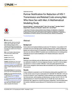
According to Equation (221, if experimental values of the frost density and temperature distribution are known, then the water vapor mass flux can be calculated as a function of the "x" variable as shown in Figure 1 within the frost layer. Observations by several authors (References 1, 2, 3, 13, and 14) indicate that the frost density is nearly spatially invariant in the "x" direction. This means the total water mass flux, fit, consisting of water vapor and nucleated water drops, is given approximately by, .

tit -= dx

.

.

mt =“exp X

x

,

S

where in is the experimentally calculated value of the water f=w mass flux into the frost surface from the surrounding air and X is the frost thickness. If one observes that in, 1. md for all S values of x, then no nucleated drops have formed: this means a. supersaturated state is unlikely. If one observes that . of x, then nucleation has occurred, and mt ' md for somevalues thus supersaturation might be possible. Note that homogeneous nucleation and nucleation on nucleating sites in the frost layer cannot be experimentally distinguished. Thus we cannot state definitely if supersaturation has occurred. If r?td = m, at the 2-11

.--

(24)

frost surface or at distance, xs, then we have a good method predicting the frost density growth rate for which a formula will be derived in Section 4.

for

Figure 2 shows a plot of fid and fit calculated from an experimental run of Brian, et al. (Reference 11, where the wall temperature was at 80°K. The steep rise of the md curve is due to the temperature dependent relationship of D and Pv in Equation (22) for the temperature increase from 80°K to about 265OK. In comparison to the fit curve it is probable that some supersaturation has occurred, given the magnitude of the difference between mt and rhd. At distance xs from the wall we note that fid is equal to fi t* A data set with a more reasonable temperature range applicable for frost formation on an aircraft can be obtained from Yamakawa, et al. (Reference 13). Here the range of temperature, in one specific case, is from -22OC to -3.3OC. Although the experimental temperature distribution within the frost is not available, indications are that for this small temperature range, the temperature profile can be roughly approximated as a linear function of x. Thus, the temperature gradient for Equation (22) is given by

dTz dx

Ts - Tw X

= 66.78

OK/cm

,

(25)

S

as obtained from experimental data in Reference 13; where xs = 0.28 cm. At this frost thickness the frost density is 0.1110 g/cc and the ambient absolute humidity is 0.0049 as obtained from the data. Substituting these values into Equation (22) gives the layer, fid curve shown in Figure 3. For the top half of the frost the md curve agrees closely with the I%, curve calculated from While for the lower half of the frost layer, experimental data. These observations mean that down to a wall than fi t* md is greater say the frost layer is in temperature of -22OC we can confidently at the distance xs, we find that In addition, a saturated state. Efi The conclusion is that the water vapor thermal conducmd t' tivity is valid for most frost formation situations and an accurate method for calculating the water mass flux entering the frost surface has been obtained. 2-12

Now kv can be compared directly with ka and ki for From Reference 10, with the same an order of magnitude analysis. data used in evaluating the radiation effective conductivity, with equation (231, we obtain at the frost surface, kV

= 0.0111

w/m°C

.

(26)

conductivity But since ka = 0.0236 w/mOC, the 'water vapor thermal At higher frost density, cannotbe ignored at low frost density. actually decreases due to the porosity term in Equation (23) kV the At close to ice density the term ki = 2.37 w/mOC indicates the order of magnitude So far; dominating influence of ke. calculations show that particular attention must be devoted to developing the air-ice thermal conductivity which would include a complicated frost structure modeling and perhaps also the water vapor thermal conductivity at low fro.st density. 2.1.4

Forced-Air

Enthalpy

Rate Term,

G -Cp $

to determine, The air mass flux, Ga, is difficult because it is strongly dependent on the frost structure. If the frost structure consists primarily of ice cylinders that penetrate deeply into the ambient flow of air, then perhaps Ga can be approximated conservatively to the upper limit, e.g., But that situation is unlikely since, as shown above, frost That is, the initial the frost structure is not simple. may form ice trees, but the frost thickness is so thin that it This means the barely penetrates the momentum boundary layer. of the free stream velocity. velocity, va, is some small fraction the frost density will also increase, As the frost thickens, This frost structure causing a"close knit mesh of ice dendrites. It is would eliminate any forced-air flow through the frost. noted the wall is impermeable,s-o there is no suction or blowing In the study of heat and mass underneath the frost layer. transfer coefficients in Section 3, for the forced convection frost surface area for the case, we show that the effective turbulent heat transfer coefficient remains a constant for all But for the laminar, values of the frost density and thickness. PaL

l

2-13

l

natural convection case, there is no frost the heat transfer coefficient. Thus it is momentum boundary layer begins at the frost laminar natural convection case and begins minute distance below the frost surface in forced convection case. In this situation, within the frost layer is the total water set equal to Ga.

surface effect on concluded that the surface for the at some constant the turbulent the only mass flux flux, in,, which is

Consequently from Brian data, as also used to evaluate kv and k,, a high estimate is made of the forced-air enthalpy rate term in Equation (7) for comparison with the hd term by using the measured temperature gradient for the water vapor mass flux at the frost surface. The result is, . dT mdsCa dx I S

heat

This contribution

X 1O-4 w/cc.

can be compared to a low estimate calculated by setting md, x- S

SC dx in Equation

8.44

=

(27)

of

the

latent

(28)

(74 to get . mdSLS X

=

2.91

x 1o-2 w/cc*

(29)

S

Comparable results were also obtained within the Therefore the heat transfer rate by the forcedfrost layer. air enthalpy rate is much lower than the latent heat release In fact it also appears that the rate within the frost layer. heat transfer by radiation within the frost layer is of the same order of magnitude as the heat transfer by an enthalpy change Since the experimental data is not due to the water vapor flux. accurate to four significant digits as would be required both by the forced-air enthalpy rate and the radiation heat rate, the

2-14

terms for the rate are only

conductive heat rate retained in Equation d dx

[

keE

dT

1

and the latent heat (7) The result is

dfid dx

=-L

release

.

(30)

An expression for a frost thermal conductivity be derived if Equation (23) is used and substituted in the equation and integrated. Thus, dT Kz=qo i with

K = ke + k,

,

-

where q. is a constant heat flux at the wall and K is conductivity of frost. With the simplified equations all other approaches obtained from the literature for the frost thermal conductivity can be explained. 2.2

can above

(32)

the thermal above, calculating

APPROACHES FOR CALCULATING K 2.2.1

Brian,

et al.

Approach

If the heat flux and the temperature gradient are measured, as wasdone in the frost experiments by Shah (Reference thermal conductivity and Brian, et al. (Reference 11, a frost It is can be calculated easily from the above equations. important that the heat flux should be measured at the wall as is done by Shah (Reference 2) as well as by Brian, et al. (Reference 1) rather than at the frost surface. The reason is because, due to the latent heat contribution, the heat flux becomes 'lower at the frost surface than at the wall. Some empirical expressions for the thermal conductivity of frost, based on the experimental data by Shah (Reference 2), Brazinsky (Reference 15), and Brian, et al. 10) in by Brian, et al. ( Reference (Reference 1), as developed SI units are

2-15

I

-

(31)

2)

K1

= 2.405

where K2

pf

= 3.595

where

Pf

K3 =1.564x10 where

x 1O-5 T1'272 < 0.025

g/cc

T5=44 + 2.042

> 0.025

g/cc

Pf ' 0.025

g/cc

(33)

and T < 255O K;

x lo-l5

-5 T 1*441

x 10 -5 p f T1.74

+ 3.931

x 10 -12(~f-0.625)T4=84,

and T > 255O K; + 4.252

(34)

and

x 10-8(Pf-0.025)T

3.055

I

(35)

and T < 255OOK and

of the frost. where Pf stands for the average density It may be noted that this empirically developed thermal conductivity is a linear function of the frost density. Later on it will be shown that this relationship is valid only within the experimental range of frost density up to 0.13 g/cc. Serious problems are encountered if one attempts to use the above type expression for thermal conductivity with other This is because a number of factors such as the thermal data. conductivities of water vapor, air, ice, and the frost structures, which play important parts in the expression for the thermal conductivity of the frost, have not been considered in the above model. 2.2.2

White's

Approach

Another approach to determine the frost thermal conductivity developed by White (Reference 4 ) using the empirical relations to fit the Shah data (Reference 2) where kv Of Equation 32 is given by kv =

Deff Ls.2pv , and R 2T3

(36)

V

ke

= (0.1684

+ 35.39

pf/pwater)

X (-0.01356

and 2-16

+ O.O001579T),

(37)

Although this approach is more where D = 100 mm2/sec. eff theoretical than that of Brian, et al., since it takes into account more variables, it is still hampered by the fact that k, and ke are treated Another problem is that as empirical terms. this approach is valid only in the experimental range of Shah's data (Reference 2) which is PfL 0.13 g/cc. 2.2.3

Biguria

portion of that if the air thermal The effective relation k effair

and Wenzel's

Approach

Since the water vapor diffusion occurs only in the air the frost, Biguria and Wenzel (Reference 3 ) suggest effective air thermal conductivity instead of the true results. conductivity is used, one can expect better air thermal conductivity can be obtained from the

=lca+p;~pv(~)(&-j

=ka+q

(38)

which is based on Equation (21) of Reference 3 and Equation (23). It may be noted that for obtaining the air effective conductivity, the tortuosity and the porosity expressions in the vapor effective conductivity are neglected as they have no use as corrections in According to Biguria and Wenzel the air portion of the frost. (Reference 3) one can obtain a better expression for ke by using For frost (10) to (16). k eff air instead of ka in Equations and Wenzel claimed that densities greater than 0.05 g/cc, Biguria a good fit to their experimental data was obtained by using this The experimental thermal approach and Equations (15) or (16). conductivity of frost was obtained, however, by measuring the heat the thickness of the frost, and the wall and flux at the wall, In order to apply the theoretical frost surface temperatures. thermal conductivity equations to the data, Biguria and Wenzel implicitly assumed the frost layer has uniform temperature,

2-17

These assumptions require and density distributions. structural, the wall temperature to be a high temperature at around 250° K, the frost to be formed in a specified structure, and the ambient absolute humidity to be in a specified range near saturation(Reference 1) and the data of Brian, et al. In contrast, 2) typically has the wall temperature at 80° K, Shah (Reference more spherical ice formations than ice trees, and an ambient Thus it absolute humidity at a fraction of the saturation level. iS expected the approach by Biguria and Wenzel will not fit (Reference 1) and satisfactorily to the data of Brian, et al. Shah (Reference 2). This actually turned out to be the case. The basic disadvantage in this approach is the requirement of a. uniform temperature and structural distribution of the frost. 2.2.4

Jones

and Parker's

Approach

density is spatially By assuming that the frost is the invariant so that the amount of water vapor being frozen the change in the vapor layer, same at all locations in the frost mass flux with distance is dind -= dx

(28)

.

by the temperature where mds is the water vapor flux driven gradient at the frost surface. Jones and Parker (Reference 5) have used this relationship to model the heat transfer mechanism in the frost layer, and thus also the model of the frost thermal Substituting the above expression into Equation (30) conductivity. and integrating, we get, 'd, -LS ke + = (39) x+qo I X S

where

90

hB hm Ta TS

wa ws

(w/m*) , = hH (Ta - Ts) + hmLs (ua - us) is the heat transfer coefficient (w/m* "C), is the mass transfer coefficient (g/m* secOC), is the ambient air temperature (OK), is the frost surface temperature (OK), is the absolute ambient humidity, and is the frost surface humidity. 2-18

It

may be noted here, ke, which is computed in the usual way as in Equations (10) to (16), does not contain the expression for keff air. Also, Jones and Parker (Reference 5) used the incorrect expression for ke by using Brian, et al.'s (Reference 1) empirical frost thermal conductivity. This If a linear vapor mass flux with approach has two difficulties. distance which releases the latent heat is assumed, then, because of what has been shown in Figures 2 and 3, a supersaturated state would have to exist in Brian, et al. 's data (Reference 1) and a subsaturated state would have to exist in Yamakawa's data (Reference 13) within the frost layer. This dual state is physically unlikely, especially if several ice crystals also exist The second along side of the moist air within the frost layer. difficulty is that this approach cannot be compared with experican be calculated from each data mental data unless the term fi dS set. Usually the values of rhd are absent in the literature S available. 2.2.5

Summary of the

Four Approaches

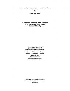
If one examines carefully the aforementioned approaches which have been established on the basis of a controlled environment, one will find that they are not satisfactory for the aircraft frost formation problem where the environmental variables have different ranges. The validity of the first approach, given by Brian, et al. (Reference l), is restricted to frost densities less than 0.13 g/cc and very low wall temperatures and ambient humidities, as indicated in Table 1. If the empirical frost thermal conductivities based on ice density are extrapolated, the sharp disagreement with the actual thermal conductivity of ice is apparent in Figure 4. Similarly, if the same is done on the the resulting curves in Figure 5 show basis of air density, the disagreement with the actual thermal conductivity of the air. It may be noted that the effective conductivity of water vapor, which becomes negligible for temperatures less than 225' K in the due to the rapid decrease in D and PV' was not considered On the basis of the same arguments, thermal conductivity of air. 2-19

TABLE I Summary of Approaches to Calculating Frost Thermal Conductivity

Range of Application

Approach Brian, et al. (Reference 11

White (Reference

4)

Pf 2 .13g/cc

Jones & Parker (Reference UDRI Approach

Limitations Average Thermal conductivit y will fit data at other temperatures.

TW

Pf’

Semi-empirical

= 800 K

.owcc~Pf-ice 3)

Modeling of the Frost Structure

Empirical

=W

Biguria 6 Wengel (Reference

Modeling Technique

Simple Frost structures is postulated

Semi-empirical

Vapor diffusion frost layer is postulated

Mostly partly

Complicated frost structure is postulated for vapor diffusion, geometrical shapes of ice dendrites, and for frost aging.

5) 'a< 'f' 'ice 8Oo KcTw250° K .13g/cc

Vapor diffusion in frost layer postulated

theoretical empirical

in

not wall

Same as Brian, (Reference 1)

et al.

Same as Brian, (Reference 1)

et al.

Super saturation within frost layers is unlikely.

150

200

Temperature

Figure

4:

Thermal

conductivity

versus

250

OK

temperature

at ice density

300

0.03

/ / /

b; ” 0.01

/

'K2

/ / /

0 .O(

100

50

Temperature Figure

5:

Thermal

conductivity

250

200

150

versus

OK temperature

at air

density

the approach given by White (Reference 4) is found unsatisfactory for our problem. Since the state of super- or subsaturation within the frost layer is unlikely to exist, Jones and Parker's approach (Reference 5) is not being used in our analysis. When the available experimental data could not be fitted to the theoretical approach suggested by Biguria and Wenzel (Reference 3), an attempt was made to see if the experimental values of frost thermal conductivity given by Brian, et al. (Reference 1) could lie between the curves represented respectively by Equations (13) and (14) for either spherical air pores or spherical ice particles. The encouraging results in Figure 6 showed that the frost thermal conductivity is a linear function of porosity or frost density for porosities greater than 0.85. This gave a motivation to propose a new model, based on Biguria and Wenzel's theoretical approach (Reference 3), but which includes frost structure parameters which could be empirically derived to fit Brian, et al.'s data (Reference l), as well as other data. 2.2.6

The UDRI Approach

The proposed model makes the following assumptions about the frost structure as shown in Figure 7. At low frost density, or at high porosity, two types of frost structure predominate. One is the ice cylinders created by the internal diffusion of water onto the ice, which result in a parallel conductive heat transfer. The other portion is the ice spheres created by nucleation of water vapor, resulting in a much lower conductive heat transfer. The total structure of the frost is then the random mixture of ice cylinders and ice spheres (Figure 7a). At,high frost density, or low porosities, completely different dual structures begin to take shape. In contrast to the low density case, spherical air voids are formed in place of ice cylinders (Figure 7b). This results in enhanced thermal conduction. Also, in place of the ice spheres, stratified layers are formed. The total frost structure is then a random mixture of air bubbles and ice layers.

2-23

3

2

Continuous

1

Continuous

air

ice

phase

phase

Experimental 0 0

0.25

0.50

0.75

1.00

Porosity Figure

6:

Thermal conductivity versus porosity at 211 OX 2-24

frost

:

:

$u

Random mixture at high porosities

B

1;:

:

:

Frost

of ice cylinders and ice or low frost densities

Layer

spheres

(a)

X

X

s

-

I

lo 0 0:

I I I

0 0 0; ---1 000 -f -1

000

-:

I I I I

Frost

4

0 IIO l

I

Random mixture at low porosities

of ice planes or high frost

and air densitkes

-Y bubbles

(b)

Figure

7.

Frost

Stucture

Model of

2-25

the

present

work

Layer

With such a model of the frost structure, the equations for air-ice thermal conductivity presented earlier are combined in two ways. First, an attempt was made to arrive at the upper limit and the lower limit of thermal conductivity as a function of porosity. The second part attempts to ascertain the combined contribution of the upper limit and the lower limit of the thermal conductivity to the frost thermal conductivity as a function of temperature. Noting that the thermal conductivities for ice cylinders and for air bubbles are close to each other for all porosities, a simple interpolation rule is used to obtain the upper limit of the thermal conductivity. kU

kb kC

= (1-B)

kb + ,9kc (upper

= ki. [l

- 26 (:

= (1 - f3)ki

5 :)I/

+ f3keff

limit) [l

air

I

+ B(: (ice

(40) i E)](air

bubbles),

cylinders),

(11)

c% = k eff air'ki . ' Likewise, the lower limit of thermal conductivity formed by an interpolation between thermal conductivities for ice spheres and ice planes. kl

= (1 - B)kp + Bk

ks

= ki

(lower

limit)

- 1) kl

+ (30c - 1) kU)2

+ (30c - 1) kU +

+ 8klku]

2-26

L'2)

is

(41)

3 + 2B(a - ' 1)] / [3 - B (* a ')](ice spheres), C k. k eff air k (ice planes). p = (1 _ & + kiB eff air To determine the combined contribution of the upper and the lower limits of the thermal conductivity to the frost thermal conductivity, the random mixture model of Brailsford The present and Major given by Equation (15) is utilized. model of thermal conductivity of frost given as K = 1/4{((38,

(13)

K

(36 C - 1) kl

(14) (10)

(42)

The proportion of the is used to combine k,., ,kU, and@ c. ice spheres and ice planes given volume, Bc, representing parabolic function of the porosity B is 2 , =a+bB+cB

frost as a (43)

BC

or functions of temperature. where a, b, and c can be constant of the frost volume representing ice cylinders The other portion and air bubbles is given by (44) It is plausible to assume the frost takes on a completely spherical air voids structure when the porosity in the frost approaches zero or the density of the frost approaches that of/ice. This assumption when translated into boundary condition for"Equation (43) , gives Bc = 0 for B = 0 and thereby 'a' is found to be zero. Another plausible assumption is that all frost structures converge to the same structure as the porosity It gives approaches zero regardless of the frost temperature. then be a strong function of 'b' as a constant and 'c' will Since each curve in Figure 8 is at a different temperature. temperature, it is possible to determine the values of 'b' and ‘C’ from it. The result indicates that 'b' is indeed a constant and 'c' is a function of local temperature of the frost, hence the value of Bc becomes 2 (45) . %

of 0.99 as a fit compare model, ductivity denoted

correlation As shown in Figure 8, it gives a multiple and a standard deviation to the third decimal place In order to to Brian, et al.'s data (Reference 1). as predicted from the proposed the frost conductivity, thermal conto other experimental data, an average frost The average frost thermal conductivity, is needed. as by z, is defined I g=

TS

TW

K dT

Ts - Tw 2-27

(46)

r

0.20

X

0.18

T=267OK x

isi 0.16

"E

/

2

T=25S°K

54" 0.14

2

V

d 0.10 2 $ E

l-l 3 B

T=211°K

x 0 A

0.08

/

T=17S°K 0.06

T=136'K

0.04

0.02

0.0

/

0.05

0.07

0.09

Frost Figure

8.

0.11 Density,

L 0.G pf(g/cc)

0.15

0.17

Comparison of the Present Frost Thermal Conductivity Model with Experimental Data of Brian, et al. (Reference 1)

2-28

where Ts is the frost surface temperature and Tw is the wall temperature. The calculated value of ii agreed excellently with Brian, et al. 's data (Reference 1). But Yamakawa, et al. (Reference 13) and Nakamura's data (Reference 14) gave biased values on the low side for x. The reasons for the discrepancy seem to be the following. The effects of frost aging and the size of the water droplets arriving at the frost surface cause the formation of various types of frost structures. In Brian, et al. data (Reference l), where (47) TW = 80° K and (Pa = 20%, the extremely low temperature coupled with low relative humidities is found to cause the formation of several large size water droplets, which may freeze instantaneously on the wall. This conclusion was derived from Rosner and Epstein (Reference 11) in the case of fog formation near cold surfaces. As the frost surface temperature increases with time, the smaller water droplets arrive at the frost surface and due to sharp temperature gradient, nucleation density takes place within the frost layer. Also, as the frost These effects increases, the ice dendrites begin to mesh together. are due to the aging of the frost and are aptly included in the empirical relationship for 8,. On the other hand, in Yamakawa, et al. (Reference 13) and Nakamura (Reference 14) data where TW = 245O K and $a = 40% to 90%, the much higher wall ‘temperature coupled with higher ambient humidities are expected to cause the formation of smaller water droplets which would not freeze instantaneously on the wall. Therefore, initially, the value of 8, for their data should be lower than that of Brian, et al. data (Reference l), as the presence of the spherical ice particles in the frost layer is less probable. In this case, the water droplets tend to remain at the same size and due to the higher wall temperature, nucleation within the even though the frost surface temperafrost layer is not probable, Due to the foregoing reasoning, it is ture increases with time. apparent that the expression for B, should also include 2-29

the effect of wall temperature and the effect of the aging On the basis of the reasons given above, and for frost. preliminary studies on frost formation, the expression for proposed as 2 2 = .l+ 8o -T BC’ B (.526Tw + 315)2

1B}

of 13, is (48)

When the proposed Equation (48) is used for qalculating the average thermal conductivity of the frost at Tw around 250°K, the results show a good agreement with the data 13) and Nakamura (Reference 14). by Yamakawa, et al. (Reference It may also be noted that at Tw = 80°K, Equation (48) reduces to Equation (45) which gives excellent agreement for the data Thus the expression for thermal by Brian, et al. (Reference 1). conductivity with 6, given by Equation (48) is used for the present frost formation model and the results are discussed in the last section of this report.

2-30

SECTION 3 HEAT AND MASS TRANSFER COEFFICIENTS The diffusion of water vapor from the moist air across the frost surface and then into the interior of the frost layer is the mechanism by which the frost layer grows. The rate of growth will be determined by the rate of this mass transfer and the rate of heat transfer to and from the frost layer. To quantitatively predict the growth of the frost, the rates of mass and heat transfer across the frost surface plane shown in Figure 1, must be determined. As in other heat and mass transfer problems it is convenient to represent these convective transfer rates as a heat or mass transfer coefficient multiplied by a suitable potential difference, either temperature, T, or concentration, w, as appropriate. That is, q, = hH(Ta-T,), and This section deals with the several methods of fit = hm(wa-ws& representing the heat and mass transfer coefficients that have appeared in the literature6 These coefficients are analyzed and compared with the experimental data available. The poor comparisons obtained indicated that modified coefficients were needed and consequently are developed in this section. Because of the limited availability of data;the heat and mass transfer coefficients could only be compared at two extreme experimental conditions. The first condition is the frost formation on a vertical wall under laminar natural convection. The other condition is the frost formation in a horizontal duct under turbulent forced convection. Therefore, only the heat and mass transfer coefficients for these conditions are examined. Heat and mass transfer processes for other conditions, such as the airfoil geometry, are not examined because no experimental data is available for comparison. By analyzing for the two extreme experimental conditions two tasks can be accomplished. The first is that the heat and mass transfer processes for the other conditions can be inferred, and secondly, the frost formation model can be severely tested for accuracy under the extreme conditions. 3-l

I

-

Because accurate transfer coefficients for the frost structure are not available in the literature some investigators have tried to use empirical correlations such as are used in other convective heat transfer problems. Two of these for turbulent forced convection in a duct are the Colburn equation (Reference 16), StPr213 or

= 0.023 Re0.8

Nu = 0.023

Remoo2 Pr1'3

= hHL/ka,

for where Nu, Pr, Re and St stand respectively Reynolds and Stanton number, Nusselt, Prandtl, Boelter equation (Reference 16) Nu = 0.023

Reoa8Proo4

Once the heat transfer coefficient available to find the mass transfer convection (Reference 6), hH/hm

and the

where

Chilton

= c;

- Colburn

the non-dimension and the Dittus -

.

(50)

is known, some methods are coefficients under forced

(51)

I

analogy

(49)

(Reference

6)

-2/3 I hH'hm = CPLe heat of air (J/g OK), Cp is specific hH is heat transfer coefficient (w/m2 "Cl , * hm is mass transfer coefficient-(g/mLs), and Le is Lewis number = PaCpD/ka .

(52)

These relationships have been slightly modified for special Kays and Perkins (Reference 16) show that for the situations. Prandtl number between 0.5 and 1.0 and a constant wall temperature, the heat transfer coefficient for turbulent forced convection in a duct can be better correlated by the equation Nu = 0.021

Reoa8Proo6

,

(53)

3-2

1

than by the Colburn equation. For a vertical plate under natural convedtion, the Nusselt number, Nu Z’ is correlated local Grashof number, GrZ by the equation (Reference 6) N”Z

= 0.421

GrZ l/4

Pr 1'2

laminar to the

.

(54)

To show that these transfer coefficients need modification, the heat transfer coefficient experimentally obtained by Yamakawa, et al. (Reference 13) and Nakamura (Reference 14) were compared with Equations (53) and (54), respectively. Equation (53) when compared to Yamakawa data gave errors biased by about 200%, while Equation (54) compared to Nakamura data gave about-a 25% error bias. Further significance of these errors will also be shown in the next section. Other experimentors (References 1, 2 and 4) have attempted to measure the accuracy of the heat and mass transfer processes for frost. they have not succeeded for Unfortunately, all the possible experimental ranges in correlating the experimental data by empirical relations. To explain the experimental disagreements noted earlier and the difficulties of several experimenters, three postulates are advanced. The first is that the suction or blowing of the water vapor at the frost surface will affect the thermal boundary layer Secondly, fog forand thus also the heat transfer coefficient. mation or nucleation in the boundary layer will enhance the water vapor mass transfer and possibly also enhance the heat transfer. due to frost porosity, the heat and mass transfer coLastly, efficients are affected by the effective area of the frost surface With these which equivalently can be termed as frost roughness. of Nakamura (Reference 14) three postulates in hand, the results to determine and Yamakawa, et al. (Reference 13), are analyzed which of the postulates are significant for a particular experimental condition. Thus the modification of the heat and mass transfer coefficients can be quantitatively described for the two extreme experimental conditions and qualitatively described With the modified cofor all other experimental conditions. to the frost surface efficients in hand, the heat and mass fluxes can be calculated. 3-3

3.1

LAMINAR NATURAL CONVFCTION

The results from Nakamura (Reference 14) show that in laminar natural convection on vertical plates the surface roughness has no effect on the heat transfer coefficient because the sensible heat flux from the air.to frost is mostly conductive, rather the nucleation in the boundary layer has Also, than convective. only a small effect on the heat and mass transfer coefficients, because the amount of vapor mass flux is usually so small that there for natural convection, the However, is only minute fog formation. mechanisms- are coupled together momentum, heat and mass transfer The analysis for this problem is taken from in the boundary layer. Okino and Tajima (Reference 17) for a vertical plate under laminar After correcting an algebraic error* in their natural convection. analysis, the results a;eHas follows. hmH H (551, = n(l+os) = n/c I ShH= p D N"if k a a where l/4 n = - 38 (57) + SC@ ) I

gH3

GrH =

c=J Q =

+

v2

I Wa-Ws I 1. 6453 + 2.6453~~1

,

1

(58)

cp +1-Q

a2+2g

(59)

1 + wa (60)

1 - us is g is H is ws is SC is

V

equations

kinematic viscosity, gravitational acceleration height of plate (m), saturated absolute humidity, Schmidt number.

The Nusselt and Sherwood numbers fitted Nakamura's data (Reference

*The algebraic error denominator instead

(m/s'), and (NuH and ShH) by these 14) quite well.

is that the term & in n was placed in of the numerator of equation (57) above. 3-4

the

(56)

3.2

TURBULENT FORCED CONVECTION

In the case of forced convection however, the mass transfer has only a minor effect on the heat transfer coefficient. This is shown as follows. A conservative estimate of the blowing parameter based on Yamakawa, et al. data (Reference 13) gives . F = mt = .00002 (61) 'a 'a which, according to a graph presented by Rohsenow and Hartnett (Reference 6), is so small that the exponent of the Reynolds number in Equation (53) remains constant at 0.8. A cursory look at Yamakawa's Nusselt number (Reference 13) versus Reynolds' number plot in Figure 9 verifies this conclusion, which is in opposition to a conclusion drawn by Yamakawa, that the mass transfer affects the heat transfer coefficient. Yamakawa, et al. (Reference 13) thought that the mass transfer could be eliminated by making the inlet humidity the same as that at the frost surface and to establish their conclusion, they took the convective heat as the only heat source at.the frost surface. The heat fiux, however, as measured at the wall below the frost layer, is due to the temperature greater than the convective heat because, gradient driving force, the latent heat is also being released in the frost layer. There is no evidence that any correction was made for the latent heat contribution and thus, an incorrect Yamakawa (Reference 13), interpretation of the data was obtained. also makes the point that the water vapor nucleates ir, the This process thermal boundary layer above the frost surface. releases the latent heat and causes a change in the temperature as observed by Yamakawa, profile in the thermal boundary layer, which would change the way the heat transfer coefficient is forced related to the Reynolds' number. However, in the turbulent Re _> 104) the heat and mass transfer convection limit, (i.e., mechanisms are effectively decoupled because the sensible heat flux is much greater than the heat flux generated by the release it can be assumed Therefore, of the latent heat through freezing. that the latent heat release rate has a negligible effect on the heat transfer coefficient. 3-5

On the other hand the heat transfer coefficient is affected From our analysis of Yamakawa, by the frost surface roughness. of the effective area of et al. data (Reference 13), the ratio the frost surface to a smooth area is found to be a constant The frost roughness variety has no effect on hH because at 1.95. the boundary layer is already turbulent and hH is experimentally the usual heat Therefore, independent of the frost porosity. transfer coefficient is increased by a factor, r = 1.95, as is shown by the correlation, (62) = 0.021 Re'8 Pr' 6 with hi = hH(1.95), hHDe ka where hH = heat transfer coefficient of empirical equation and heat transfer coefficient. h?i = experimental to date A Equation (62) is believed to be the most accurate coefficient over frost and is for calculating the heat transfer forced convection. being used as the correlation for turbulent Equation (62) to There is very little scatter when applying Yamakawa's data, (Reference 13) even for points corresponding to relative humidities from 56% to 97 % as shown in Figure 9. Furthermore, the points corresponding to the different humidities This supports the assumption that the show no preferred bias. nucleation in the boundary layer has a negligible effect on the heat transfer coefficient in this experimental data. Nu =

The mass transfer coefficient could be obtained from heat transfer coefficient using the Chilton - Colburn analogy (RefHowever, Yamakawa's data (Reference 13) shows a erence 6). strong scatter for the analogy of the heat and mass transfer. It is difficult to determine what causes the scatter of the hfi vs hi (experimental mass transfer coefficient) plot shown in are not identified by the corresFigure 10, because the points trends can be ponding humidities and Reynolds number, yet certain perceived. For a mass transfer coefficient less than about 30 as if from the g/m2s I where hm = hi, hi can be calculated Chilton - Colburn analogy shown as the upper line in Figure 10,

3-6

100 0 ambient

1 800L

500I-I

relative

humidity

0 97% A 70% D 56%

,

Experimental

200

30 20.

10 x10- 3x10'4 Figure

5

6

78 91x10' i Reynolds Number, Re between Nusselt's 9. Relationship number (Reference 13)

3

4

7. 8 9 1X10=

number and Reynolds'

Correlation

0.0

h* 2:

12.5

(g/m*s) 37.5

50

62.5

75

80 80

0.c 100 h; Figure

10.

150 (kg/m2*hr)

200

250

Relationship between local heat and mass transfer coefficient (Reference 13)

300

h;/l-

=

h

h; This correlation roughness on the But this correlation the mass transfer roughness in the

/he

H

-2/3 m = Cp Le

.

(63)

seems to rule out the effect of the surface experimental mass transfer coefficient, hi. is tentative because in the turbulent flow coefficient should be affected by the surface same way as the heat transfer coefficient is.

At h; = 30 g/mLs one can see a very strong scatter in the data, and it is biased in such a way that one can propose a mass flux enhancement due to nucleation in the thermal boundary layer. By using Epstein and Rosner's approach (Reference 111, it can be shown that for the wide range of wall temperatures and ambient humidities, the water vapor mass flux increases by a factor from 1.0 to a maximum of 2.95 over the usual mass flux of condensation That is, on the wall surface. 1 < h;/hm

the

.

(64)

For the mass transfer coefficient Chilton - Colburn analogy between hfi/h&

shown as the lower enhancement factor Coiburn analogy is turbulent flow. 3.3

f 2.95

= 1.5

Cp Le -2/3

greater than 45 g/m2s, h,$ and h$ can be modified

I

line in Figure 10, which means that the That is, if the Chilton is hz/hm = 1.3. still valid for a rough surface and a

to

(65)

-

SUMMARYOF HEAT AND MASS TRANSFER COEFFICIENT EQUATIONS

So far we have considered the extremes of the experimental data. At one extreme we have the laminar natural convection, and at the other extreme we have the turbulent forced convection. In the region of combined natural and forced convection not only the heat and mass transfer are coupled but also the nucleation in

3-9

-- _. _._._-. ..-. ._

-.- .

-.

___-

.._.

the boundary layer and the frost surface area affect the heat transfer to a.significant degree. The surface roughness will affect the heat transfer in two ways. The first is that the surface roughness will cause the transition point (located between laminar and turbulent zones) to occur closer to the leading edge. Secondly, in the laminar zone, the effective surface area for the heat transfer coefficient is unity relative to the smooth surface area, but the effective area is 1.95 times greater than the smooth surface area in the fully turbulent zone. Although the effects of nucleation in the thermal boundary layer upon the heat transfer was considered negligible in both extreme experimental data, it may become significant in the combined natural and forced convection when the latent heat release rate in the boundary layer may become the same order of magnitude as the sensible heat. from our studies of the Lastly, data, the perturbations in the mass transfer coefficients is caused by the fog formation or nucleation in the boundary layer and by the frost surface roughness. The maximum enhancement in the mass transfer coefficient appears to be at the ratio, hz/hm=1.3. For the comparison of the frost formation model to experimental data, Equations (55) to (60), (62) and (65) will be used The frost formation model however, can be immediately tentatively. generalized to other air flow geometry, and surface roughness conditions, if the heat and mass transfer coefficients can be To obtain the transfer coeffiobtained for these conditions. cients for an arbitrary airfoil geometry, computer programs need to be developed to couple the boundary layer models with the There are such programs in the literature potential flow models. (References 18, and 19) but none has yet satisfied our requirements to include the effect of water vapor mass flux nucleation and Some surface roughness on the flow properties near the wall. ways of calculating literature (References 20, and 21) provides the influence of surface roughness and the water vapor mass flux Other literature (References 22 on the transfer coefficients. and 23) provide ways of calculating the enhancement of the

3-10

mass transfer coefficient due to nucleation in the boundary layer. Only a small amount of literature is available for analyzing the heat and mass transfer problem for combined natural and forced convection. A synthesis of this literature will be required for the study of overnight frost formation on an aircraft.

3-11

SECTION 4 THE SIMULATION OF FROST FORMATION 4.1

FROST FORMATION MODEL

thermal conductivity was formulated In Section 2, the frost so that the heat flux through the frost layer could be calculated. coefficients were In Section 3, the heat and mass transfer formulated so that the heat flux to the frost surface from the By matching the two heat fluxes at the air could be calculated. frost surface the temperature of the-frost surface can be calculated. The frost surface temperature will change with time because the frost layer is becoming denser and thicker, which in turn affects During the the computations of the heat flux in the frost layer. process of frost formation it is assumed that the part of the water vapor transported to the surface freezes at the surface so The remaining water as to increase the thickness of the frost. vapor is diffused into the existing frost layer before it freezes. Since the frost density is'assumed to be spatially invariant in a the water vapor diffusion flux direction normal to the plate, entering the frost surface from the surrounding air is given by *ds

=

at

xs

(66)

'

mass flux where rhds' Pf and xs stand for water vapor diffusion frost density and frost thickness respectively. the surface, obey the diffusion fid will Also, the water vapor mass flux, Equation (18) and will be driven by the temperature gradient throughout the frost layer. The water md

frost

Equation surface

diffusion

flux

is

(;;2)[zT

given

by Equation

(22) (67)

-

‘)

+$

l

(67) can be evaluated at the frost surface gradient temperature Ts, the temperature

4-l

if dT dx

the I /

at

Combining Equations and the frost thickness x are known. (67) allows th'e frost denzity to be solved for as a function time. To obtain a value for steady-state heat equation This is, the equation K with K given conditions

by Equation

frost surface for the frost

dT dx

(66) and of

temperature, Ts, the quasilayer is to be solved.

= q,

(42)

is

(68)

to be solved

T = Ts at x = xs

and

with

the

T=Twat

boundary x=01

where = hH

g0

(T~-T~)

+ hmLs(Pa

- P,,)/P,

(69)

+ ECJ (Ta4 - Ts4)* This

gives TS s

KdT

=

xsqo

(70)

l

TW

The temperature gradient at the 90 -= dT dx I s K(Ts) '

frost

surface

The thickness of the frost can be computed related of the frost (P, xs ) which is directly coefficient and the water vapor density by

Since these equations cannot be solved analytically, niques are used to solve these equations to obtain and the density of the frost.

4-2

is

given

by (71)

from the weight to the mass transfer

numerical techthe thickness

4.2

THE NUMERICAL SCHEME FOR FROST FORMATION MODEL

The scheme begins by assuming a small initial value of frost The initial frost density thickness, xso. density, pfo and frost + ~~1 and is set equal to that of the ambient air, i.e., PfO = p,(l the initial thickness is calculated by xso = h;

(ua - ww) (A to)hfo

(73)

r

where ww is the absolute humidity at wall temperature and At, is set at one second. The frost surface temperature, Ts is obtained from the monotonic nonlinear equatioh, TS

Kd=

x

rF

.S

hH(Ta-Ts)

+ hmLs(Wa-us)

+ sc(Ta4-

Ts4).

.

I

(74)

In order to solve this equation in an accurate and efficient manner, the frost thermal conductivity given by Equation (42) is first interpolated by a parabolic function in a temperature range AT and integrated to get the first term in Equation (741, (i.e., AT is (74) is solved often greater than Ts - Tw). Then T, in Equation for by an interval-halving-iterative technique so that the left term of Equation (74) is equal to the right terms. In this way successive evaluations of the complicated thermal conductivity expression (i.e., Equation (42) ) and numerical integrations can be completely avoided when iterating to get Ts. The temperature gradient at the frost surface is obtained by TS 1 K dT dT TW = (75) . -I K(Ts)

The value for the frost by using the equation,

density

ks

is predicted

for

LS

apf at

RvTs

4-3

a later

time

tn+l

I

.

S

c (76)

which is solved by using a second order Runge Kutta !'initial" "takeover" scheme, and by a second order predictor-corrector scheme. Finally, the value for the frost thickness is predicted for the same time.as the frost density, (i.e., at tn+l) by the equation, PfXs

=

m

(wa-ws)dt

+

PfOxsO

t

where the rectangular rule is used for the integration, in acknowledgement of the fact that hm and us are slowly changing functions of time. At the'same particular time, tn+l, a new frost surface temperature is calculated by returning back to Equation (74) incrementing n, and using the new values of frost density pf and thickness x S’

4-4

(77)

SECTION 5 COMPARISON OF THE MODEL WITH THE AVAILABLE EXPERIMENTAL DATA In this section, three separate classes of experimental data which are considered to be complete and the transfer coefficients considered to be well known are described and compared with results predicted by the frost formation model. The first set of experimental data that the model predicts quite accurately is that of Brian, et al. (Reference 1). Since the typical Reynolds number is greater than 10,000 and the boundary layer is turbulent in the duct in which their experiment was conducted, the correlation for the forced convection mentioned earlier by Equations (62) and (65) for the heat and mass transfer coefficients is used here. The roughness factor, r, is set at 1.95)and the enhancement factor is set at 1.3. It may be noted that these coefficients are based on the experimental data of Yamakawa, et al. (Reference 13). Table II lists the input data (Reference 1) for the frost formation model and from Brian et al. also the symbols identifying the experimental data in the next three figures. Results from the model have been compared with the experimental data giving the frost weight, density, and thickness as functions of time under different experimental conditions. The results are given in Figures 11, 12 and 13 where the computer generated solid curves are plotted along with the experimental data. The figures show excellent agreement. When the standard correlations given by Equations (49) and (52) instead of the modified Equations (62) and (65) are used in this set of data, the corresponding results are shown by the dashed curves. The comparison of the solid and the dashed curves based on the same experimental data shows that poor correlations are obtained for standard heat and mass transfer coefficients. The second Yamakawa et al.

set of experimental (Reference 13) for 5-l

data examined is forced convection

that of in a duct.

TABLE II Data Input to the Frost Formation Model for With Brian et al. Data for Forced Convection

Computer Curve No.

Experimental Graph Symbol

Reynolds I Number

Relative Humidity (%I

Comparison (Reference

Wall Temperature(OK)

1)

Air Temperature

14500

26.1

79.83

297

2

A

9316

26.2

79.83

297

3

cl 0 A

5603

26.0

79.83

297

14750

20.8

79.83

297

9247

15.8

79.83

297

5625

16.2

79.83

297

4 5 6

(OK)

---data 0 A Cl 0

0.15

h CJ go.10 \ Vb u-l I w

A

hH and hm baseed on Yawakawa data (Reference 13) hH and hm based on standard correlations (Reference 6) theory 1 1 2 4 3 2 0 4 0 0 / m /'A /*' 65 / 0 3 5

2 b V-l i!

6

0.05

0.0 0

20

40

60

80

100

120

140

160

180

200

et al.

Data

Time (minutes) Figure

11.

Weight

versus

Time for

Brian

(Reference

1)

0.35-

0.30

0.25

‘;; < 20.20 h ?I In !$ 0.15 cl

hH and hm based on Yamakawa data (Reference 13) -w-m hH and'h, based on standard correlations (Reference the'ory data 1 0 2 A 3 cl 4 0 5 A 6 a

--I-

I

3n

An

Figure

10’0

120

Time

(minutes)

6ll

12.

Density

versus

140

time

for

160

180

Brian

et al.

6)

200

Data

(Reference

1)

0.8

0.7

0.6

0.5

ul I ul

E v ::a, 5 .: i3

0.4

----data 0 n cl 0 A

0.3

0.2

0.1

hH and hm based on Yamakawa data (Reference 13) hH and hm based on standard correlations (Reference theory 1 2 3 4 5

n

6

0.0 0

20

40

60

80

100

120

140

160

180

200.

Time (minutes) Figure

13.

Thickness

versus

Time for Brian

et al.

Data (Reference

1)

6)

The roughness factor and the at 1.95 and 1.'3 respectively.

enhancement

factor

are

again

set

Table III provides the input data into the frost formation model and Figures 14, 15 and 16 show the results of the computer generated solid curves along with the experimental data of frost weight, density, and thickness as functions of time. The dashed lines, generated using the standard correlations again, provide inferior results compared to the modified correlations. Curves 1 to 4, in Figures 14 to 16, show a fair agreement with the experimental data. However; curve 5 shows a sharp disagreement with the data. The disagreement is probably due to the following complications. Since the relative humidity for this run is nearly lOO%, the fog starts forming before the water vapor enters into the boundary layer. This means that the enhancement factor becomes unity. Secondly, the water droplets reaching the surface are large, which in turn cause the frost structure to consist of a relatively large number of spherical ice-droplets. This alteration in the frost structure lowers the thermal conductivity to under the computed value. Third, the frost surface temperature quickly reaches the melting temperature, which causes the frost thickness to stabilize and the frost density to increase over their modeled values. 'The possibility of modifying the present model to accommodate these three factors will be considered for future work. The third set of experimental data examined is that of Nakamura, et al. (Reference 14) for natural convection on a vertical plate. The heat and mass transfer coefficients are given by Equations (55) and (56), and the thermal conductivity is the same as that used for the Yamakawa data (Reference 13). Table IV provides the input data into the frost formation model and Figures 17, lg and 19 show the results of the computer generated curves along with the experimental data of frost weight, density, and thickness. Experimental data in the 5th and 6th entries of Table IV are not available for Figures 17 and 18.

5-6

TABLE III Data Input to the Frost Formation Model for Comparison With Yamakawa, in a Duct (Reference 13) et al. Data for Forced Convection

Computer Curve No.

Experimental Graph Symbol

Air Velocity (m/s)

Relative Humidity (%) ---

1.6

56.2

251

284

5.0

56.2'

251

284

5.0

70.0

251

284

7.3

56.2

251

284

7.3

97.4

251

284

III A

0 A 0 Note: To calculate Reynolds = 20(1.7-xs)/(ll.7-xs) De

Number, cm.

I

the hydraulic

Wall Temperature

diameter

Air

('K)

is

1ITemperature

taken

as

("K)

hH and hm based on Yamakawa m-m- hH and hm based on standard theory data

0.16

(Reference

6)

/

0.14

/ /

/ /

0.12 Pi7 \& 0.10 Vb-' WI I co

2 0.08 aJ B 0.06 0.04 0.02 0.0 0

20

40

60

80

100

Time Figure

14.

Weight

120

140

160

180

200

(minutes)

versus

Time for

Yamakawa, et al.

Data

(Reference

13) '1 -

---data 0 A

0.30

hH and hm based on Yamakawa data (Reference 13) hH and hm based on standard correlations (Reference theory 0 1 2

6)

0.25

0.0 0

20

40

60

80

100

120

140

160

180

200

Time (minutes) Figure

15.

Density

versus

Time for

Yamakawa, et al.

Data

(Reference

13)

I I

0.8

----

Yamakawa data (Reference 13) hH and hm based hH and hm bas on standard correlations (Reference

6)

0.7 0.6

/

I

,

/-

0.5 0.4 0.3 0.2 0.1 0.0 0

20 Figure

40 16.

60

80

Thickness

100

120

Time (minutes) versus Time for

140

160

180

Yamakawa, et al.

200 Data (Reference

13)

TABLE Iv Data Input to the Frost Formation Model for Data for Natural Convection on Vertical

Computer Curve No.

wl

I

L

1

Experimental Graph Symbol

0

Comparison With Nakamura Plate (Reference 14)

Air Temperature

Plate Height (meters)

Ambient Relative Humidity(%)

Wall Temperature

0.085

74

262.46

301.06

(OK)

2

A

0.085

76

259.66

296.36

3

13

0.085

75

257.36

292.56

4

0.085

61

260.76

286.36

5

l A

0.040

53

256.56

291.96

6

m

0.040

38

258.76

291.66

(OX)

0.13

data 0 A 0

0.11 w-o.o9 8 \ b -0.07 2 m V-l &Los

l

theory 1 2 3 4

-20

40

0

0.03 0.01 0.0 3

60 Time

Figure

17.

Weight

80

100

120

(minutes)

verbs

Time for

Nakamura Data

(Reference

14)

0.35

data

0.30

0 A cl 0

the'dry 1 2 3 4

0

0.25 0

0.20 0

';; -c bJ 0.15 s-i .'I' m F: 0.10 ii -9 ?I k 0.05

0.0

I

0

20

I

40

I

I

60

80

I

100

I

120

I

140

Time (minutes)

Figure

18.

Density

versus

Time for

Nakamura Data

(Reference

14)

0 A 0 0

'theory 1 2 3 4

m A

6 5

data

0.80

0.70 0.60

1

/

0.50 0.40 zV 0.3c i 5 4 E

0.2( O.l( 0.0 0

20

Figure

40

19.

60

Thickness

80

100

Time

(minutes)

versus

120

Time for

140

160

180

200

Nakamura Data (Reference

14)

It is interesting to note that the curves 2, 3 and 4 in Figure 17 This show a very good agreement with the experimental data. verifies the accuracy of the mass transfer coefficient calculated However, the curves 1 and 2 in Figure 18 in this experiment. show a disagreement with the experimental data of frost density The main reason seems to be that the and thickness versus time. frost surface starts melting very early, causing the thickness to stabilize sooner and the frost density to increase over its modeled value.

5-15

SECTION 6 SUMMARYAND RECOMMENDATIONS Keeping in view the complexity of the problem and the sparse experimental data available, the results obtained to date are very encouraging. The good agreement of the proposed model with the three sets of experimental data available has encouraged us to further develop this model for use in evaluating the aerodynamic penalties on an aircraft having frost on its wings. Although the equations used in the present model for calculating the frost density as a function of time has done remarkably well for most frost formations, new equations must be developed to calculate the change in frost density due to liquid water seepage into the frost and for a non-spatially-uniform frost density. To realistically apply the frost formation model to an airfoil, additional considerations must also be given to the enthalpy rate terms for the aircraft skin and the frost, the complex black-body radiation to space, and the transfer coefficients for the various flow regimes and airfoil geometries. The formulation of the frost thermal conductivity used in the model has been placed on more theoretical grounds than in any previous the empiricism has been reduced to approaches. As a consequence, given by Equation determining a structure parameter, B,, tentatively 48, which covers nearly all the experimental data examined to date. However, the validity of the structure parameter B, needs to be verified at high frost density for the various values of wall-temperature. In summarizing, the present model for frost formation was constructed with a view towards its application to the overnight The model contains many complexities frost formation on an airfoil. To obtain an not considered by any previous investigator. improvement in the present model of frost formation would require In particular, specific more complete experimental data. experiments should be performed to improve our knowledge of the improve the frost density heat and mass transfer coefficients, 6-l

It is recommended that further development of the present frost model for utilization in the Aircraft Takeoff Simulation Program proceed along the following lines. Additional terms should be added to the heat balance equations to allow for radiation heat loss of the skin of the airfoil to space. This is the mechanism in nature that produces the rapid cooling of the airfoil, relative to the surrounding air, and results in frost formation. The resulting model could then be evaluated by comparison of computer results with experimental data. The experimental data, consisting of frost . density and thickness values, would be obtained from measurements on a flat plate exposed to the environment during atmospheric conditions conducive to frost formation. Monitoring of the atmosphere during the frost formation period would provide the input data to test the computer model versus the actual observational data. The predictive capabilities of the model could also be tested. Using meteorological predications of the overnight temperature, pressure and cloud cover profiles, the computer model would be run to determine the anticipated frost accumulation by morning. This result would then be compared with the actual accumulation to assess the frost prediction capabilities of the model. An accurate frost prediction model giving reliable estimates of frost thickness and density would provide significant benefits to the aviation community. Finally after having established the validity of the frost model it should be incorporated into an aircraft simulation program to assess aerodynamic penalties during takeoff. In addition to providing the initial frost condition at takeoff, the model would be used throughout the takeoff phase of operation to determine the frost dissipation, or further on the airfoil as the speed of the aircraft accumulation, increases.

6-2

especially with rate modeling, obtain a more refined empirical parameter, Bc.

respect to water seepage, and formulation of the structure

6-3

SECTION 7 REFERENCES 1.

Brian, P.L.T.,. Reid, R.C. and Brazinsky, I., Properties", Cryogenic Technology, Sept./Ott.

2.

Shah Y. T.,

3.

Biguria Thermal mentals,

4.

White, J., "Heat and Mass Transfer in Thick Frost Layers", Ph.D. dissertation University of Kentucky, Mechanical Engineering Department, 1973.

5.

J.D., "Frost Formation Jones, B.W. and Parker, Environmental Parameters", Trans. ASM Journal May 1975.

'6 .

Rohsenow, Y.M. and Hartnett, J.P., McGraw-Hill Book Company, 1973.

7.

White, J. and Cremers, C.J., "Prediction of Growth Parameters of Frost Deposits in Forced Convection", AIAA/ASME 1974 Thermophysics and Heat Transfer Conference, Boston, Mass., July 15-17, 1974.

8.

Dillard, D.S. and Timmerhaus, K.D., "Low Temperature Thermal Conductivity of Selected Dielectric Crystalline Solids", Thermal Conductivity Proceedings of the Eighth Conference, Eds C~.T. Ho and R.E. Taylor, Plenum Press. New York, p. 949, (1969).

9.

Laubitz, M.J., Vol. 37 (1959).

Sc.D Thesis

M.I.T.

"Cryogenic 1969.

Frost

1968.

and Wenzel "Measurement and Correlation of Water Frost Conductivity and Density", Vol. 9 No. 1, I & EC FundaFebruary 1970, p. 129.

"Thermal

Conductivity

"Handbook

with Varying of Heat Transfer,

of Heat Transfer",

of Powders",

10.

Brian, P.L.T., Reid, R.C. and Shah, on Cold Surfaces", 17. Engg. Chem.,

11.

Conditions Near Rosner, D.E. and Epstein, M., "Fog Formation Journal of Colloid and Interface Science, Cool Surfacesn, Vol. 28, No. 1, September 1968. 7-l

Y.T., "Frost Fundamentals

Can. J. Phys.

Deposition Vol. 9, 1970.

12.

New York American Society of Heating and Air Conditioning Engineering, "Heating, Ventilating, Air Conditioning Guide", Vol. 37, 1959 pp. 22-25.

13.

Yamakawa, N., Takahashi, N. and Ohtani, S., "Forced Convection Heat and Mass Transfer Under Frost Conditions", Heat TransferJapanese Reserch, Vol 1, No. 2, 1972.

14.

Heat Transfer Nakamura, H. "Free Connective a Vertical Plate Under Frosting Conditions", Vol. 17, 1974.

15.

Brazinsky,

16.

"Forced Convection Internal H.C., Kays, W.M. and Perkins, Handbook of Heat Transfer, Flow in Ducts", section 7 page 33, Eds W.M. Rohsenow and J.P. Hartnett, 1973.

17.

"Heat and Mass Transfer by Free Convection Okino and Tajima, Translated by Osamu Tajima, Under Frosting Conditions", originally published in Reito, 48, p. 338-349, (1973).

18.

"A Fully Automatic Combined Potential Hess, J.L., Boundary Layer Procedure for Calculating Viscous the Lifts and Pressure Distributions of Arbitrary Naval Ship Research Dimensional Configurations", ment Center, Bethseda, Maryland 20084, Report No. June 1, 1977.

19.

Dvorak, F.A., Woodward, F.A. and Maskew, B., "A ThreeDimensional Viscous/Potential Flow Interaction Analysis Method Moffet for Multi-Element Wings", NASA Ames Research Center, Field, California 94035, NASA-CR-152012, July 1977.

20.

Healzer, J.M., Boundary Layer Transfer with ASME Paper No. Heat Transfer

21.

Dirling, R.B., "A Method for Computing Rates on reentry Nosetips", AIAA Paper Thermophysics Conference, Palm Springs,

I.,

Sc.D Thesis

M.I.T.

From Humid Air to Bull. J.S.M.E.,

1967.

Flow/ Effects on Threeand DevelopMDC-J7491,

Moffat, R.J. and Kays, W.M., "The Turbulent Experimental Heat on a Porous Rough Plate: Uniform Blowing", AIAA Paper No. 74-680 and 74-HT-14, AIAA/ASME 1974 Thermophysics and Conference, Boston, 15 July 1974.

7-2

Roughwall Heat Transfer No. 73-763, AIAA 8th Ca., 16 July 1973.

22.

Epstein, Boundary Brooklyn,

23.

Sherwood, T.K., Pigford, R.L., McGraw-Hill, New York, 1975.

M., "Nonequilibrium Fdg Formation within Layer", Ph.D. Dissertation, Polytechnic June 1969.

7-3

Wilke,

C.R.,

the Inst.

Thermal of

"Mass Transfer',

1.

REPORT

2.

NO.

GOVERNMNT

ACCESSION

NO.

3.

RECIPIENT’S

5.

REPORT

NO.

CATALOG

NASA CR- 3129 0.

TITLE

AND

SUBTITLE

DATE

April 1979 Frost

Formation

on an Airfoil:

A Mathematical

Model I

6.

/ L 7.

9.

6. PERFORMING

AUTHOR(S)

Mark

PERFORMING

Dietenberger,

PERFORMING

ORGANIZATION

Prem NAME

Kumar,

AND

and James Luers

ORGANIZATION

ORGANIZATION

CODE

REPOR’T

UDR-TR-78-123

ADDRESS

WORK

10.

UNIT,

NO.

M-283 University of Dayton Research Dayton, Ohio 45469 1 2.

SPONSORING

AGENCY

NAthi

AND

11.

Institute

SUPPLEMENTARY

Prepared Sciences ? 6.

OR GRANT

NO.

13.

TYPE

OF REPOR-,.

8

PERIOD

COVEREI

ADDRESS

Contractor (Fin&&poRADorti

National Aeronautics and Space Administration Washington, D. C. 20546 IS.

CONTRACT

NAS8-31294

1.1.

SPONSORING

AGENCY

CODE

NOTES

under the technical monitorship of the Atmospheric Sciences Laboratory, NASA Marshall Space Flight Center, Alabama

Division,

Space

ABSTRACT

A computer model to predict the frost formation process on a flat plate was developed for application to most environmental conditions under which frost occurs. The model was analytically based on a generalized frost thermal conductivity expression, on frost density and thickness rate equations, and on modified heat and mass transfer coefficients designed to fit the available experimental data. The broad experimental ranges reflected by the extremes in ambient humidities, wall temperatures, and convective f!ow properties in the various publications which were examined served to severely test An efficient numerical integration scheme was developed to the flexibility of the model. solve for the frost surface temperature, density, and thickness under the changing environThe comparison of the results with experimental data was very mental conditions. encouraging.

i 7.

KEY

WORDS

Frost Ice Aircraft Aviation

9.

SECURITY

18.

DISTRIBUTION

Category

icing safety

CLASSIF.

Unclassified

STATEMENT

(d

thtm rapwtj

20.

SECURITY

CLASSIF,

(of thh

Unclassified ~_

p=s*)

47

21.

NO.

OF PAGES

79

_

22.

PRICE

$6.00 _.. _ -_. . . _e_.. NASA-Langley,

1979

i