Proc. Estonian Acad. Sci. Phys. Math., 2007, 56, 2, 133–145
Non-equilibrium contact quantities and compound deficiency at interfaces between discrete systems Wolfgang Muschika and Arkadi Berezovskib a b
Institut f¨ur Theoretische Physik, Technische Universit¨at Berlin, Hardenbergstr. 36, D-10623 Berlin, Germany;
[email protected] Centre for Nonlinear Studies, Institute of Cybernetics at Tallinn University of Technology, Akadeemia tee 21, 12618 Tallinn, Estonia;
[email protected]
Received 15 January 2007 Abstract. A non-equilibrium contact between two discrete systems by an inert partition is considered. One of these two systems, the equilibrium environment reservoir, is controlling the other non-equilibrium system which is described by two levels of different accuracy: firstly as an undecomposed system and secondly as an endoreversible composite system of noninteracting subsystems. The intensive variables of the system in its undecomposed description are non-equilibrium contact quantities which are defined by inequalities induced by the second law. The intensive variables of the system in its description as a composite system are given by the equilibrium variables of the reversible subsystems. The different accuracy of the two descriptions leads to the introduction of the concept of compound deficiency. In particular, the sub-additivity of the entropy rates belonging to the different descriptions is caused by compound deficiency. Finally, the relations between different forms of the Clausius inequality of closed systems are derived by using the concept of compound deficiency. Key words: non-equilibrium thermodynamics, discrete systems, contact temperature, compound deficiency, extended Clausius inequality, local equilibrium approximation.
1. DISCRETE SYSTEMS The description of a system depends on the chosen scale. In many cases, the system is a complex one, having a substructure which is not known in detail at the given scale, so its description by fields cannot be performed correctly. Nevertheless, a coarse description of any part of the system as a discrete one is always possible. Even if a field formulation is practicable, for the numerical simulation of an irreversible process (e.g. by using FEM) one has to introduce a suitable grid whose implementation requires the knowledge of the non-equilibrium states of computational cells. In this case, the description of a computational cell as a discrete system is an adequate one. 133
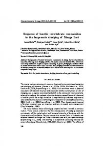
1.1. Schottky system In the standard setting [1 ], a discrete non-equilibrium system G is in interaction with an equilibrium one G∗ , the so-called environment reservoir. The interaction ˙ ∗, between these two systems consists of heat exchange Q˙ ∗ , power exchange W ∗ and material exchanges n˙ , represented by the external mole number rates of the components (see Fig. 1). These kind of discrete systems are called Schottky systems [2 ]. Their exchanges are referred to the equilibrium reservoir G∗ . 1.2. Undecomposed system First of all, we describe the non-equilibrium Schottky system G as an undecomposed one. This means that we are introducing a coarse description ignoring the possible internal structure of the system. It may be composed of different subsystems, but it is described as an undecomposed system, not knowing how the ˙ ∗ , and n˙ ∗ are distributed over the unknown subsystems. exchange quantities Q˙ ∗ , W A prototype for an undecomposed system is the equilibrium environment G∗ . Because of its reservoir properties and the absence of internal adiabatic partitions, G∗ cannot be decomposed into subsystems of different intensive variables. The first law of the open equilibrium reservoir G∗ reads [3 ] ˙ ∗ + h∗ · n˙ ∗ . U˙ ∗ = Q˙ ∗ + W
(1)
Here U ∗ is the internal energy and h∗ are the molar enthalpies of the components of G∗ . The entropy rate of G∗ is that of thermostatics ˙ ∗ µ∗ U˙ ∗ W S˙ ∗ = ∗ − ∗ − ∗ · n˙ ∗ . T T T ∗ Here µ are the chemical potentials of the components of G∗ .
Fig. 1. General structure of a Schottky system (explanations in text). 134
(2)
Inserting the expression for the first law (1) into (2), and introducing the molar entropies s∗ of the chemical components of G∗ , we obtain for the entropy rate Q˙ ∗ S˙ ∗ = ∗ + s∗ · n˙ ∗ , T
s∗ :=
1 (h∗ − µ∗ ) . T∗
(3)
If we describe the system G as an undecomposed one, we have to define its nonequilibrium entropy [4 ]. We do that according to the equilibrium entropy (3)1 of the environment reservoir ´ µ 1 ³˙ Q˙ ˙ S˙ ¤ := Q + h · n˙ − · n˙ =: + s · n. Θ Θ Θ
(4)
Here the coarse non-equilibrium quantities of G have the following meaning: a temperature Θ, the molar enthalpies h, and the chemical potentials µ of the components in G are up to now only symbols which have to be defined later. The molar entropy s of the undecomposed system is defined as in equilibrium according to (3)2 : s :=
1 (h − µ) . Θ
(5)
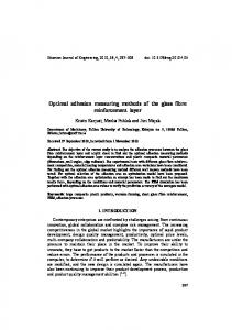
1.3. Endoreversible composite system Up to now, the non-equilibrium system G has been described as an undecomposed system. A more detailed description results from not ignoring that G may be composed . Then G is replaced by the sum of the S of subsystems GjS subsystems G → j Gj . In this case j Gj is called a composite or compound system. In this description, the exchange quantities can be attached to the subsystems. The equivalence of both descriptions with respect to the exchanges is guaranteed by the additivity of the exchanges of the subsystems (see Fig. 2) ˙ ∗ := W
X
˙ j∗ , W
Q˙ ∗ :=
j
X
Q˙ ∗j ,
n˙ ∗ :=
j
X
n˙ ∗j .
(6)
j
By using the additivity conditions (6) we get for the entropy rate (3)1 of the open equilibrium reservoir G∗ X 1 X ˙∗ Qj + s∗ · n˙ ∗j . S˙ ∗ = ∗ T j
(7)
j
135
Fig. 2. Systems G1 and G2 as parts of the composite system G1 ∪ G2 (explanations in text).
S For simplification1 , we consider an endoreversible compound system j Gj which by definition consists of equilibrium subsystems [5 ]. Especially here, these subsystems should be isolated from each other and interact only with their environment G∗ . Because Gj are equilibrium subsystems isolated from each other, their entropy rates are, according to Eq. (3), Q˙ j S˙ j = + sj · n˙ j , Tj
sj :=
¢ 1 ¡ hj − µj . Tj
(8)
Here Tj is the equilibrium temperature of the jth subsystem and sj is its molar entropy. We now need the connection between the heat exchanges Q˙ j with respect to G in (8) and between Q˙ ∗j with respect to G∗ in (7). The connection between these heat exchanges is given by the properties of the partition separating the two systems G and G∗ , which are discussed in the next section.
2. INERT PARTITIONS The heat exchange in open systems is influenced by the material exchange. Therefore the heat exchange has to be redefined for open systems [6 ]. An inert partition which does not absorb or emit heat and material is defined for the jth partition of a composite system by the transfer condition [7 ] Q˙ j + hj · n˙ j := −Q˙ ∗j − h∗ · n˙ ∗j ,
n˙ j := −n˙ ∗j ,
∀j.
(9)
Summing up all partial partitions of the composite system and using the additivity conditions (6), we obtain from relation (9) 1
136
The general case will be treated elsewhere.
X X X (Q˙ j + hj · n˙ j ) = − Q˙ ∗j − h∗ · n˙ ∗j = −Q˙ ∗ − h∗ · n˙ ∗ . j
j
(10)
j
The additivity relations S (6)2,3 of the environment are also valid with respect to the composite system j Gj : X X Q˙ j , n˙ := Q˙ := n˙ j = −n˙ ∗ . (11) j
j
Using the additivity condition (11)1 , we have from (10) X hj · n˙ j = −Q˙ ∗ − h∗ · n˙ ∗ . Q˙ +
(12)
j
By the mean value theorem X hj · n˙ j = h+ · n˙ + + h− · n˙ − ,
n˙ + ≥ 0, n˙ − < 0,
(13)
j
˙ n˙ + + n˙ − = n,
(14)
we obtain from (12), (14), andS(11)2 the transfer condition for an inert partition between the composite system j Gj and the environment G∗ : Q˙ + h · n˙ + (h+ − h) · n˙ + + (h− − h) · n˙ − = −Q˙ ∗ − h∗ · n˙ ∗ .
(15)
If the compound system is described by an undecomposed one, we have to set for G:
˙ h− ≡ ˙ h. h+ ≡
(16)
Consequently, we obtain from (15) the transfer condition for an inert partition between the undecomposed system G and the environment G∗ similarly to (9): Q˙ + h · n˙ = −Q˙ ∗ − h∗ · n˙ ∗ .
(17)
A comparison of (15) with (17) shows that the transfer conditions of composite systems and undecomposed systems differ from each other by the excess term [1 ] H EX := (h+ − h) · n˙ + + (h− − h) · n˙ − ,
(18)
which stems from the different description of the system: as a composite system or as an undecomposed one. In case of an undecomposed system (Eq. (16)), the excess term vanishes. In case of vanishing net material exchange n˙ + + n˙ − = n˙ = ˙ 0,
(19)
the excess term becomes n˙ = ˙ 0:
H EX = (h+ − h− ) · n˙ + .
(20)
For closed systems, it is identical to zero, and the transfer conditions for composite and undecomposed systems are identical in this case. 137
3. TOTAL ENTROPY RATES Taking the transfer condition (9) into account, we obtain from (8) for the sum of entropy rates of the subsystems i X X 1 h S˙ j = −Q˙ ∗j − h∗ · n˙ ∗j − µj · n˙ j . (21) Tj j
j
Together with (7) and (21), the total entropy of the composite system the environment G∗ becomes X S˙ j + S˙ ∗ S˙ tot (T ∗ , µ∗ ) :=
S j
Gj and of
j
¶ ¶ ´ X µµ Xµ 1 1 ³ ˙∗ µ∗ j ∗ ∗ ˙ 0. = − Qj + h · n˙ j + − ∗ · n˙ ∗j ≥ T ∗ Tj Tj T j
(22)
j
The inequality stems from the second law, because of the isolation ofSthe total system. This total entropy appears if we consider the composite system j Gj . Inserting the entropy rate of the undecomposed system (17) into the transfer condition (4), we obtain by using (11)2 and (3) tot S˙ ¤ (T ∗ , µ∗ ) := S˙ ¤ + S˙ ∗ ¶ µ ´ µ µ µ∗ ¶ 1 ³ ˙∗ 1 ∗ ∗ ˙ 0, ˙ − Q + h · n + − · n˙ ∗ ≥ = T∗ Θ Θ T∗
(23)
∗ the total entropy of the undecomposed system S G ∪ G ∗, which is different from the total entropy (22) of the composite system j Gj ∪ G . It follows directly that tot S˙ ¤ (Θ, µ) = 0,
(24)
which is different from S˙ tot (Θ, µ) ≥ 0. tot 6= S˙ tot , we have to introduce the difference of the two Because of S˙ ¤ quantities. This will be done in the next section. 4. EXCESS ENTROPY RATE The entropy rates of the compound system (21) and of the undecomposed system (4) are different. As expected, that means, the entropy rate depends on the description of the system under consideration, as the transfer conditions (15) and (17) do. The difference between entropy rates for the composite system and for the undecomposed system is the excess entropy rate X S˙ j − S˙ ¤ . (25) S˙ EX := j
138
Using (22) and (23), we obtain ¶ ¶ ´ X µµ Xµ 1 1 ³ ˙∗ µ j EX ∗ ∗ ˙ S = − Qj + h · n˙ j + − · n˙ ∗j . Θ Tj Tj Θ j
(26)
j
By comparison with (22), this yields S˙ tot (Θ, µ) = S˙ EX ≥ 0,
(27)
the positive definiteness of the excess entropy rate. According to (26), the minimum of the excess entropy rate appears if the compound system is isolated: Q˙ ∗j = ˙ 0,
n˙ ∗j = ˙ 0, ∀j
→
S˙ EX = 0.
Taking (27) into account, we get from (25) an inequality X S˙ ¤ ≤ S˙ j ,
(28)
(29)
j
which is denoted as sub-additivity of the entropy rates. Sub-additivity is well known for quantum entropies [8 ], but here we proved the sub-additivity of entropy rates for classical systems, which is caused by different descriptions of the same system: the entropy rate of the undecomposed system is smaller than that of the composite system. 5. CONTACT QUANTITIES In this section we will define the symbol introduced in (4) for the coarse nonequilibrium quantities of G. 5.1. Contact temperature If the net material exchange between G and G∗ vanishes, we obtain from (23) a defining inequality [9 ] µ ¶ 1 1 ˙∗ ∗ n˙ = ˙ 0: − Q ≥ 0. (30) T∗ Θ This inequality defines the temperature Θ, unknown up to now: if we contact G – which is in an arbitrary, but fixed non-equilibrium state – by an inert partition which is impervious to material with several G∗ of different temperatures T ∗ , then we find temperatures T1∗ and T2∗ having the following properties: if T1∗ ≤ Θ if T2∗ > Θ
→ →
Q˙ ∗1 ≥ 0, Q˙ ∗2 < 0.
(31) (32) 139
Because there exists exactly one temperature with n˙ ∗ = ˙ 0:
T∗ = Θ
→
Q˙ ∗ = 0,
(33)
we can give [10,11 ]. Definition 1. The contact temperature of G is the thermostatic temperature T ∗ = Θ of the closed controlling reservoir G∗ for which the heat exchange Q˙ ∗ vanishes with the change of its sign. The contact temperature is a non-equilibrium analogue to the thermostatic equilibrium temperature. If G and G∗ are in equilibrium with each other, the contact temperature transfers to the thermostatic temperature. A corresponding defining inequality exists also for the chemical potentials µ, as we will discuss in the next subsection.
5.2. Dynamic chemical potentials The defining inequality for µ follows directly from (23): T∗ = ˙ Θ,
tot S˙ ¤ (Θ, µ∗ ) = (µ − µ∗ ) · n˙ ∗ ≥ 0,
(34)
and we presuppose that this inequality is valid for each component in G: Definition 2. The dynamic chemical potentials µ of G are those chemical potentials µ∗ = µ of the open controlling reservoir G∗ of T ∗ = Θ for which all mole number rates n˙ ∗ vanish with the change of sign. The defining inequalities (30) and (34) introduce the coarse non-equilibrium quantities of the undecomposed system G as special equilibrium quantities of the controlling environment G∗ .
6. COMPOUND DEFICIENCY As we already know from (25), there are excess quantities caused by describing the system with different accuracy [1 ]. Using the defining inequalities, we can derive further inequalities expressing the difference of describing the S undecomposed system G and the composite system j Gj , which is called compound deficiency. For closed systems, we obtain from (22) ˙ 0, ∀j : n˙ ∗j ≡
Q˙ ∗ X Q˙ ∗j − ≥ 0, T∗ Tj j
140
(35)
from (23)
Q˙ ∗ Q˙ ∗ − ≥ 0, T∗ Θ
(36)
Q˙ ∗ X Q˙ ∗j − ≥ 0. Θ Tj
(37)
˙ 0, ∀j : n˙ ∗j ≡ and from (26) ˙ 0, ∀j : n˙ ∗j ≡
j
The last inequality describes clearly what is denoted as compound deficiency: the reduced heat exchange depends on the description of the system as an undecomposed one or as a composite system. From (35) and (37) it follows that X Q˙ ∗j Q˙ ∗ Q˙ ∗ ≥ ≥ . T∗ Θ Tj
˙ 0, ∀j : n˙ ∗j ≡
(38)
j
With the same procedure, from (22) we obtain for systems whose contact temperature is equal to the thermostatic temperature of the environment: T∗ = ˙ Θ:
Q−
µ∗ · n˙ ∗ ≥ 0. Θ
(39)
Here Q is the following abbreviation: ¶ ´ Xµ Xµ 1 1 ³ ˙∗ j Q := − Qj + h∗ · n˙ ∗j + · n˙ ∗j . Θ Tj Tj j
(40)
j
Taking (33) into account, we obtain ´ h∗ X 1 ³ Q = · n˙ ∗ . (µj − h∗ ) · n˙ ∗j − Q˙ ∗j + Tj Θ
(41)
j
From (23) it follows that µ ∗ µ∗ · n˙ − · n˙ ∗ ≥ 0, Θ Θ
T∗ = ˙ Θ: and from (26), T∗ = ˙ Θ:
Q−
µ ∗ · n˙ ≥ 0. Θ
(42)
(43)
Together with (42), this results in T∗ = ˙ Θ:
Q ≥
µ ∗ µ∗ · n˙ ≥ · n˙ ∗ . Θ Θ
If, additionally, also the net material exchange vanishes, we obtain ´ X 1 ³ (µj − h∗ ) · n˙ ∗j − Q˙ ∗j ≥ 0 T∗ = ˙ Θ ∨ n˙ ∗ = ˙ 0: Q = Tj
(44)
(45)
j
141
from which it follows that ∗
T = ˙ Θ ∨ n˙ ∗j = ˙ 0, ∀j :
Q = −
X Q˙ ∗j j
Tj
≥ 0.
(46)
S We now consider a cyclic process in G and in j Gj . Because both systems are endoreversible ones, we obtain from (4) and (21) in case of closed systems: I
n˙ ∗j = ˙ 0, ∀j :
I S˙ ¤ dt = 0 = −
n˙ ∗ = ˙ 0, :
I X
S˙ j dt = 0 = −
Q˙ ∗ dt, Θ I X ˙∗ Qj
j
j
Tj
for G, dt, for
(47)
[
Gj .
(48)
j
Taking (38) into account, these relations result in I
I Q˙ ∗ 0=− dt ≥ − Θ I I X ˙∗ Qj dt ≥ − 0=− Tj j
I ˙ Q˙ ∗ Q dt = dt, for G, T∗ T∗ I ˙ [ Q˙ ∗ Q dt ≥ dt, for Gj . Θ T∗
(49) (50)
j
This is a remarkable result with respect to the compound deficiency: the Clausius inequality of closed systems I ˙ Q dt ≤ 0 (51) T∗ is valid for both descriptions, independently of being undecomposed or composite. In contrast to the general validity of the Clausius inequality, the corresponding inequality, formulated by use of the contact temperature, marks the difference between an undecomposed system and a composite one: I 0 =
Q˙ dt, Θ
I for G,
0 ≥
Q˙ dt, Θ
for
[
Gj .
(52)
j
In any case, the extended Clausius inequalities [12,13 ] I 0 ≥
I ˙ Q˙ Q dt ≥ dt Θ T∗
(53)
are valid for closed systems. The important case for which an undecomposed system is approximately described by only one endoreversible system is discussed in the next section.
142
7. LOCAL EQUILIBRIUM APPROXIMATION A conventional procedure in the description of an irreversible process is the projection of the non-equilibrium state of a system on the state of an accompanying local equilibrium process [14−16 ]. In finite-volume numerical methods such projection is achieved by averaging over the computational cell. This approximation provides the values of local equilibrium parameters in the cell, which are in general different from the values of the contact quantities characterizing the non-equilibrium state of the cell by the exchanges. Here we find a particular situation, where the undecomposed non-equilibrium system is approximated by a local equilibrium (endoreversible) system, the parameters of which are not identical to the corresponding contact quantities due to the averaging procedure. This means that the entropy rate for the undecomposed system is still different from the entropy rate of its endoreversible approximation (cf. (25) for j = 1) S˙ EX := S˙ ? − S˙ ¤ . (54) Here the subscript “?” denotes averaged quantities of the endoreversible approximation. Moreover, inserting the transfer conditions (9) into the expression for the entropy rate excess (26), we obtain in the considered particular case µ ¶ ¶ ´ µµ 1 1 ³˙ µ ? S˙ EX = − − Q? + h · n˙ ? − − · n˙ ? . (55) Θ T? T? Θ Thus, the entropy rate excess is expressed in terms of contact quantities and parameters of the approximating endoreversible system. Using (55), we can rewrite (54) as µ ¶ ¶ ´ µµ 1 1 ³˙ µ ? Q? + h · n˙ ? + S˙ ¤ = S˙ ? + − − · n˙ ? . (56) Θ T? T? Θ The latter means that the local equilibrium approximation of a non-equilibrium state may be true if and only if the local equilibrium values are identical to the values of the corresponding contact quantities. In any other case we need to take the excess quantities into account. 8. DISCUSSION As expected, the description of systems depends on the accuracy of their knowledge. Consequently, the entropy rates of the same system described as an undecomposed one or as a composite system are different and give rise to introduction of the concept of compound deficiency characterized by excess quantities. The intensive non-equilibrium variables of the undecomposed system, 143
such as contact temperature and the dynamic chemical potentials, are defined by inequalities induced by the second law, now proving these well-known inequalities. Another result is the sub-additivity of the entropy rates also for classical systems, which is based on the concept of compound deficiency. Consequently, the subadditivity is caused by the different descriptions of the system and not by the system’s properties themselves. The Clausius inequality for closed systems can be formulated by use of the contact temperature of the non-equilibrium system or by using the thermostatic temperature of the controlling environment reservoir. The value of the Clausius integral formulated with the contact temperature depends, according to (52), on the description, but it is always an upper bound for the usual Clausius integral independently of the chosen description according to (53). The conjecture that these results remain valid also in the case where the compound system is not an endoreversible one, is discussed elsewhere.
ACKNOWLEDGEMENTS Support of the Estonian Science Foundation under grant No. 5765 (A. B.) and discussions with Dipl.-Phys. P. Dedi´e are gratefully acknowledged.
REFERENCES 1. 2. 3. 4. 5. 6. 7. 8. 9. 10. 11. 12. 13.
144
Muschik, W. and Berezovski, A. Thermodynamic interaction between two discrete systems in non-equilibrium. J. Non-Equilib. Thermodyn., 2004, 29, 237–255. Schottky, W. Thermodynamik. Springer, Berlin, 1929. Kestin, J. A Course in Thermodynamics, Vol. I. Hemisphere, Washington, 1979. Muschik, W. Aspects of Non-Equilibrium Thermodynamics. World Scientific, Singapore, 1990. Hoffmann, K.-H., Burzler, J. M. and Schubert, S. Endoreversible thermodynamics. J. NonEquilib. Thermodyn., 1997, 22, 311–355. de Groot, S. R. and Mazur, P. Non-Equilibrium Thermodynamics. North Holland, Amsterdam, 1963. Muschik, W. and G¨umbel, S. Does Clausius’ inequality exist for open discrete systems? J. Non-Equilib. Thermodyn., 1999, 24, 97–106. Breuer, H.-P. and Petruccione, F. The Theory of Open Quantum Systems. Oxford University Press, 2002. Muschik, W. Fundamentals of non-equilibrium thermodynamics. In Non-Equilibrium Thermodynamics with Application to Solids (Muschik, W., ed.). Springer, Wien, 1993, 1–63. Muschik, W. Empirical foundation and axiomatic treatment of non-equilibrium temperature. Arch. Rat. Mech. Anal., 1977, 66, 379–401. Muschik, W. and Brunk, G. A concept of non-equilibrium temperature. Int. J. Eng. Sci., 1977, 15, 377–389. Muschik, W. and Riemann, H. Intensification of Clausius inequality. J. Non-Equilib. Thermodyn., 1979, 4, 17–30. Muschik, W. Extended formulation of the second law for open discrete systems. J. NonEquilib. Thermodyn., 1983, 8, 219–228.
14. Keller, J. U. Ein Beitrag zur Thermodynamik fluider Systeme. Physica, 1971, 53, 602– 620. 15. Muschik, W. Existence of non-negative entropy production. In Proceedings of the 5th International Symposium on Continuum Models of Discrete Systems, Nottingham, 14– 20 July 1985 (Spencer, A. J. M., ed.). Balkema, Rotterdam, 1987, 39–45. 16. Kestin, J. Local-equilibrium formalism applied to mechanics of solids. Int. J. Solids Struct., 1992, 29, 1827–1836.
¨ Mittetasakaalulised kontaktsuurused ja uhenddefitsiit ¨ diskreetsete susteemide piiripindadel Wolfgang Muschik ja Arkadi Berezovski On vaadeldud mittetasakaalulist kontakti inertse vaheseinaga eraldatud kahe ¨ neist − tasakaalus keskkonna ruum − juhib teist diskreetse s¨usteemi vahel. Uks mittetasakaalulist s¨usteemi, mida on kirjeldatud kahel erineval t¨apsuse tasandil: esiteks terviks¨usteemina ja teiseks teineteist mittem˜ojutavatest alams¨usteemidest koosneva p¨oo¨ ratava liits¨usteemina. Terviks¨usteemi muutujate kirjeldused on esitatud p¨oo¨ ratavate alams¨usteemide tasakaalu muutujate kaudu, mis on defineeritud (termod¨unaamika) teisest seadusest tulenevate v˜orratuste kaudu. Liits¨usteemina vaatlemise korral on esitatud muutujad p¨oo¨ ratavate alams¨usteemide tasakaalu muutujate kaudu. Nende kahe kirjelduse erinev t¨apsus viib u¨ henddefitsiidi m˜oisteni. Konkreetsemalt: erinevalt kirjeldatud entroopia m¨aa¨ ra lisandumine on tingitud u¨ henddefitsiidist. L˜opuks: u¨ henddefitsiidi m˜oiste abil on tuletatud seosed suletud s¨usteemide Clausiuse v˜orratuse eri vormide vahel.
145