Full characterization of attractors for two intersected asynchronous Boolean automata cycles
arXiv:1310.5747v1 [cs.FL] 21 Oct 2013
Tarek Melliti1 , Mathilde Noual2 , Damien Regnault1 , Sylvain Sen´e3,4 , and J´er´emy Sobieraj1 ´ ´ IBISC, EA4526, Universit´e d’Evry Val-d’Essonne, 91000 Evry, France ({tarek.melliti, damien.regnault}@ibisc.univ-evry.fr,
[email protected]) 2 I3S, UMR7271 CNRS et Universit´e de Nice Sophia Antipolis, 06900 Sophia Antipolis, France (
[email protected]) 3 Aix-Marseille Universit´e, CNRS, LIF UMR 7279, 13000 Marseille, France (
[email protected]) 4 IXXI, Institut rhˆ one-alpin des syst`emes complexes, 69000 Lyon, France 1
Abstract. Nowadays, the understanding of Boolean automata networks dynamics takes an important place in various domains of computer science such as computability, complexity and discrete dynamical systems. Basing ourselves on these specific mathematical objects, in this paper, we make a step further in this understanding by focusing on their cycles, whose necessity in networks is known as the brick of their complexity. We indeed present new results that provide a characterisation of the transient and asymptotic dynamics, i.e. of the computational abilities, of asynchronous Boolean automata networks composed of two cycles that intersect by sharing one automaton, the so-called double-cycle. Moreover, we introduce here an efficient formalism inspired by algorithms to define long sequences of updates. Also, the analysis of these Boolean automata networks relies on technics developed for cellular automata. These technics allow us to be more precise for describing the asymptotic dynamics than previous works in this area.
Keywords: Boolean automata networks, double-cycles, asymptotic dynamics.
1
Introduction
The part of researches on automata networks currently grows for many reasons. Without being exhaustive, here are two of them, which seems to be the most important to us. First, although this computational model is among the first ones that was developed by precursors like McCulloch and Pitts and their formal neural networks [9], and von Neumann and its cellular automata [11], lots of their intrinsic computational properties are not known nowadays. Second, their
simplicity and the few concepts and parameters needed to define them makes them particularly adapted to capture the essence of and model real interaction systems at a high abstraction level, such as physical, biological and social systems [4,7,19]. The present work precisely takes place at the frontier of theoretical computer science and fundamental bio-informatics, that aims at analysing and explaining formally the dynamics of biological regulations, that have constituted the chore of molecular biology since the results of Jacob and Monod [5,6]. The combination of theoretical computer science and fundamental bio-informatics have given rise to many interesting questions in the two domains. And, in this context, Boolean automata networks play a leading role, through the results that they have allowed to obtain. Indeed, since the seminal works of Kauffman [7,8] and Thomas [20,21] in theoretical biology, computer scientists have not stopped trying to answer their questions/conjectures. Among the latter, those that are central in this work are Thomas’ ones, for which solutions have been proven in the discrete framework at the end of 2000’s, approximately three decades after their formulations, in [15,16,17]. Without entering into details now, these results, together with those of Robert [18], highlighted the fact that the ability of automata networks to admit complex asymptotic behaviours comes from the presence of cycles in their architecture. Since then, scientists have understood that, despite their appearing simplicity, the influence of cycles on networks was not well understood. In particular, no studies have succeeded neither in characterising their dynamical behaviours in terms of enumerative combinatorics (i.e. the number of attractors, their sizes. . . ), until [1] in which the updating mode considered was the parallel one. Then, the same authors attached time to analyse the relations between the dynamical properties of cycles subjected to distinct updating modes, with a special attention paid on the asynchronous and the parallel ones [13]. Once the cycles dynamics finely understood, it seemed natural to dive them in networks architecture in order to make a step towards generality. But obtaining general combinatorial results for any kind of networks remains an open problem that seems intractable actually. So, following a constructive approach and as a first step, studies have been led on specific patterns combining cycles, such as the double-cycles in parallel [1] and the flower-graphs [2] for instance. In addition, other studies have dealt with the convergence time of specific classes of Boolean automata networks, like circular xor networks [14] and networks without negative cycles [10]. In the same lines as these previous works, this paper interests in the dynamical properties of such networks restrained to double-cycles evolving over time according to the asynchronous updating mode. Nevertheless, the methods developed here are original since we show that some recurrent configurations can only be reached by paths of quadratic length according to the size of the networks. First we introduce a formalism to represent efficiently lengthly sequences of updates. This formalism represent them as algorithm. Secondly, we also prove that some recurrent configurations cannot be reached by a path of linear length. Negative results are known to be hard to prove in complexity even basic one. Our results give a more precise characterization of the attractor compared to previous work. They also 2
show that all configurations of the attractor are not equal, some have specific properties. The paper is organized as follows: Section 2 gives the main definitions and notations used in the paper, in particular those related to the double-cycles and to the asynchronous updating mode; Section 3 gives the definition of the tools and methods developed here and finally Section 4 is dedicated to the main contributions of this paper.
2
Definitions and notations
Boolean automata networks. Consider B = {0, 1} and V = {0, . . . , n − 1} a set of n Boolean automata so that ∀i ∈ V, xi ∈ B denotes the state of i. A configuration of a Boolean automata network (a BAN) N of size n is a map from V to B. In other terms, a configuration x ∈ BV instantiates the state of any i of V and is classically denoted as a vector, such that x ∈ Bn , or as a binary word. Formally, a BAN N of size n, whose automata set is V, is a set of n Boolean functions, which means that N = {fi : Bn → B | i ∈ V }. Given i ∈ V, fi is the local transition function of i that predetermines its evolution for any configuration x. Actually, that means that if i is updated in x, its state switches from xi to fi (x). Let us define now the sign of an interaction from j to i (i, j ∈ V) in configuration x ∈ Bn with: signx (j, i) = s(xj ) · (fi (x) − fi (xj )), where s : B → 1l, with 1l = {−1, 1}, is defined as s(b) = b − ¬b, and ∀i ∈ V, xi = (x0 , . . . , xi−1 , ¬xi , xi+1 , . . . , xn−1 ). Interactions that are effective in x belongs to the set A(x) = {(j, i) ∈ V2 | signx (j, i) 6= 0}. From this is derived directly the interaction graph of N that is defined as the digraph G = (V, A), where S A = x∈Bn A(x) is the set of interactions. In this paper, the focus is put on BANs associated with simple interaction graphs, which means that if there exists (j, i) ∈ A, it is unique and such that ∀x ∈ Bn , signx (j, i) 6= 0, and constant. As a consequence, sign(j, i) ∈ 1l. If sign(j, i) = +1 (resp. sign(j, i) = −1), (j, i) is an activating (resp. inhibiting) interaction so that the state of i tends to mimic (resp. negate) that of j. We call the signed interaction graph of N the digraph obtained by labelling each arc (i, j) ∈ A with sign(i, j). In order not to burden the reading, we also denote it by G. Abusing notations, a cycle C of G is said to be positive (resp. negative) if the product of the signs of the interactions that compose equals +1 (resp. −1). Asynchronous transition graphs. In a BAN N , a couple of configurations (x, y) ∈ Bn × Bn , such that y is obtained by updating the state of a unique automaton of x is a asynchronous transition, and is denoted by x y. Thus, if a transition (x, y) is asynchronous then the Hamming distance d(x, y) ≤ 1. y is said to be effective, otherwise, it is said to be ineffecIf x 6= y, x tive. Let T = {x y | x, y ∈ Bn } be the set of asynchronous transitions of 3
N . Digraph G = (Bn , T) is then the asynchronous transition graph (abbreviated simply by transition graph in the sequel) of N , which actually represents the discrete dynamical system related to N subjected to the non-deterministic ”perfectly” asynchronous updating mode. Consider an arbitrary BAN N of size n, its transition graph G = (Bn , T ) and x ∈ Bn any of its possible configurations. A trajectory of x is any path in G that starts in x. A strongly connected component (SCC) of G that admits no outgoing asynchronous transition is a terminal strongly connected component (TSCC). A TSCC of G represents an asymptotic behaviour of N , i.e. one of its attractors. A configuration that belongs to an attractor is a recurrent configuration and, for a given attractor, the number of its configurations is said to be its size. An attractor of size 1 (resp. of size greater than 1) is a stable configuration (resp. a stable oscillation). We close this paragraph by defining the convergence time of a configuration x as the length of the shortest trajectory that leads it to an attractor and the convergence time of a BAN as the biggest convergence time of all configurations in Bn . Boolean automata double-cycles. The literature has put the emphasis on Boolean automata cycles (BACs). The reason comes from the three following theorems that show that cycles are necessary for BANs to admit a complex asymptotic dynamics. Theorem 1. [18] Whatever the updating mode is, a BAN whose interaction graph does not contain any cycle admits a unique attractor, that is a stable configuration. Theorem 2. [15,17,21] Let G be the asynchronous transition graph of a BAN N . If G admits two stable configurations then the interaction graph of N contains a positive cycle. Theorem 3. [15,16,21] Let G be the asynchronous transition graph of a BAN N . If G admits a stable oscillation then the interaction graph of N contains a negative cycle. On the basis of the theorems above, and in the same lines as [1,12] that characterises the dynamical behaviour of Boolean automata double-cycles (BADCs) with the parallel updating mode that leads to get a better understanding of the intrinsic impact of the presence of cycles in BANs, we propose in this paper to study BADCs when updated asynchronously. Informally, a BADC D of size n + m − 1 is composed of two BACs C l (of size n) and C r (of size m) that intersect tangentially on one automaton that will be denoted specifically, for the sake of clarity in proofs, by c (resp. cl0 , cr0 ) when considering D (resp. C l , C r ). Notice that in D, every automaton admits a unary function as its local transition function that is either id or neg, except automaton c that admits a binary function. In this paper, we focus on monotone functions and enforce fc to be a and-function without loss of generality for our concern. Also, remark that there exist three different kinds of BADCs: those made of two positive BACs called 4
+ +
+
+
+
+
− +
+
+
(a)
+
+ (b)
+
− −
+
+
+
+
+
+
(c)
Fig. 1. Interaction graphs of the three kinds of canonical BDACs: (a) a canonical positive BDAC, (b) a canonical mixed BDAC, and (c) a canonical negative BDAC.
positive BADCs, those made of two negative BACs called negative BADCs, and those made of one positive and one negative cycles called mixed BADCs. Furthermore, an interesting point is that the study of BADCs of size n + m − 1 in general can be reduced to that of three canonical BADCs of size n + m − 1 (refer to these two papers cited just above for more details), that are presented in Figure 2. A canonical positive BADC D + is composed only of positive interactions. A canonical negative BADC D − is composed only of positive interactions, except the two that have c as their destination. A canonical mixed BADC D ± is composed only of positive interactions, except one of those that have c as their destination (we suppose that this interaction belong to C l ). To finish, let us explain the specific way chosen to denote an arbitrary configuration x of a BADC. For easing the proofs, we denote it by a vector of two binary words, both in which the first symbol represents xc . For instance, the null configuration in which all automata are at state 0 is denoted by (0n , 0m ). Also, we denote by xl (resp. xr ) the projection of x on cycle C l (resp. C r ), then x = (xl , xr ) and the state of automaton cli in configuration x is xli . To conclude, note that x0 = xl0 = xr0 since these three notations design the state of automaton c in configuration x.
3
Discussion and tools
In this section, we introduce the tools that we will use to study the attractors. In the first part, we introduce the ”expressitivity” of a configuration. This notion counts the number of 01 patterns in a configuration. This notion is inspired by works on asynchronous cellular automata [3] where the number of occurrences of this pattern is generally crucial to understand the behavior of these cellular automata. In the second part, we introduce ”instructions” to represent sequences of updates as classical algorithms. These instructions are useful to express long sequences of updates with only few lines of code. 3.1
Expressivity
First we discuss about the structure of the configurations. We define here a notion of “expressivity” for configurations. 5
Definition 1. For a cycle C of length n , the expressivity of a configuration x of C is the number of 01 patterns along this cycle: |{i : 0 ≤ i ≤ n − 1, xi = 0 and xi+1 mod n = 0}|. For BADC D, the expressivity of a configuration x of D is the sum of the expressivity of xl and xr . This notion is very useful to understand the structure of attractors. The less expressive configurations are (0n , 0m ) and (1n , 1m ) and the most expressive m n m n ones are ((10) 2 , (10) 2 ) and ((01) 2 , (01) 2 ) (if n and m even). On the one hand, we will see that the less expressive configurations are generally recurrent and can be reached in linear time by most configurations. On the other hand, expressive configurations either are not recurrent or can only be reached by very specific sequences of updates but they can quickly reach any other configuration. When there is an attractor of exponential size containing simple and complex configurations, then we conjecture: – the shortest path from a configuration of low expressivity from a high one is linear in n and m; – the shortest path from a configuration of high expressivity to any configuration is linear in n and m. – the shortest path from a configuration of high expressivity from a low one is quadratic in n and m. To summarize, increasing the expressivity is hard but an expressive configuration can reach any other configuration quickly. 3.2
Instructions
In the rest of the article, lots of proofs rely on exhibiting a sequence of updates between two specific configurations. The length of these sequences is problematic. A human reader would not manage to extract the idea of the sequences and the proofs. Thus, we introduce instructions in this section. An instruction is a sequence of updates such that this sequence can be easily defined and its interpretation and effect on the configuration is easy to understand for a human reader. Consider a BDAC D, a cycle C of D, a current configuration x of C and ci and cj automata of C which are not c, we now introduce the different instructions that we will use here: Synchronize: updates automaton c. Update(ci ): updates automaton ci . Clockwise(C , i, j): for k=i to j do Update(ck ). Erase(C ): Clockwise(C , 1, length(C ) − 1). Expand(C ): Clockwise(C , 1, k − 2) where k = min1≤k≤n {k : (xk = x0 ) ∨ (k = n)}. CounterClockwise(C , i, j): for k=j down to i do Update(ck ). Shift(C ): CounterClockwise(C , 1, length − 1). We now discuss the properties and effects of all of these instructions. First note that Synchronize is the only instruction where automaton c is updated and 6
the only instruction where both cycles can interact with each other. In the rest of article, we will always call this instruction when c can switch its state. Synchronize has two ways to be used: the first one is to set the common automaton into a desired state and the second one is to increase the expressivity of a configuration. Instruction Synchronize is the only way to switch a pattern 111 (resp. 000) into a pattern 101 (resp. 010) and thus to increase the expressivity of the configuration. Note that the cycles have to be configure properly to allow automaton c to switch its state. The instruction Update(ci ) updates an automaton which is not c. We will avoid this instruction has much has possible since it does not represent a sequence of updates. We use a specific instruction for automaton c because updating this automaton almost always correspond to key point in algorithms (such as increasing the expressivity of the configuration). The instruction Clockwise(C , i, j) is useful to updates consecutive automata by increasing order. Note that if j < i then no automata are updated and since i is different from 0 then automaton c cannot be updated by this instruction. The aim of Clockwise(C , i, j) is to propagate the state of cj−1 along a cycle: Property 1. Consider a configuration x of cycle C , we denote by x0 the result of applying Clockwise(C , i, j) on x then for all k ∈ {i, . . . , j}, x0k = xi−1 and for all k ∈ / {i, . . . , j}, x0k = xk . We will consider two specific sub case of Clockwise(C , i, j). The first one is Erase(C ). The aim of this instruction is to move information quickly along a cycle: Property 2. Consider a configuration x of cycle C , we denote by x0 the result of applying Erase(C ) on x then for all k ∈ {0, . . . , (length(C ) − 1}, x0k = x0 . Since using this instruction set the expressivity of a cycle to 0, it is really efficient to converge quickly to a fixed point of low expressivity, if this fixed point exists. The second sub case of Clockwise(C , i, j) is Expand(C ). Calling this instruction on cycle C expands the state of c along the cycle until its no more possible to do it without destroying a 01 pattern. The operation Expand does not decrease the expressivity of a configuration but the propagation of the information is stopped along the cycle. This operation is useful to stock the 01 patterns at the end of the cycle and to build expressive configurations. The instruction CounterClockwise(C , i, j) is useful to updates consecutive automata by decreasing order. Note that if j < i then no automata are updated and since i is different from 0 then automaton c cannot be updated by this instruction. The aim of Clockwise(C , i, j) is to make a partial shift of a section of a cycle: Property 3. Consider a configuration x of cycle C , we denote by x0 the result of applying CounterClockwise(C , i, j) on x then for all k ∈ {i, . . . , j}, x0k = xk−1 and for all k ∈ / {i, . . . , j}, x0k = xk . 7
note that the information contained by automaton j is lost and the information contained by i − 1 is now possessed by i − 1 and i. The last instruction Shift(C ) is a special case of CounterClockwise(C , i, j). When Shift(C ) is called on a cycle, all automata of the cycle take the state of its predecessor except automaton c which keeps the same state. Except for the last automaton of the cycle, all information contained along this cycle are kept safe and are only shifted along the cycle. This operation is useful to propagate information along a cycle without losing too much expressivity (at most one pattern 01 is destroyed). Consider a configuration x of a BDAC D and a sequence of updates Sequence(x), from now on, by abuse of notation, we will consider that Sequence(x) designs both a sequence of updates but also the configuration obtained by applying Sequence(x) on configuration x. When we will prove properties on these sequences, x will design the current configuration that evolves according to the different instructions. To conclude this part, we define a more complex sequence of updates called Copy cycle(x, x0 ) (see table 1). This sequence of updates transforms x into x0 if x is expressive enough, this sequence will be useful later. We will use this example to illustrate the expressiveness of our instructions. Table 1. The sequences Copy cycle, Copy and Copy Pair Copy cycle (x, x0 , C i ) 01 - Let n = length(C i ) 02 - If (xin−1 = xin−2 ∧ xin−1 6= x0i n−1 ) Then 03 - Let j = max{xij 6= x0i j }; 04 - Else 05 - Let j = n; 06 - End If 07 - For (k = n − 1) Down To (j + 1) Do 08 - Update(cik−1 ); 09 - Update(cik ); 10 - Done 11 - For (k = j − 1) Down To (1) Do 12 - If (xik 6= x0i k ) Then 13 Update(cik ); 14 - End If 15 - Done
Copy (x, x0 ): 01 - Copy cycle (x, x0 , C l ) 02 - Copy cycle (x, x0 , C r )
Copy Pair (x, x0 ): 01 - If (c 6= c0 ) Then 02 - Shift(C l ); 03 - Shift(C r ); 04 - Synchronize; 05 - End If 06 - Copy(x, x0 ).
Lemma 1. Consider a BADC D and two configurations x and x0 of D such that x0 = x00 then if for all i ∈ {l, r}, x has one of the following properties: 1. for all j ∈ {1, . . . , length(C i ) − 1}, xij 6= xij−1 or 2. for all j ∈ {1, . . . , length(C i )−2}, xij 6= xij−1 and xilength(C i )−1 = x0i length(C i )−1 . 8
3. for all j ∈ {1, . . . , length(C i )−2}, xij 6= xij−1 and there exists k ∈ {1, . . . , length(C i )− 2} such that xik 6= x0i k. then Copy (x, x0 ) = x0 and this sequence consists of at most 2(n + m) updates. Proof. First, note that Synchronize is never called, then at the end of the sequence, we have x0 = x00 by hypothesis. Copy called two times Copy cycle: one time on C l and one time on C r . We have to prove that Copy cycle sets the automata of the cycle given as argument in the correct state. We prove this result for C l . Now we are analyzing Copy cycle. We prove now that at the end of Copy cycle(x, x0 , C l ), we have for all i ∈ {0, . . . , n − 1}, xli = x0li . We proceed in two part, first we prove that at line 10, we have for all i ∈ {j, . . . , n − 1}, xli = x0li (where j is the variable of the algorithm). Secondly, we prove that at line 15, we have i ∈ {1, . . . , n − 1}, xli = x0li and since x0 = x00 all along the algorithm, we can conclude. The two parts of the proof relies on different invariants. We prove the following invariant for the loop For of line 6 for all i ∈ {1, n − j − 1}: Inv1(i): after i iterations of loop For (line 7): automata cln−1 and cln−i−1 have switched their state one time; for all k ∈ {n − i, . . . , n − 2}, cln−1 has switched its state two times. Initialisation: for i = 1, automata cln−1 and cln−i−1 have switched their state one time. Maintenance: suppose that the invariant is true for i ∈ {1, n − j − 1}. For all k ∈ {n − i, . . . , n − 1}, automaton clk are not updated and the properties is true for these automata. Automaton cln−i−2 is updated and its switched its state then the property is true for this automaton. Then, automaton cln−i−1 (which has already switched its states one time) is updated and it will also switched its states (since cln−i−2 has just switched its state for the first time at the previous line). Then the invariant is true for i + 1. Terminaison: Initially xln−1 6= x0ln−1 and by definition of j, xlj 6= x0lj and for all 0 < i < n − j, xln−i = x0ln−i . Since an automaton which switched its state two times come back to its initial state, we have for all k ∈ {j, . . . , n − 1}, xlk = x0lk . Now we focus of the remaining lines of code. Note that, for all 0 < i < j, we have xli 6= xli−1 . We prove the following invariant for the loop For of line 11 for all i ∈ {0, j − 1}: Inv2(i): after i iterations of loop For (line 11): for all k ∈ {j − k, . . . , n − 1}, xlk = x0lk . Initialisation: for i = 0, the proposition is true from the terminaison of Inv1(i). Maintenance: suppose that the invariant is true for i ∈ {0, j − 2}. We have xlj−i−1 6= xlj−i−2 since no automata of i ∈ {1, . . . , j − i} have been updated yet. Then, if xlj−i−1 = x0lj−i−1 then no automaton is updated and the invariant is true for i + 1. If xlj−i−1 6= x0lj−i−1 then the Update of line 13 make xlj−i−1 switched 9
its states into the one of xlj−i−2 6= xlj−i−1 that is to say xlj−i−2 = x0lj−i−1 . In both case, the invariant is true for i + 1. Terminaison: for i = n − 1 at the end of loop For (line 11), xl = x0l . Finally note that an automaton is updated at most two times and thus the length of this sequence is at most 2(n + m).
4 4.1
Results Two positive cycles
It is well known that BADC D + has two fixed points (1n , 1m ) and (0n , 0m ). We use this simple case to introduce our formalism. We give here two sequences of updates (see table 2), one leads to (1n , 1m ) if the configuration has at least one 1 in both cycles, the other one leads to (0n , 0m ) if the configuration is not (1n , 1m ) (in this case we suppose, without lose of generality, that at least one automaton of C l is in state 0). Table 2. Sequences of update : and Fixed0 Fixed1 (x): 01 - If (x0 = 0) Then 02 - find i such xli = 1; 03 - Clockwise(C l , i, n-1); 04 - find j such xrj = 1; 05 - Clockwise(C r , j, m-1); 06 - Synchronize; 07 - End If 08 - Erase(C l ); 09 - Erase(C r ).
Fixed0 (x): 01 - If (x0 = 1) Then 02 - find i such xli = 0; 03 - Clockwise(C l , j, n-1); 04 - Synchronize; 05 - End If 06 - Erase(C l ); 07 - Erase(C r ).
Lemma 2. Let x be a non-stable configuration of BADC D + then Fixed0(x) = (0n , 0m ) and if both cycles possess at least one automaton in state 1 then Fixed1(x) = (1n , 1m ). The convergence time of BADC D + is less than 2(n + m). Proof. Consider a configuration x of BADC D + such it has at least one 1 in both cycles, we study the evolution of x according to the sequence of updates Fixed1(x). At line 1, if x0 = 1 then nothing is done. Otherwise at line 3, we have xln−1 = xli = 1 (see property 1) and at line 5, we have xrm−1 = xrj = 1. Thus after Synchronize of line 6, x0 = 1. Then in every cases at line 7, we have x0 = 1. After instructions Erase(C l ) at line 8 and instruction Erase(C r ) at line 9. We obtain that at the end of the sequence of updates, all automata of x are in the same state as x0 (see property 2) which is 1. The length of this sequence of updates is at most 2(n + m) since each cycle is updated at most two times by different instructions. The study of the sequence of updates Fixed0(x) 10
is almost identical. The only difference is that we need to set xln−1 or xrm−1 to 0 before instruction Synchronize (line 4). 4.2
One positive cycle and one negative cycle
The BADC D ± has one fixed point (0n , 0m ). We give here one sequence of updates which leads to this fixed point from any initial configuration. We call this sequence Simplify (see table 3) since it leads to the least expressive configuration (0n , 0m ). Table 3. The sequences Symplify, Complexify1 and Complexify2 Simplify(x): 1 - If (x0 =1) Then 2 - Erase(C l ); 3 - Synchronize; 4 - End If 5 - Erase(C l ); 6 - Erase(C r );
Complexify2(x): Complexify2(x) 1 - For (i=1) To (n − 1) Do 1 - Synchronize; 2 - Synchronize; 2 - Erase(C r ); l 3 - Expand(C ); 3 - Synchronize; 4 - Erase(C r ); 4 - Expand(C r ); 5 - Done 5 - For (i=1) To (m − 2) Do 6 - Shift(C l ); 7 - Synchronize; 8 - Expand(C r ); 9 - Done
Lemma 3. Let x be a configuration of BADC D ± , Simplify(x) = (0n , 0m ). The convergence time of BADC D ± is less than 2(n + m). Proof. If x0 = 0 at line 1, then x0 = 0 at line 4. If x0 = 1 at line 4 then line 2 switch all automata of C l into state 1 and after the Synchronize of line 3, x0 = 0 since xln−1 = 1. Thus at line 4, we have x0 = 0. Line 5 set all automata of C 1 into state 0 and line 6 set all automata of C 2 into state 0. We conclude that Simplify(x) = (0n , 0m ). The length of this sequence of updates is at most 2(n + m) since each cycle is updated at most two times by different instructions. 4.3
Two negative cycles
Both cycles are even In this part, we will show that for BADC D − if n and m are both even then there is only one attractor of size 2n+m−1 containing all the configurations. In other words, it is possible to reach any configuration from any other configuration. Of course, the convergence time is null. Nevertheless, even if any configuration is accessible from any other one, configurations with high expressivity are hard to reach. To prove the theorem, we will proceed in three parts: 1. we show that any configuration x can reach the less expressive configuration (0n , 0m ) in less than 2(n + m) steps. 11
2. we show that configuration (0n , 0m ) can reach the most expressive configun m ration ((10) 2 , (10) 2 ) in O(n2 + m2 ). m n 3. we show that any configuration can be reached by configuration ((10) 2 , (10) 2 ) in less than 2(n + m) updates. The first point shows that the less expressive configuration is easily accessible from any other configuration. The third point shows that the most expressive configuration can easily reach any configuration. The second point is the hardest part of the proof: we have to reach the most expressive configuration from the less expressive one. This is done using a sequence of updates which is quadratic in the size of n and m. We will later show that this bound is tight and that increasing expressivity of a configuration by δ requires at least δ 2 updates (see lemma 5). We can now describe the sequence of updates for the three different parts. For part 1, the sequence of updates Simplify of the previous case is still efficient to reach the configuration (0n , 0m ). Lemma 4. For any initial configuration x of BADC D − , the sequence of updates Simplify(x) leads to configuration (0n , 0m ) in less than 2(n + m) updates. Proof. The proof of this lemma is exactly the same as lemma 3. The only difference is that (0n , 0m ) is no more a stable configuration. Now, we focus on increasing the expressivity of configuration (0n , 0m ), i.e. we m n give a path from (0n , 0m ) to ((10) 2 , (10) 2 ). We proceed in two steps, the first l step increases the expressivity of C and the second step increases the expressivity of C r without decreasing the expressivity of C l . and finally: Complexify(x)=Complexify2(Complexify1(x)). Lemma 5. For BADC D − , the sequence of updates Complexify1((0n , 0m )) n leads configuration (0n , 0m ) to configuration ((10) 2 , 1m ) in O(n2 +nm) updates. Proof. We prove the following invariant, for i ∈ {1, . . . , n − 1}: Inv(i): after i iterations of loop For, the current configuration is: (1n−i−1 (10)
i+1 2
i
, 1m ) if i is odd and (0n−i−1 (01) 2 0, 0m ) if i is even.
Initialisation: we represent the evolution of the configuration according to the different instructions of the loop: (line 1) Initial configuration: (0n , 0m ); (line 2) Synchronize : (10n−1 , 10m−1 ); (line 3) Expand(C l ) : (1n−1 0, 10m−1 ); (line 4) Erase(C r ) : (1n−1 0, 1m ) and then Inv(1) is true. Maintenance: consider that i is odd, we represent the evolution of the configuration according to the different instructions of the loop: i+1 (line 1) Current configuration: ((1n−i−1 (10) 2 , 1m )); 12
i+1
(line 2) Synchronize : (01n−i−2 (10) 2 , 01m−1 ); i+1 i+1 (line 3) Expand(C l ) : (0n−i−1 (10) 2 , 01m−1 ) = (0n−i−2 (01) 2 0, 01m−1 ); i+1 (line 4) Erase(C r ) : (0n−i−2 (01) 2 0, 0m ) Since i + 1 is even then Inv(i+1) is true. Now consider that i and is even, we represent the evolution of the configuration according to the different instructions of the loop: i (line 1) Current configuration: ((0n−i−1 (01) 2 0, 0m )); i (line 2) Synchronize : ((10n−i−2 (01) 2 0, 10m−1 )); i i (line 3) Expand(C l ) : ((1n−i−1 (01) 2 0, 10m−1 )) = ((1n−i−2 (10) 2 +1 , 10m−1 )); i m n−i−2 (line 4) Erase(C r ) : ((1 (10) 2 +1 , 1 )). Since i + 1 is odd then Inv(i+1) is true. Termination: Inv(i+1) is true for n − 1, thus the configuration at the end of n−1+1 n the loop is ((1n−(n−1)−1 (10) 2 , 1m )) = ((10) 2 , 1m ) and the lemma is true. Moreover since each cycle is updated n times by different instructions, then the length of this sequence of updates is O(n2 + nm). n
Lemma 6. For BADC D − , the sequence of updates Complexify2(((10) 2 , 1m )) n n m leads configuration (10) 2 , 1m ) to configuration ((10) 2 , (10) 2 ) in O(m2 + nm) updates. Proof. We now prove the following invariant, for i ∈ {0, . . . , m − 2}: Inv(i): after i iterations of loop For (line 5), the current configuration is: i+1 n n i ((01) 2 , 0m−i−1 (10) 2 ) if i is odd and ((10) 2 , 1m−i−2 (10) 2 +1 ) if i is even. Initialisation: we represent the evolution of the initial configuration before entering the loop: n Initial configuration: ((10) 2 , 1m ); n (line 1) Synchronize : (00(10) 2 −1 , 01m−1 ); n r −1 (line 2) Erase(C ) : (00(10) 2 , 0m ); n (line 3) Synchronize : ((10) 2 , 10m−1 ); n n r (line 4) Expand(C ) : ((10) 2 , 1m−1 0) = ((10) 2 , 1m−2 (10)). and then Inv(0) is true; Maintenance: consider that i is odd, we represent the evolution of the configuration according to the different instructions of the loop: i+1 n (line 5) Current configuration: ((01) 2 , 0m−1−i (10) 2 ); i+1 n (line 6) Shift(C l ) : (0(01) 2 −1 0, 0m−1−i (10) 2 ); i+1 i+1 n n (line 7) Synchronize : (1(01) 2 −1 0, 10m−2−i (10) 2 ) = ((10) 2 , 10m−2−i (10) 2 ); i+1 i+2 n n (line 8) Expand(C r ) : ((10) 2 , 1m−2−i 0(10) 2 ) = ((10) 2 , 1m−3−i (10) 2 ); since i + 1 is even then Inv(i+1) is true. Now consider that i and is even, we represent the evolution of the configuration according to the different instructions of the loop: n i (line 5) Current configuration: ((10) 2 , 1m−i−2 (10) 2 +1 ); n i (line 6) Shift(C l ) : (1(10) 2 −1 1, 1m−i−2 (10) 2 +1 ); n i n i (line 7) Synchronize : (0(10) 2 −1 1, 01m−i−3 (10) 2 +1 ) = ((01) 2 , 01m−i−3 (10) 2 +1 ); n i (line 8) Expand(C r ) : ((01) 2 , 0m−i−2 (10) 2 +1 ); 13
since i + 1 is odd then Inv(i+1) is true. Termination: Inv(i+1) is true for n − 1, thus the configuration at the end m−2 n n m of the loop is ((10) 2 , 1m−(m−2)−2 (10) 2 +1 ) = ((10) 2 , (10) 2 ) and the lemma is true. Moreover since each cycle is updated m times by different instructions, then the length of this sequence of updates is O(m2 + nm). By combining the two previous lemma, we obtain the following one. Lemma 7. For BADC D − , the sequence of updates Complexify((0n , 0m )) m n leads configuration (0n , 0m ) to configuration ((10) 2 , (10) 2 ) in O(l2 ) updates. Now, we give the last sequence of updates which for any configuration x0 m n transforms ((10) 2 , (10) 2 ) into x0 . To achieve this goal, we only have to correctly initialize the configuration before using Copy, this is can be done using Copy Pair (see table 1) . n
m
Lemma 8. For BADC D − , the sequence of updates Copy Pair(((10) 2 , (10) 2 ), x0 ) m n leads configuration ((10) 2 , (10) 2 ) to configuration x0 in at most 2(n + m) updates. Proof. If x00 = 1 then the evolution of the configuration according to the different instructions from line 1 to 5 is : m n Initial configuration: ((10) 2 , (10) 2 ); m n (line 2) Shift(C l ) : (1(10) 2 −1 1, (10) 2 ); n m (line 3) Shift(C r ) : (1(10) 2 −1 1, 1(10) 2 −1 1); n m m n (line 4) Synchronize : (0(10) 2 −1 1, 0(10) 2 −1 1) = ((01) 2 , (01) 2 ). Then at line 5, in every case we have x0 = x00 and for all i ∈ {1, . . . , n}, xli 6= xli−1 and for all j ∈ {1, . . . , m}, xri 6= xri−1 . We can directly conclude using lemma 1. Finally for any configuration x and x0 , we have the following properties: Copy Pair((Complexify(Simplify(x))), x0 ) = x0 and thus the following theorem is deduced from the three precedent lemma. Theorem 4. For BADC D − , if n and m are even, then there is one attractor of size 2n+m−1 containing all the configurations. Moreover, any configuration can reach any other configuration in O(n2 + m2 ) updates. Configurations (0n , 0m ) and (1n , 1m ) can be reached from any configuration in at most 2(n + m) updates n m n m and configurations ((10) 2 , (10) 2 ) and ((01) 2 , (01) 2 ) can reach any other configuration in less than 2(n + m) updates. Now we will prove that the bound of O(n2 + m2 ) is tight. Theorem 5. Consider configuration x any sequence of updates which increases the expressivity of a cycle of x by δ is of size Ω(δ 2 ). 14
Proof. Consider a configuration x, without loss of generality we suppose that we increase the complexity of C l by δ. The only way to increase the complexity of C l is by using Synchronize but note that doing two Synchronize will leads c0 into its initial state. Moreover, consider the following sequence for i ∈ {1, . . . , n}. Synchronize Clockwise(C l , 1, i) Synchronize Clockwise(C l , 1, i) Then the first call to Clockwise is useless since the second call to Clockwise will erase all the information contained by automata cl1 , . . . , cli . Thus the δ calls to instruction Synchronize which are needed to increase the expressivity of the configuration are separated by updates which propagate along the cycle the patterns created by the previous calls to instruction Synchronize. Since there is at least δ calls to instruction Synchronize, the pattern created the ith times this instruction is called has to be propagated at least to automaton clδ−i−1 . Thus the ith times Synchronize is called, at least δ − 1 updates are needed to save the pattern created by the instruction. At the end Ω(δ 2 ) updates are needed to increase the expressivity of the configuration by δ. And the following corollary is obtained with x = (0n , 0m ), δ = r δ=m 2 for C . n
n 2
for C l and
m
Corollary 1. Reaching ((10) 2 , (10) 2 ) from (0n , 0m ) requires Θ(n2 +m2 ) steps. At least one odd cycle Let we now consider BADCs D − with at least one odd cycle. As the even case, D − has only one attractor. But unlike the even case we have a non empty set of configurations that do not belong to the attractor. Such configurations are called irreversible. The following lemma characterize them. Lemma 9. Let we consider a BADCs D − with at least one odd cycle. 1. If C i is an odd cycle of size k > 1 then any update of a configuration x s.t k xi = (10) 2 1 is irreversible. − 2. If D is composed of two odd cycles of sizes n > 1 and m > 1, then the n m update of the configuration ((01) 2 0, (01) 2 0) is irreversible. Proof. To prove this lemma we will proceed in two steps. First we prove the n irreversibility of the configurations of the form ((10) 2 1, −) when n is odd, then n m we prove the irreversibility of ((01) 2 0, (01) 2 0) when both cycles are odd. n
Irreversibility of ((10) 2 1, −) : In order to simplify this proof, let we consider a BAN composed by a negative odd cycle, let say C of size n and an automata c∗ s.t fc0 = cn−1 ∧ c∗ , fc∗ = ¬c∗ and fci = ci−1 for i = 1 . . . n − 1. We note the configurations of this BAN by a couple as for BADCs in the following form (c∗ , c0 . . . cn−1 ) Let we consider the n configuration x = (−, (10) 2 1) and let x0 = Update(ci ) for some i = 0 . . . n − 1. 15
We show here that there is no sequence of updates that allows a going back to x from x0 . Let we suppose the existence of a sequence, let say σ, made up of Update() and Synchronize actions, that allows to reach x from x0 . When i = 1..n − 1 we have x0i = x0i−1 which means that to reach x the sequence σ contains at least one Update(ci−1 ). By iterating the argument we can deduce that at least one Synchronize appears in σ i.e the path to x passes through a configuration where c0 = 0. While x0n−1 = 1, in order to reach x, σ must contains also at least an Update(cn−1 ) i.e σ passes through a configuration where the cn−1 = 0. For the case where i = 0 or i = n − 1 it is obvious that σ will also passes through a configuration where cn−1 = 0. So, any sequence that leads to x from x0 passes through a configuration with cn−1 = 0. We can then have the two following statements about σ: (a) Any σ that reaches x from x0 must contains at least one Update(cn−1 ) (b) Any time σ passes through a configuration where c0 = 0 and cn−1 = 1, then after that configuration σ contains at least two occurrences of Update(cn−1 ). Let we now focus on the postfix of σ that begins within the last occurrence of Update(cn−1 ). According to (a) such postfix exists. Also according to (b) the postfix does not contain any Synchronize. Indeed, if the postfix contains a Synchronize, this means that the postfix passes through a configuration with c0 = 0, since cn−1 = 1, according to (b) the postfix must then contains at least two occurrences of Update(cn−1 ) which contradict the fact that we consider the postfix with the last Update(cn−1 ). Let x00 be the configuration reached after the last Update(cn−1 ) of σ, we have then x000 = 1 and x00n−1 = 1. In the case where, n > 1 (c0 and cn−1 are two different automata), we must also have x00n−2 = 1 and x00n−3 = 0 and so on. This means x00n−i = 0 for i odd. While n is odd then x000 = 0 which is a contradiction. x00 does not exist and so σ. n What we just proved is that the configuration (10) 2 1 can not be reached ∗ even by having the total freedom to fix the value of c . In the case of the two cycles with at least one odd, let say C l , crm−1 plays the role of c∗ . The updates of crm−1 are more restricted since they depend on the configuration of C r and n indirectly depend on C l . So, If we can not reach (10) 2 1 by the use of c∗ then r we can not reach it using C . n
m
Irreversibility of of ((01) 2 0, (01) 2 0) : Let we now consider a BADC D − where n and m are both odd and greater n n than 1. The proof of irreversibility of ((01) 2 0, (01) 2 0) can be done by contradiction as for the previous one. Let we consider the configuration x0 resulted from the update of one automata n n from the configuration x = ((01) 2 0, (01) 2 0). By using the same argument, we can state that any path that can reaches x from x0 must passes through a configuration with c0 = 0 and cln−1 = 1 or crm−1 = 1. Consider now the last 16
occurrence of Update(cln−1 ) or Update(crm−1 ). After such occurrence we have (i) no Synchronize will occurs (ii) the reached configuration y 6= x with y0 = 0, l r l l yn−1 = 0, x00r m−1 = 0 and (iii) either ym−2 = 0 or yn−2 = 0. Let say yn−2 = 0 this l means yn−3 = 1 and by iterating the argument we conclude that y0 = 1 which contradict the fact that their is no Synchronize after that last occurrence of Update(cln−1 ) or Update(crm−1 ). Let I be the set of irreversible configurations of a BADCs D − according to lemma 9. We notice that at least one of the most expressive configurations is no longer reachable from (0n , 0m ) since it belongs to I. If we ignore the configuration in I, the most remaining expressive configurations are: m n m n (a) ((10) 2 0, (10) 2 ) and ((01) 2 0, (01) 2 ) for the case of only one odd cycle. m n m n (b) ((10) 2 0, (10) 2 0) and ((01) 2 1, (01) 2 0) for the case of two odd cycles. The sequences Shift(C l ); Shift(C r ); Synchronize; and Shift(C l );Shift(C r ); Update(cln−1 );Update(crm−1 );Synchronize; allow to switch between the expressive configurations of, respectively, the case (a) and (b). It is easy to check m n that the application of Complexify on (0n , 0m ) leads to ((01) 2 0, (01) 2 ) in the n m case (a) and ((01) 2 1, (01) 2 0) in the case (b). This means that in every case we can construct a sequence to move from any configuration to another if and only if they are not in I. The length of these sequences is quadratic as the previous case. We give now a generalization of theorem 4 for any type of negative BADC. Theorem 6. Let α : N → {0, 1} with α(n) = 0 if n = 0 or odd and 1 otherwise. For BADC D − , there is one attractor of size 2n+m−1 − |I| where |I| = α(n − 1) ∗ 2m−1 − α(m − 1) ∗ 2n−1 . Moreover, any two configurations which are not in I can reach each others in Θ(n2 + m2 ) updates. Proof. We first proof the existence of only one attractor made up of all configurations but I, then we sketch the size of I. Let x and y be two configurations with x 6∈ I and y 6∈ I. It is easy to see that Simplify(x) = (0n , 0m ). We consider two cases (a) only one odd cycle let say C l and (b) two odd cycles : (a) In this case the most complex configurations other then I are either x1 = n m n m ((10) 2 0, (10) 2 ) or x0 = ((01) 2 0, (01) 2 ). One can check that the sequence Shift(C l ),Shift(C r ), Synchronize allows to switch from x1 to x0 and vice versa. m n (b) The most complex configuration other than I are x1 = ((10) 2 0, (10) 2 0) n m and x0 = ((01) 2 1, (01) 2 0). Again the sequence Shift(C l ), Shift(C r ), Update(cln−1 ), Update(crm−1 ), Synchronize allows to switch from x1 et x0 and vice versa. One can check easily that for the both cases we have Complexify((0n , 0m )) = x0. We create a new version of Complexify that takes as parameter a configuration and either 1 or 0 with Complexify(z, 0) = Complexify(z) and Complexify(z, 0) = Complexify(z) followed by the switch sequence depending on the case (a) or (b). We have now y and Complexify((0n , 0m ), y0 ) valid 17
the hypotheses of Copy cycle. So we have y = Copy cycle (Complexify (Simplify(x), y0 ), y). The complexity of the sequence to move from x to y is the same as the even case which is determined by the complexity of Complexify which is Θ(n2 + m2 ). We have just proved that all the configurations but I form an attractor. So if we determine the size of I we obtain the size of the attractor. As states in lemma 9, the size of I depends on the number of odd cycles. For the case with only one odd cycle, let say C l is odd, the set I is composed by configuration n of the form ((10) 2 1, −) i.e |I| = 2m−1 . For the second case, two odd cycles, I n m is composed by configuration of the form ((10) 2 1, −) or (−, (10) 2 1) and the n m configuration ((01) 2 0, (01) 2 0) i.e |I| = 2m−1 +2n−1 +1. Since the configuration m n ((10) 2 1, (10) 2 1) was counted twice we subtract one which means that |I| = 2m−1 + 2n−1 . In the case where the size of the odd cycle is 1 the irreversible configuration do not exists this is guaranteed by the fact that α(0) = 0.
References 1. Demongeot, J., Noual, M., Sen´e, S.: Combinatorics of Boolean automata circuits dynamics. Discrete Applied Mathematics 160, 398–415 (2012) ´ Relations between gene regulatory networks and cell dynam2. Didier, G., Remy, E.: ics in Boolean models. Discrete Applied Mathematics 160, 2147–2157 (2012) 3. Fat`es, N., Regnault, D., Schabanel, N., Thierry, E.: Asynchronous behaviour of double-quiescent elementary cellular automata. In: Proc. of LATIN’2006. LNCS, vol. 3887. Springer (2006) 4. Ising, E.: Beitrag zur theorie des ferromagnetismus. Zeitschrift f¨ ur Physik 31, 253– 258 (1925) 5. Jacob, F., Monod, J.: Genetic regulatory mechanisms in the synthesis of proteins. Journal of Molecular Biology 3, 318–356 (1961) 6. Jacob, F., Perrin, D., Sanchez, C., Monod, J.: L’op´eron: groupe de g`enes a ` expression coordonn´ee par un op´erateur. Comptes rendus hebdomadaires de l’Acad´emie des sciences 250, 1727–1729 (1960) 7. Kauffman, S.A.: Metabolic stability and epigenesis in randomly constructed genetic nets. Journal of Theoretical Biology 22, 437–467 (1969) 8. Kauffman, S.A.: Current topics in developmental biology, vol. 6, chap. Gene regulation networks: A theory for their global structures and behaviors, pp. 145–181. Elsevier (1971) 9. McCulloch, W.S., Pitts, W.H.: A logical calculus of the ideas immanent in nervous activity. Bulletin of Mathematical Biophysics 5, 115–133 (1943) 10. Melliti, T., Regnault, D., Richard, A., Sen´e, S.: On the convergence of Boolean automata networks without negative cycles. In: Proceedings of AUTOMATA. Lecture Notes in Computer Science, vol. 8155, pp. 124–138. Springer (2013) 11. von Neumann, J.: Theory of self-reproducing automata. University of Illinois Press (1966) 12. Noual, M.: Dynamics of circuits and intersecting circuits. In: Proceedings of LATA. Lecture Notes in Computer Science, vol. 7183, pp. 433–444. Springer (2012) ´ 13. Noual, M.: Updating automata networks. Ph.D. thesis, Ecole normale sup´erieure de Lyon (2012)
18
14. Noual, M., Regnault, D., Sen´e, S.: About non-monotony in Boolean automata networks. Theoretical Computer Science ´ Ruet, P., Thieffry, D.: Graphic requirement for multistability and attrac15. Remy, E., tive cycles in a Boolean dynamical framework. Advances in Applied Mathematics 41, 335–350 (2008) 16. Richard, A.: Negative circuits and sustained oscillations in asynchronous automata networks. Advances in Applied Mathematics 44, 378–392 (2010) 17. Richard, A., Comet, J.P.: Necessary conditions for multistationarity in discrete dynamical systems. Discrete Applied Mathematics 155, 2403–2413 (2007) 18. Robert, F.: Discrete iterations: a metric study. Springer Verlag (1986) 19. Schelling, T.C.: Dynamic models of segregation. Journal of Mathematical Sociology 1, 143–186 (1971) 20. Thomas, R.: Boolean formalization of genetic control circuits. Journal of Theoretical Biology 42, 563–585 (1973) 21. Thomas, R.: On the relation between the logical structure of systems and their ability to generate multiple steady states or sustained oscillations. In: Numerical methods in the study of critical phenomena, Springer Series in Synergetics, vol. 9, pp. 180–193. Springer-Verlag (1981)
19