Can. J. Remote Sensing, Vol. 33, No. 2, pp. 81–87, 2007
Full fuzzy land cover mapping using remote sensing data based on fuzzy c-means and density estimation Anil Kumar, S.K. Ghosh, and V.K. Dadhwal Abstract. The three stages in supervised digital classification of remote sensing data are training, classification, and testing. The commonly adopted approaches assume that boundaries between classes are crisp and hard classification is applied. In the real world, however, as spatial resolution decreases significantly, the proportion of mixed pixels increases. This leads to vagueness or fuzziness in the data, and in such situations researchers have applied the fuzzy approach at the classification stage. Some researchers have tried fuzzy approaches at the training, classification, and testing stages (full fuzzy concept) using statistical and artificial neural network methods. In this paper a full fuzzy concept has been presented, at a subpixel level, using density estimation using support vector machine (D-SVM) and fuzzy c-means (FCM) approaches. These approaches (SVM and FCM) were evaluated with respect to a fuzzy weighted matrix. In this test study using a four-channel dataset, a comparison of methods has found that a D-SVM function using a Euclidean norm yields the best accuracy. Résumé. Les trois étapes de la classification numérique dirigée des données de télédétection sont l’entraînement, la classification et la validation. Les approches adoptées généralement supposent que les frontières entre les classes sont nettes et on applique ainsi des classifications dures. Toutefois, dans la réalité, lorsque la résolution spatiale diminue significativement, la proportion de pixels mixtes augmente. Ceci entraîne une imprécision ou un flou dans les données et, dans de tels cas, les chercheurs ont appliqué une approche floue au stade de la classification. Certains chercheurs ont essayé des approches floues aux stades de l’entraînement, de la classification et de la validation (concept flou complet) utilisant des méthodes statistiques et des réseaux de neurones artificiels. Dans cet article, un concept flou complet est présenté, au niveau du sous-pixel, basé sur l’utilisation des approches D-SVM de même que FCM. Ces approches (SVM et FCM) ont été évaluées par rapport à la matrice floue pondérée. Dans cette étude test, basée sur l’utilisation d’un ensemble de données de quatre bandes, une comparaison des méthodes a montré qu’une fonction D-SVM utilisant une norme euclidienne donne la meilleure précision. [Traduit par la Rédaction]
Introduction
Kumar et al.
87
Remotely sensed data of the earth may be analyzed to extract useful thematic information. Multispectral classification is one of the most often used methods for information extraction. This procedure assumes that imagery of a specific geographic area is collected in multiple regions of the electromagnetic spectrum. In supervised classification, the identity and location of some of the land cover types are known a priori. The analyst attempts to locate specific sites in the remotely sensed data that represent homogeneous examples of known land cover types. These areas are commonly referred to as training sites and are based on the multivariate statistical parameters, i.e., means, standard deviations, covariance matrices, correlation matrices, etc., of each training site (Jensen, 1996). The classification algorithm is trained to perform land cover classification of the rest of the image. This classification method allocates only the class that dominates that pixel, however, and ignores other classes within that pixel. This leads to a loss of information when there are mixed pixels. To account for information within mixed pixels, hard classifiers are inadequate, and an analyst must resort to a different category of classifiers known as soft classifiers that account for the mixed proportions within a pixel. These © 2007 CASI
classifiers are based on fuzzy set theory, neural networks, or a linear mixture model. Fuzzy set classification takes into account the heterogeneous and imprecise nature of the real world and may be used in conjunction with supervised classification algorithms. The instantaneous field of view (IFOV) of a sensor system normally records the reflected or emitted radiant flux from heterogeneous mixtures of biophysical materials such as soil, water, rock, and vegetation. Also, land cover classes usually grade into one another without sharp, hard boundaries. Thus, in the real world, information on the ground is imprecise and heterogeneous (Wang, 1990a; 1990b; Lam, 1993). Unfortunately, we usually use very precise classical set theory to classify remotely sensed data into discrete, homogeneous information classes, ignoring the imprecision found in the real world. Instead of being Received 10 November 2005. Accepted 29 January 2007. A. Kumar1 and V.K. Dadhwal. Indian Institute of Remote Sensing, Department of Space, Government of India, 4 Kalidas Road, Dehradun 248001, Uttarakhand, India. S.K. Ghosh. Department of Civil Engineering, Indian Institute of Technology, Roorkee, Roorkee 247 667, Uttarakhand, India. 1
Corresponding author (e-mail:
[email protected]). 81
Vol. 33, No. 2, April/avril 2007
assigned to a single class out of m possible classes, each pixel in a fuzzy classification has m membership grade values, each associated with how probable (or correlated) it is with each of the classes of interest. This information may be used by the analyst to extract more precise land cover information, especially concerning the makeup of mixed pixels (Fisher and Pathirana, 1990; Foody and Trodd, 1993). Many researchers have applied fuzzy methods at the training, classification, and testing stages of classification using statistical and artificial neural network approaches (Zhang and Foody, 2001). The aim of this paper is to carry out a comparative study of a full-fuzzy land cover mapping technique using the fuzzy c-means (FCM) and density estimation using support vector machine (D-SVM) approaches with respect to overall soft classification accuracy. The essence of this paper lies in the use of statistical learning, the D-SVM approach algorithm, for subpixel classification. The D-SVM approach algorithm uses mean field (MF) theory for developing an easy and efficient learning procedure for the SVM. This algorithm approximates the distribution of the SVM parameters as a Gaussian process and uses the MF theory to easily estimate learning parameters. The algorithm selects the weights of the mixture of kernels used in the SVM estimate more accurately and faster than traditional quadratic programming-based algorithms (Refaat and Farag, 2004). The supervised subpixel classification output from the D-SVM approach can be effectively evaluated using a fuzzy error matrix (FERM) (Binaghi et al., 1999) and compared with the FCM approach while using different norms of a fuzzy weight matrix. None of the currently available commercial digital image processing software packages include full fuzzy classification algorithms for remote sensing data. Thus an in-house software package, known as the subpixel multispectral image classifier (SMIC), was used (Kumar et al., 2006). This software package has the capability to incorporate training data in pure and mixed modes. Using pure or mixed data, the SMIC package has the capability to identify feature vectors into hard or subpixel classification output. For assessment of classification accuracy, the software package uses the traditional error matrix and the kappa coefficient (Khat) and FERM (Binaghi et al., 1999) for subpixel classified output.
training stage, the fuzzy parameters were generated as follows. Fuzzy set theory has been used to compute fuzzy mean and fuzzy covariance matrices. For example, the fuzzy mean v*c can be expressed as follows (Wang, 1990a): n
v*c =
Fuzzy c-means
i =1 n
(1)
∑ fc(xi) i =1
where n is the total number of sample pixel measurement vectors, fc is the membership function of class c, and xi is a sample pixel measurement vector (1 ≤ i ≤ n). The fuzzy covariance matrix Vc* is computed as follows: n
Vc* =
∑ fc(xi)(xi − v*c)(xi − v*c)T i =1
n
(2)
∑ fc(xi) i =1
When calculating a fuzzy mean for class c, each sample pixel measurement vector x is multiplied by its membership grade in class c, fc(x), before the summation is carried out. Similarly, when calculating a fuzzy covariance matrix for class c, (xi – v*c )(xi – v*c )T is multiplied by fc(x) before being added. To perform a fuzzy feature partition at the classification stage, a membership function must be defined for each class. Equation (3) shows the formula for generating membership values (µij), and A* is a fuzzy weight matrix and is known as the weight matrix A: 1
µ ij =
d2 ∑ d ij2 k =1 ik c
1 (m−1)
(3)
where c
dik2 = ∑ dij2
(4)
j =1
Full fuzzy supervised approaches Different algorithms for multispectral image classification can be used for full fuzzy land cover mapping. Full fuzzy supervised classification of suburban land cover from remotely sensed imagery can be undertaken using statistical and artificial neural networks (Zhang and Foody, 2001). Two methods have been used in this paper for full fuzzy land cover mapping and are discussed in the following sections.
∑ fc(xi) xi
and 2 dij2 =| | x i − v*j | | A = (x i − v*j ) T A*(x i − v*j )
(5)
Three A norms (Euclidean, Diagonal, and Mahalonobis), each induced by a specific weight matrix, are used in this paper to see the effect of these norms on classification results. The matrix A controls the shape of the optimal clusters. The formulations of each norm are given as follows (Bezdek, 1981):
The fuzzy c-means method involves the generation of fuzzy parameters for training, classification, and testing. At the 82
© 2007 CASI
Canadian Journal of Remote Sensing / Journal canadien de télédétection
A* = I
(Euclidean norm)
A* = D −j 1
(Diagonal norm)
A* = C −j 1
(Mahalonobis norm)
K*(x, xi) = exp[–0.5(x – xi)(A*)–1(x – xi)T]
where I is the identity matrix, and Dj is the diagonal matrix having diagonal elements as the eigenvalues of the variance covariance matrix Cj, given by N
C j = ∑ (x i − v*j )(x i − v*j ) T
(9)
(6)
(7)
where fuzzy weighted matrices A* have three norms as described in Equation (6). Based on Equation (8), the definition of the membership function for class c can be defined as follows: µ c (x) =
p*c (x) c
∑
(10)
Pi*(x)
i =1
i =1
where v*j is the fuzzy mean for the jth class. Fraction images can be generated for each lass using Equation (3).
where c is the number of classes, and 1 ≤ i ≤ c. Fraction images can be generated for each class using Equation (10), and the proportion of mixed class information can be obtained from these fraction images.
Density estimation A novel algorithm for the D-SVM approach was used in this study, and the MF theory was used for developing an easy and efficient learning procedure for the SVM (Refaat and Farag, 2004). Consequently, the estimate of the fuzzy density function, P*(x), can be expressed in the form n
P*(x) = ∑ w i K*(x, x i)
(8)
i =1
where wi is the learning weight, and K*(x, xi) is called a kernel function in SVM terminology. In this study, a fuzzy Gaussian kernel K*(x, xi) has been used as follows:
Study area and data used The present study area is in the Dehradun district of Uttarakhand State, India, and is bounded by latitudes 30°23′31.83′′ N to 30°25′43.33′′ N and longitudes 77°46′00.64′′ E to 77°51′07.03′′ E. The study area is part of the rural area of the district and is shown in Figure 1. The climate is generally temperate but varies greatly from tropical to severe cold depending on elevation. Temperature variations due to differences in elevation are considerable. Summers are pleasant in the hilly regions, but the heat is often intense during the summer in the plains areas of the district. The area receives an average annual rainfall of 2073.3 mm, which occurs primarily during the period June to September.
Figure 1. Location of the study area. © 2007 CASI
83
Vol. 33, No. 2, April/avril 2007 Table 1. Details of the training dataset. Type of data used
No. of pixels used
Pure pixels for different classes Agriculture Fallow land Forest Sand Water Mixed pixels for training
58 42 43 41 41 54
Land cover is mixed and includes forest, water, agriculture, fallow land, and sandy areas. A LISS-III four-channel image acquired by the Resourcesat-1 (IRS-P6) satellite on 4 November 2003 was used in the analysis. The image has 250 rows and 296 columns, with a spatial resolution of 23.5 m. The image contains approximately 30% forest, 30% agriculture land, 15% fallow land, 15% sand, and 10% water (Figure 1).
Training and reference dataset collection Sample training data for all five classes were collected from the imagery with reference to topographic maps and using a global positioning system (GPS) to assist in the field. Fuzzy statistical parameters were calculated using these reference datasets. The number of samples for training was greater than
10n per class (Jensen, 1996), where n is the dimensionality of the data (i.e., the number of pixels used) (Table 1). Reference data in the form of fraction images derived from the LISS-IV sensor of the Resourcesat-1 (IRS-P6) satellite were used to assess accuracy. LISS-IV sensor data were acquired for the same date as the LISS-III data. A total of 120 testing pixels per class were randomly selected from each class from corresponding outputs and their reference images, respectively, which is significantly larger than the sample size of 75–100 pixels per class as recommended by Congalton (1991) for the purpose of accuracy assessment.
Data analysis Using the training data in Table 1, fuzzy statistical parameters (e.g., fuzzy means and fuzzy variance–covariance) have been generated using Equations (1) and (2). In the FCM algorithm, fuzzy statistical parameters have been used to generate class membership values using Equation (3), using different norms of the weighted matrix A as defined by Equation (6). Using membership values, output has been generated in the form of fraction images (Figure 2). The FCM using the Euclidean norm gives a higher accuracy than those using the diagonal and Mahalonobis norms (Table 2). The FCM classifier using either the diagonal norm or the Mahalonobis norm was observed to give more misclassification for the forest and water classes compared with the Euclidean norm.
Figure 2. Fraction images generated from the FCM subpixel classification algorithm using different norms: (a) Euclidean norm; (b) Diagonal norm; (c) Mahalonobis norm. 84
© 2007 CASI
Canadian Journal of Remote Sensing / Journal canadien de télédétection Table 2. User’s, producer’s, and overall accuracies (%) for the FCM subpixel classifier. Accuracy–class User’s accuracy Agriculture Fallow land Forest Sand Water Producer’s accuracy Agriculture Fallow land Forest Sand Water Overall accuracy
Euclidean norm
Diagonal norm
Mahalonobis norm
86.04 94.17 95.97 93.18 94.01
94.18 65.05 99.25 98.49 88.44
92.22 65.95 98.61 95.54 76.91
98.53 82.38 93.09 94.77 95.51 92.33
93.19 98.72 83.44 81.65 96.69 89.42
84.72 94.72 80.55 85.87 97.97 86.65
The D-SVM has been implemented such that fuzzy weighted matrices have been used to define the fuzzy Gaussian kernel. The membership values have been calculated using Equation (10), and the corresponding fraction images have been generated (Figure 3). It is observed that the Euclidean norm again gives better results than the other two norms (Table 3). It is also observed that the number of misclassifications decreases in the case of forest and water classes when the diagonal and Mahalonobis norms are used for the D-SVM approach.
Table 3. User’s, producer’s, and overall accuracies (%) for the SVM subpixel classifier. Accuracy–class User’s accuracy Agriculture Fallow land Forest Sand Water Producer’s accuracy Agriculture Fallow land Forest Sand Water Overall accuracy
Euclidean norm
Diagonal norm
Mahalonobis norm
88.40 99.82 99.82 96.77 99.99
100.00 100.00 100.00 66.26 84.95
76.16 79.32 97.31 89.25 77.48
100.00 95.47 93.12 97.98 88.57 95.90
42.93 64.88 88.31 100.00 97.49 80.53
94.35 96.49 71.95 57.13 71.39 82.77
Fraction images generated from the FCM and D-SVM methods have been evaluated using FERM. This is a new concept that has been developed to assess the accuracy of soft classifiers (Binaghi et al., 1999). The layout of a fuzzy error matrix is similar to that of the traditional error matrix that is used for assessing the accuracy of hard classifiers. The exception is that elements of a fuzzy error matrix may be any non-negative real number as apposed to non-negative integer numbers used for hard classifiers. The elements of the fuzzy
Figure 3. Fraction images generated from the D-SVM subpixel classification algorithm using different norms: (a) Euclidean norm; (b) Diagonal norm; (c) Mahalonobis norm. © 2007 CASI
85
Vol. 33, No. 2, April/avril 2007
error matrix represent class proportions, corresponding to soft reference data (Rn) and soft classified data (Cm), in classes n and m, respectively. The procedure used to construct the fuzzy error matrix employs a fuzzy minimum operator to determine the matrix elements M(m, n), in which the degree of membership in the fuzzy intersection (Cm 1 Rn) is computed as M (m, n) =| C m ∩ Rn |
∑ min( µC , µ R )
x∈ X
m
n
(11)
where X is the testing sample dataset; x is a testing sample in X; and µ Rn and µC n are the class membership (or class proportion) of testing sample x in Rn and Cm, respectively. Using the FERM matrix, the overall accuracy (OA) can be calculated as c
∑ M (i,j) OA =
j=1 c
(12)
∑ Rj j=1
where c is the number of classes. Similarly, the user’s accuracy (UAj) and producer’s accuracy (PAj) of class j can be computed as UA j =
M ( i, j ) Cj
(13a)
and PA j =
M ( i, j ) Rj
(13b)
Tables 2 and 3 show the user’s, producer’s, and overall accuracies for the soft classifiers used in this study. In the case of FCM using either the diagonal or Mahalonobis norms, the agriculture, forest, and sand classes give higher user’s accuracies than producer’s accuracies. In the case of SVM using the Euclidean norm with the same training and testing datasets, the fallow land, forest, and water classes give higher user’s accuracies than producer’s accuracies, whereas in the case of SVM using the diagonal norm, the agriculture, fallow land, and forest classes give higher user’s accuracies than producer’s accuracies. Further, in the case of SVM using the Mahalonobis norm, the forest, sand, and water classes give higher user’s accuracies than producer’s accuracies. This variation is due to incorporating different norms. Further, it is observed that the overall accuracy for both FCM and D-SVM with the Euclidean norm gives the highest values i.e., 92.33% and 95.90%, respectively.
Discussion and conclusion Full fuzzy land cover mapping has been undertaken in this study using the fuzzy c-means (FCM) and density estimation using support vector machine (D-SVM) methods. The FCM is based on fuzzy set theory, and the D-SVM is a statistical learning approach using mean field (MF) theory for developing an easy and efficient learning procedure. A fuzzy Gaussian kernel has been used in the D-SVM method. The training dataset was very small (-40 pixels per class; Table 1) because it was difficult and time consuming to collect training data. In the FCM and D-SVM approaches, a fuzzy weighted matrix A was used which controls the shape of the optimal clusters. When this matrix is used as the Mahalonobis norm, the elements are eigenvalues of the fuzzy variance covariance matrix, and the FCM approach performs better than the D-SVM approach (Tables 2 and 3). In the diagonal norm, where the diagonal elements are the eigenvalues of the fuzzy variance covariance matrix, the FCM approach also performed better than the D-SVM approach (Tables 2 and 3). In the Euclidean norm, where A is a unit matrix, the SVM outperforms the FCM classifier. Furthermore, the SVM approach with the Euclidean norm gives the highest overall accuracy (Tables 2 and 3). As observed for the SVM and FCM techniques in this study, Aziz (2004) also noted that the Euclidean norm gives higher classification accuracies when the FCM and PCM are compared. Thus, it appears that higher classification accuracy can be achieved using a Euclidean norm. Fuzzy training and test data are needed while applying a full fuzzy approach to the classification of remote sensing data and can be easily accommodated. It is important, however, to design suitable ways for deriving fuzzy training and test data and for evaluating this approach with respect to suitability in the context of a specific fuzzy classification. This will enhance the importance of the full fuzzy approach for classification. Moreover, in standard classification approaches, full fuzzy methods can be integrated for land use classification programs, if desired. A full fuzzy approach using the SVM with the Euclidean norm will help to extract real-world information with more flexibility and improved classification accuracy compared with that using the FCM.
Acknowledgments Mr. Ayad Ahmed, INCT, Algeria, helped in translating the abstract into French. We are also grateful for the comments made on the original manuscript by the referees and associate editor.
References Aziz, M.A. 2004. Evaluation of soft classifiers for remote sensing data. Ph.D. thesis, Indian Institute of Technology (IIT) Roorkee, Roorkee, India.
86
© 2007 CASI
Canadian Journal of Remote Sensing / Journal canadien de télédétection Bezdek, J.C. 1981. Pattern recognition with fuzzy objective function algorithms. Plenum Press, New York. Binaghi, E., Brivio, P.A., Chessi, P., and Rampini, A. 1999. A fuzzy set based accuracy assessment of soft classification. Pattern Recognition Letters, Vol. 20, pp. 935–948. Congalton, R.G. 1991. A review of assessing the accuracy of classifications of remotely sensed data. Remote Sensing of Environment, Vol. 37, pp. 35–47. Fisher, P.F., and Pathirana, S. 1990. The evaluation of fuzzy membership of land cover classes in the suburban zone. Remote Sensing of Environment, Vol. 34, pp. 121–132. Foody, G.M., and Trodd, N.M. 1993. Non-classificatory analysis and representation of heathland vegetation from remotely sensed imagery. Geojournal, Vol. 29, No. 4, pp. 343–350. Jensen, J.R. 1996. Introductory digital image processing: a remote sensing perspective. 2nd ed. Prentice Hall Inc., Upper Saddle River, N.J. Kumar, A., Ghosh, S.K., and Dadhwal, V.K. 2006. Sub-pixel land cover mapping: SMIC system. In Proceedings of the ISPRS TC-IV International Symposium on Geospatial Databases for Sustainable Development, 27– 30 September 2006, Goa, India. Edited by S. Nayak, S.K. Pathan, and J.K. Garg. ISPRS Archives, Enschede, The Netherlands. Vol. 36, Part 4, pp. 97–101. Lam, S. 1993. Fuzzy sets advance spatial decision analysis. GIS World, Vol. 6, No. 12, pp. 58–59. Refaat, M.M., and Farag, A.A. 2004. Mean field theory for density estimation using support vector machines. Computer Vision and Image Processing Laboratory, University of Louisville, Louisville, Ky. Wang, F. 1990a. Improving remote sensing image analysis through fuzzy information representation. Photogrammetric Engineering & Remote Sensing, Vol. 56, No. 8, pp. 1163–1169. Wang, F. 1990b. Fuzzy supervised classification of remote sensing images. IEEE Transactions on Geoscience and Remote Sensing, Vol. 28, No. 2, pp. 194–201. Zhang, J., and Foody, G.M. 2001. Fully–fuzzy supervised classification of sub-urban land cover from remotely sensed imagery: statistical and artificial neural network approaches. International Journal of Remote Sensing, Vol. 22, No. 4, pp. 615–628.
© 2007 CASI
87