Diana-Elena Gratie1,2,3 and Ion Petre1,2,3. 1dgratie,[email protected] ..... A colored Petri net is a tuple N = (P, T, A, C, E, Σ, M,. Y, M0) where: â P is the finite set of ...
Full structural model refinement as type refinement of colored Petri nets Diana-Elena Gratie1,2,3 and Ion Petre1,2,3 {dgratie,ipetre}@abo.fi 1 Turku Centre for Computer Science Computational Biomodeling Laboratory Department of Computer Science, ˚ Abo Akademi University Joukahaisenkatu 3-5, FIN-20520 Turku 2
3
Abstract. In this paper we propose a method for implementing a full structural model refinement of a (biological) model represented as a (colored) Petri net. We build on the full structural data refinement definition of C. Gratie and Petre, and the type refinement of colored Petri nets introduced by Charles Lakos. Given a (biological) reaction-based model and a desired full structural refinement of it, we propose a general coloring scheme for a colored Petri net implementation of the model and give an algorithm for adding the refinement details in the Petri net model. We then prove that the construction is a type refinement, and that by our choice of color sets the resulting refined colored Petri net implements the full structural refinement of the given model. Keywords: Colored Petri nets, type refinement, reaction network, structural model refinement.
1
Introduction
Model refinement, the process of adding more details to an existing model, is an important step in the model building cycle. Many refinement methods have been proposed for different modeling frameworks and formalisms, e.g., action systems [1], Petri nets [17, 11], kappa [4], biochemical reaction networs [7], πcalculus [16], etc. We bridge here two modelling frameworks and their respective ways of implementing refinement, namely reaction network models with structural refinement and colored Petri nets with type refinement. Type refinement of colored Petri nets has been introduced in [11], and consists of refining the color sets of places such that the new color sets are polymorphic with the initial color sets. The authors see this as adding some supplementary data to a given data type represented as a color set, e.g. include in the entry of a book in a library not only its title and authors, but also the maximum number of days it can be borrowed. The concept of (full) structural refinement of a reaction network (bio-)model has been introduced in [7] (where it was called data refinement), with a focus on
M Heiner, AK Wagler (Eds.): BioPPN 2015, a satellite event of PETRI NETS 2015, CEUR Workshop Proceedings Vol. 1373, 2015.
Full structural model refinement as type refinement of colored Petri nets
71
an ODE-based representation of a model and its refinement. A sufficient condition for the refined model to preserve the fit of the original one was discussed in [6] for mass-action models. We follow in this paper the terminology of [6]. We use the main concepts of species refinement and (full) structural refinement for models represented as (colored) Petri nets, and give a methodology for implementing full structural refinements as type refinements of colored Petri nets. An approach to implementing model refinement in the colored Petri net framework has been exemplified for a model of the eukaryotic heat shock response mechanism in [8]. The authors present there two coloring schemes that can be used for the particular refinement they were implementing. We derive here a general coloring scheme for model refinement that can be used when implementing a full structural data refinement of a model. We assume the reader is familiar with (colored) Petri nets, but we recall some of the basic definitions so that the paper is self-contained. The paper is structured as follows: in Section 2 we present reaction network (also called reaction-based) models and the notions of species refinement and (full) structural refinement of such models, with a discussion on the explosion of the model induced by a refinement, in terms of number of species and reactions that the initial model refines to. In Section 3 we recall some notions and notations for Petri nets and their colored version, give a coloring scheme and discuss how a reaction network model can be implemented as a (colored) Petri net. We continue in Section 4 with proposing a type refinement based on a refinement relation ρ and prove that the chosen type refinement results in a colored Petri net that is the implementation of the full structural ρ−refinement of the initial model. We draw our conclusions and discuss about the model size and successive refinements in Section 5.
2
Model Refinement
In systems biology, model refinement comprises two aspects: the structural side and the quantitative side. The structural side handles the newly introduced species and presents a methodology for computing the new set of reactions, while the quantitative side deals with changes in the kinetic constants of the model and ways of setting the new parameters in such a way that previous data is used. Quantitative model refinement was introduced in [15, 4] for rule-based models, and for reaction-based models in [13, 7]. We recall here the structural refinement of reaction network models, as presented in [7] and based on the terminology of [6]. We are only interested in the structural refinement, so we will not focus on any quantitative details. A reaction-based model M consists of a finite set of species S = {A1 , . . .,Am } and a finite set of reactions R = {r1 , . . . , rn } using only species in S . A reaction rj ∈ R can be formulated as a rewriting rule of the form: k rj
rj : c1,j A1 + . . . + cm,j Am −−→ c01,j A1 + . . . + c0m,j Am ,
Proc. BioPPN 2015, a satellite event of PETRI NETS 2015
(1)
72
DE Gratie, I Petre
with the meaning that ci,j copies of species Ai are consumed by the reaction and c0i,j copies of species Ai are produced, i = 1..m. Constants c1,j , . . . , cm,j , c01,j , . . . , c0m,j ∈ N are the stoichiometric coefficients of rj and krj ≥ 0 is the kinetic rate constant of reaction rj . We denote by r− j = (c1,j , . . . , cm,j ) the vector of stoichiometric coefficients on the left hand side of the reaction, for the species being 0 0 consumed in reaction rj , and by r+ j = (c1,j , . . . , cm,j ) the vector of stoichiometric coefficients on its right hand side, those of species being produced. Without a krj
risk of ambiguity, reaction rj can then be written as r− −→ r+ j − j . Example 1. A biological system with two irreversible reactions that encode the dimerization of a molecule P can be represented as a reaction-based model M = (S , R) where S = {P, P2 } and R = {2P → P2 , P2 → 2P }. P represents the monomeric molecule and P2 is the dimer that is formed from two P monomers. Data refinement is the type of refinement of a model that consists in adding details related to the species of the model, i.e., it replaces a species with several of its subspecies. The subspecies may account for post-translational modifications of macromolecules, or distinguish between possible variants of some trait. All species are considered to be refined at once, thus each species in an initial model is replaced by a non-empty set of refined species to yield a refined model, as dictated by a species refinement relation ρ. This is formalized in Definition 1. Definition 1 ([6]). Given two sets of species S and S 0 , and a relation ρ ⊆ S ×S 0 , we say that ρ is a species refinement relation iff it satisfies the following conditions: 1. for each A ∈ S there exists A0 ∈ S 0 such that (A, A0 ) ∈ ρ; 2. for each A0 ∈ S 0 there exists exactly one A ∈ S such that (A, A0 ) ∈ ρ. We denote ρ(A) = {A0 ∈ S 0 | (A, A0 ) ∈ ρ}. We say that all species A0 ∈ ρ(A) are siblings. Intuitively, each species A ∈ S is replaced in the refined model with the set of species ρ(A). For the case where ρ(A) is a singleton set, one may consider that species A does not change, even if its refined counterpart is denoted by a different name in S 0 ; such a refinement of a species is called trivial. Next we recall the definitions of refinement of a vector (of stoichiometric coefficients), of a reaction, and of a reaction-based model. Definition 2 ([6]). Let S = {A1 , . . . , Am } and S 0 = {A01 , . . . , A0p } be two sets of species, and ρ ⊆ S × S 0 a species refinement relation. 0
1. Let α = (α1 , . . . , αm ) ∈ NS and α0 = (α10 , . . . , αp0 ) ∈ NS . We say that α0 is a ρ-refinement of α if X αj0 = αi , for all 1 ≤ i ≤ m . 1≤j≤p A0j ∈ρ(Ai )
We denote by ρ(α) the set of all ρ−refinements of α.
Proc. BioPPN 2015, a satellite event of PETRI NETS 2015
Full structural model refinement as type refinement of colored Petri nets −
73
+
2. Let r : r− → r+ and r0 : r0 → r0 be two reactions over S and S 0 , resp. We say that r0 is a ρ-refinement of r if r0− ∈ ρ(r− ) and r0+ ∈ ρ(r+ ) . We denote by ρ(r) the set of all ρ−refinements of r. Note that ρ(r) = ρ(r− )× ρ(r+ ). 3. Let M = (S , R) and M 0 = (S 0 , R 0 ) be two reaction-based models, and ρ ⊆ S × S 0 a species refinement relation. We say that M 0 is a ρ-structural refinement of M if [ R0 ⊆ ρ(r) and ρ(r) ∩ R 0 6= ∅ ∀r ∈ R . r∈R
In case R = r∈R ρ(r), we say M 0 is the full structural ρ-refinement of M , denoted M 0 = Mρ . 0
S
0 S Model explosion. P Note that0 a vector of coefficients α ∈ N that respects the sum condition 1≤j≤p αj = αi , for all 1 ≤ i ≤ m can be seen as a way of A0j ∈ρ(Ai )
choosing αi elements from a bag containing elements of |ρ(Ai )| types, where the selection may contain several elements of the same type. The total number of different ways in which one may choose k elements from a bag with �� elements of � n types (assuming enough copies of each type are available) is nk = n+k−1 , k the so-called multiset coefficient, n multichoose k. �� |ρ(Ai )|�� Q i )| · c0 different A reaction rj of the form (1) can refine to 1≤i≤m |ρ(A ci,j i,j reactions. The number stems from the number of possible ways of choosing ci,j (c0i,j , resp.) copies from the possible refinements of a species Ai ∈ S . The number of reactions in a full structural ρ−refinement of a model with n reactions is thus: X Y ��|ρ(Ai )|�� ��|ρ(Ai )|�� · . ci,j c0i,j 1≤j≤n 1≤i≤m
Example 2. Consider the reaction-based model M = (S , R) from Example 1. One possible refinement for this model is to consider that molecule P can be in two states: acetylated (P (1) ) and non-acetylated(P (0) ). Then the dimer P2 could (0) (1) (2) have none (P2 ), one (P2 ) or both (P2 ) of its composing monomers acety(0) (1) (2) lated. Consider a set of species S 0 = {P (0) , P (1) , P2 , P2 , P2 }. A relation ρ ⊆ S × S 0 that would capture such a refinement is ρ = {(P, P (0) ), (P, P (1) ), (0) (1) (2) (P2 , P2 ), (P2 , P2 ), (P2 , P2 )}. One can easily see that ρ is a refinement relation, based on Definition 1. A full structural ρ-refinement of M is the model M 0 = (S 0 , R 0 ), where R 0 = (1) (2) (0) 2P (0) → P2 , 2P (0) → P2 , {2P (0) → P2 , (2) (0) (1) 2P (1) → P2 , 2P (1) → P2 , 2P (1) → P2 , (1) (2) (0) (0) (1) (0) (1) (0) (1) P + P → P2 , P + P → P2 , P + P → P2 , (0) (0) (0) P2 → 2P (0) , P2 → 2P (1) , P2 → P (0) + P (1) , (1) (1) (1) (0) (1) P2 → 2P , P2 → P (0) + P (1) , P2 → 2P , (2) (2) (2) P2 → P (0) + P (1) }. P2 → 2P (0) , P2 → 2P (1) ,
Proc. BioPPN 2015, a satellite event of PETRI NETS 2015
74
3
DE Gratie, I Petre
Modeling Biological Systems as (Colored) Petri Nets
Many biological models are implemented as Petri nets due to the graphical, intuitive formalism, and the many simulation strategies they offer. We start our discussion over refinement and implementations of models as Petri nets from the standard version of Petri nets. We then continue with colored Petri nets. 3.1
Preliminaries
We assume the reader is familiar with the basic notions and notations related to Petri nets and we refer to [5], [14] for details. We also assume that the reader is familiar with constructing a standard Petri net associated to a reaction-based model; we refer to [2] for details. In order to implement a reaction-based model as a Petri net, one represents each species via a place, and each reaction via a transition having as pre-places the places representing the reactants of the reaction, and as post-places the places representing the products of the reaction, with each arc expression being the stoichiometry of the represented species in that reaction, see [2]. Definition 3 (Implementation of a reaction network model as a Petri net). Given a reaction-based model M = (S , R), and a Petri net N = (P, T, A, f, M0 ) with |S | = |P | and |R| = |T |, we say that the Petri net N structurally implements model M if there exists a bijection δ : S ∪ R → P ∪ T mapping species of M into places of N and reactions of M into transitions of N (δ(x) ∈ P , for all x ∈ S and δ(x) ∈ T for all x ∈ R) such that for every reaction rj ∈ R and its corresponding transition t = δ(rj ) and for every species Si ∈ S the following conditions hold: 1. if ci,j > 0 then (δ(Si ), t) ∈ A and f (δ(Si ), t) = ci,j , otherwise (δ(Si ), t) 6∈ A; 2. if c0i,j > 0 then (t, δ(Si )) ∈ A and f (t, δ(Si )) = c0i,j , otherwise (t, δ(Si )) 6∈ A. Example 3. An example of a Petri net structural implementation of the model described in Example 1 is given in Figure 1. The bijection δ is defined such that δ(P ) = P , δ(P2 ) = P 2, δ(2P → P2 ) = T fw, δ(P2 → 2P ) = T bw. One can easily see that the arc multiplicities respect the two conditions in Definition 3. T fw 2 P
P2 2 T bw
Fig. 1. Standard Petri net structural implementation of a dimerization model (only multiplicities greater than 1 are displayed)
Proc. BioPPN 2015, a satellite event of PETRI NETS 2015
Full structural model refinement as type refinement of colored Petri nets
75
There exist two ways of defining colored Petri nets, one proposed by Kurt Jensen in [9], and an equivalent one adapted from the first definition, by Charles Lakos in [11]. In this paper we consider the definition of colored Petri nets proposed by Lakos because it does not explicitly include transition guards (that we are not using in our construction) and because of the definition of type refinement of colored Petri nets proposed in [11]. We use the following less well known notations: Σ denotes a universe of non-empty color sets with an associated partial order 0}; – f ∗ ((p, c), (t, c0 )) = E((p, t))(c0 )(c), ∀((p, c), (t, c0 )) ∈ A∗ and f ∗ ((t, c0 ), (p, c)) = E((t, p))(c0 )(c), ∀((t, c0 ), (p, c)) ∈ A∗ ; – M0∗ ((p, c)) = M0 (p, c).
Proc. BioPPN 2015, a satellite event of PETRI NETS 2015
76
3.2
DE Gratie, I Petre
Coloring a Standard Petri Net
A colored Petri net representation of a model can be obtained from a standard Petri net implementation of the model by assigning to each place a color set with just one element. We propose here a general coloring scheme that uses record color sets (i.e. a data structure containing a finite collection of fields, each with a name and an associated data type) and can easily be extended to incorporate refinement details by adding new fields. Each place is assigned its own record color set with one field that has exactly one value. Each transition is assigned a color set that is a multiset of color sets of its pre- and post-places, where the multiplicity of each color set is given by the multiplicity of the arc connecting the place and the transition. It is basically a multiset with elements of different types. For example, the color set CS T fw in Figure 2 is a collection of two elements of type CS P and one element of type CS P2. Note that this is not the only possible coloring scheme and moreover it may not be optimal (in terms of number of variables and data structures used), but it is general. One may use integers, records, sets, Cartesian products, or whatever coloring scheme better suits the system being modeled. A further change that is required when turning a standard Petri net into a colored one is assigning to each arc a with arc function f (a) = k where k ∈ N the expression E(a) = v1 + + . . . + +vk where ++ denotes multiset addition and vi :C(p) are typed variables with i = 1..k, and p is the place of arc a. Intuitively, we use a different variable for each token that Pmay traverse an arc. The total number of variables needed in a model is thus a∈A f (a). A further change is in the initial marking, where each place p is assigned the same number of tokens as in the standard network, and all tokens have as color the one color in p’s color set. We call such a colored Petri net the trivial coloring of the initial network. We denote by C(x) the one color in the color set of a place/transtition x. In order to identify precisely the variables used in the expression of an arc (x, y) ∈ A we denote the variables by vx,y,i , where i = 1..f ((x, y)). We also use the shorthand notation va,i to denote the i-th variable on arc a ∈ A. Definition 6 (Trivial coloring of a Petri net). Given a standard Petri net N = (P, T, A, f, M0 ), we call a trivial coloring of N a colored Petri net T (N ) = (P, T, A, Σ, C, E, M, Y, M00 ) such that: S S – Σ = p∈P Cp ∪ t∈T Ct where Ct : {Cp | p ∈ P } → N is a multiset such that: (p, t) 6∈ A and (t, p) 6∈ A 0 f ((p, t)) (p, t) ∈ A and (t, p) 6∈ A Ct (Cp ) = ; f ((t, p)) (p, t) 6∈ A and (t, p) ∈ A f ((p, t)) + f ((t, p)) otherwise – C : P ∪ T → Σ, such that C(x) is a record color set defined as above if x ∈ P and a multiset defined as above if x ∈ T ;
Proc. BioPPN 2015, a satellite event of PETRI NETS 2015
Full structural model refinement as type refinement of colored Petri nets
77
++P – E(a) = 1≤i≤f (a) va,i = va,1 + + · · · + +va,f(a) , for all a ∈ A, where va,i : C(p) with p being the place of arc a; – M is the set of markings; – Y is the set of steps; – M00 (p) = M0 (p)`C(p), for all p ∈ P .
Example 4. An example of a trivial coloring of the Petri net described in Example 3 is given in Figure 2.
CS P P
CS T fw T fw v11++ v21 v12
colset colset colset CS P2 colset P2
CS CS CS CS
P = record id:int with 0..0; P2 = record id:int with 0..0; T fw = multiset with CS P, CS P, CS P2 ; T bw = multiset with CS P, CS P, CS P2 ;
v21 v11++ v12 T bw CS T bw
Fig. 2. Trivial coloring of a Petri net structural implementation of a dimerization model
Definition 7 (Implementation of a reaction-based model as a colored Petri net). We say that a colored Petri net N structurally implements a given reaction-based model M iff N ∗ , the unfolding of N , structurally implements model M in the sense of Definition 3. Proposition 1. The unfolding T (N )∗ of a trivial coloring T (N ) of a standard Petri net N is equivalent to the initial net N (as every color set has exactly one color). Proposition 2. If a standard Petri net N structurally implements a reactionbased model M , then its trivial coloring T (N ) structurally implements the same model M . Proof. By Proposition 1, N and T (N )∗ are equivalent, thus the unfolding of T (N ) structurally implements model M and, by Definition 7, T (N ) structurally implements M . 3.3
Type Refinement of Colored Petri Nets
Refinements of Petri nets have been a subject of interest for many years. In particular, we are concerned here with the work of Charles Lakos, who has identified and formalized three types of refinements: type refinement, subnet refinement and node refinement, see [11] for details. The concepts of type and node refinement have been further extended by Choppy et. al., see [3]. We prove in this paper that a full structural refinement of a model can be implemented via a type refinement of the colored Petri net representing the model.
Proc. BioPPN 2015, a satellite event of PETRI NETS 2015
78
DE Gratie, I Petre
We recall now the definition of type refinement of a colored Petri net as it was proposed in [11]. Definition 8 ([11]). Let N and N 0 be two colored Petri nets. A morphism Φ : N → N 0 captures a type refinement of a colored Petri net if: Φ is the identity function on P, T, A; C(x)