full version - University of Utah

Protocols for Learning Classifiers on Distributed Data Hal Daum´e III Je↵ M. Phillips University of Maryland, CP University of Utah Suresh Venkatasubramanian University of Utah

Avishek Saha University of Utah

February 29, 2012

arXiv:1202.6078v1 [stat.ML] 27 Feb 2012

Abstract We consider the problem of learning classifiers for labeled data that has been distributed across several nodes. Our goal is to find a single classifier, with small approximation error, across all datasets while minimizing the communication between nodes. This setting models real-world communication bottlenecks in the processing of massive distributed datasets. We present several very general sampling-based solutions as well as some two-way protocols which have a provable exponential speed-up over any one-way protocol. We focus on core problems for noiseless data distributed across two or more nodes. The techniques we introduce are reminiscent of active learning, but rather than actively probing labels, nodes actively communicate with each other, each node simultaneously learning the important data from another node.

istributed Learning, Communication complexity, One-way/Two-way communication, Two-party/k-party protocol

1

Introduction

Distributed learning (Bekkerman et al., 2011) is the study of machine learning on data distributed across multiple locations. Examples of this setting include data gathered from sensor networks, or from data centers located across the world, or even from di↵erent cores on a multicore architecture. In all cases, the challenge lies in solving learning problems with minimal communication overhead between nodes; learning algorithms cannot a↵ord to ship all data to a central server, and must use limited communication efficiently to perform the desired tasks. In this paper, we introduce a framework for studying distributed classification that treats inter-node communication as a limited resource, and present a number of algorithms for this problem that uses inter-node interaction to reduce communication. Our main technique is the use of carefully chosen data and classifier descriptors that convey the most useful information about one node to another; in that respect, our work makes use of (in spirit) the active learning paradigm (Settles, 2009). For distributed classification, the dominant strategy (Predd et al., 2006; McDonald et al., 2010; Mann et al., 2009; Lazarevic & Obradovic, 2001) is to design local classifiers that work well on individual nodes. These classifiers are then communicated to a central server, and then aggregation strategies like voting, averaging, or even boosting are used to compute a global classifier. These approaches, while designed to improve communication, do not study communication as a resource to be used sparingly, and ignore the fact that interactions between nodes might reduce communication even further by allowing them to learn from each others’ data. Hypothesis Class

Dimensions

Error

generic thresholds aa-rectangles hyperplanes

d 1 d d

" 0 0 "

hyperplanes

2

"

Communication Complexity Two-party k-party one-way communication O(⌫/" log ⌫/") O(k(⌫/") log ⌫/") 2 2k 4d 4dk ⌦(1/") ⌦(k/") two-way communication O(log 1/") O(k 2 log 1/")

Reference

Theorem 3.1 & 6.1 Lemma 3.1 & 6.2 Theorem 3.2 & 6.2 Theorem 3.3 & 3.4 Theorem 5.1 & 6.3

Table 1: Summary of results obtained for di↵erent hypotheses classes under an adversarial model with one-way and two-way communications. All results are for the noiseless setting. ⌫ denotes the VC-dimension for the family of classifiers.

1

Problem definition. There are many aspects to formalizing the problem of learning classifiers with limited communication, including discussion of the data sources (i.i.d. or adversarial), data quality (noiseless or noisy), communication models (one-way, two-way or k-way) and classifier models (linear, non-linear, mixtures). In this paper, we focus on a simple core model that illustrates both the challenges and the benefits of focusing on the communication bottleneck. In our model, we first consider one-way and two-way communication between two parties Alice and Bob that receive noiseless data sets DA and DB that result from partitioning a larger data set D = DA [ DB . Thereafter, we consider one-way and two-way communication between k parties P1 , P2 , . . . , Pk that receive noiseless data sets Sk D1 , D2 , . . . , Dk partitioned from D = i=1 Di . In either case, the partitioning may be done randomly, but might also be adversarial: indeed, a number of recent discussions (Cesa-Bianchi et al., 2009; Dekel et al., 2010; Laskov & Lippmann, 2010; adv, 2010; Hsu & Langford, 2011) highlight the need to consider adversarial data in learning scenarios. In our model, the nodes together learn (via communication) a classifier hk (hAB for two nodes A and B) from a family of classifiers such as linear classifiers. Let h⇤ denote the optimal classifier that can be learned on D. Let ED (h) denote the number of points misclassified by some classifier h on D. We say that hk has "-approximation error ("-error for short) on D if ED (hk ) ED (h⇤ )  "|D|. The goal is for hk to have at most "-error (0 < " < 1) while minimizing inter-node communication. In this paper, we phrase the learning task in terms of training error, rather than generalization. This is motivated by numerous results that indicate that low training error combined with limits on the hypothesis class used lead to good generalization bounds (Kearns & Vazirani, 1994). Technical contributions. Our overall contribution, in this paper, is to model communication minimization (in distributed classification) as an active probing problem. We start in Section 2 by showing that, within our proposed framework, the one-way communication problem can be solved trivially under i.i.d. assumptions (ref. Section 2). Hence, in this work, most of our e↵ort is focused on adversarial distributions. In all subsequent cases, we first help build intuition by discussing a two-party protocol and thereafter extend the two-party results to the k-party case. In Section 3 we show that, for one-way communication, it is possible to learn optimal global classifiers exactly (i.e., with 0-error) for thresholds (in R1 ), intervals (in R1 ) and axis-aligned rectangles (in Rd ) with only a constant amount of communication. For the case of linear separators, we prove an ⌦(1/") lower bound (ref. Appendix A). Thereafter in Section 4, we present our two-way, two-party communication protocol IterativeSupport which learns an "-error classifier (under adversarial distributions) using only O(log 1/") communication – an exponential improvement over the one-way case! Next in Section 6, we use the results of Section 4 to obtain an O(k 2 log 1/") bound for k-parties using two-way communication. In Section 7, we present results that demonstrate the correctness and convergence of the linear separator algorithms and also empirically compare its performance with a few other baselines. Table 1 summarizes the results obtained with references to appropriate sections of this paper. All our results pertain to the noiseless setting which assumes the existence of a classifier that perfectly separates the data. In Section 8, we provide outlines to extend our proposed results to noisy data. Finally, for cases when it is difficult to a priori ascertain the presence of noise, we present one-way communication lower bounds for learning in our model (ref. Appendix B).

2

Randomly Partitioned Distributions

We first consider the case when the data is partitioned randomly among nodes. Specifically, each node i can view its data Di as being drawn iid from D ⇢ Rd . We can now apply learning theory results for any family of classifiers H with bounded VC-dimension ⌫. Any classifier hS 2 H which perfectly separates a random sample S of s = O((⌫/") log(⌫/")) samples from D has at most "-classification error on D, with constant probability (Anthony & Bartlett, 2009). Thus each Di can be viewed as such a sample S and if Di is large enough, with no communication a node can return a classifier with small error. Theorem 2.1. Let {D1 , . . . , Dk } randomly partition D ⇢ Rd . In the noiseless setting a node i can produce a classifier from (Rd , H) (with VC-dimension ⌫) with at most "-error for " = O((⌫/|Di |) log |Di |), with constant probability. A similar result (with slightly worse dependence on the Di ) can be obtained for the noisy setting. These results indicate that the k-party (and hence also two-party) setting is trivial to solve if we assume random partitioning of D. Thus, for the remainder of the paper we focus on protocols for adversarially partitioned data.

2

3

One-way Two-Party Protocols

We now turn to data adversarially partitioned between two nodes A and B, as disjoint sets DA and DB , respectively. For the hypothesis classes discussed in this section, one-way protocols where only A sends data to B suffices for B to learn an "-error classifier. Consider first a generic setting, with D ⇢ Rd and family of hypothesis H ⇢ 2D so (Rd , H) has VC-dimension ⌫. Theorem 3.1. Assume there exists a 0-error classifier h⇤ 2 H on D where (D, H) has VC-dimension ⌫. Then A sending s" = O((⌫/") log(⌫/")) random samples (SA ⇢ DA ) to B allows B to, with constant probability, produce an "-error classifier h 2 H. Proof. The classifier returned by B will have 0 error on DB [ SA ; thus it only has error on DA . Since SA is an "-net of DA with constant probability, then it has at most "-error on DA and hence at most "-error on DA [ DB = D. A similar result with s" = O(⌫/"2 ) applies to the noisy setting. An important technical contribution of this paper is to show that in many cases we can improve upon these general results.

3.1

Specific Hypothesis Classes

Thresholds. First we describe how to find a threshold t 2 T ⇢ R such that all points p 2 D with p < t are positive and with p > t are negative. A sends to B a set SA consisting of two points in DA : its largest positive point p+ and its smallest negative point p . Then B returns a 0-error classifier on DB [ SA . Lemma 3.1. In O(1) one-way communication we can find a 0-error classifier in (D, T). Proof. The optimal classifier t 2 T must lie in the range [p+ , p ] otherwise, it would misclassify some point in DA , breaking our noiseless assumption. Then any 0-error classifier on DB within this range is has 0 error on D. Intervals. We can now apply Lemma 3.1 to get stronger bounds. In particular, this generalizes to the family I of intervals in R1 . First A finds hA , its optimal classifier for DA . This interval has two end points each of which lies in between a pair of a positive and a negative point (if there are no negative or no positive points, A returns the empty set). These two pairs of points form a set SA that A sends to B. B now returns the classifier that optimally separates DB [ SA , and if SA is empty then the interval classifier is as small as possible. Lemma 3.2. In O(1) one-way communication we can find a 0-error classifier h 2 I. Proof. When SA is nonempty, this encodes two versions of Lemma 3.1. Assume without loss of generality that the positive points are contained in an interval with negative points lying outside the interval. Then we can pick any positive point p from either set DA or DB and consider the points greater than p in the first instance of Lemma 3.1 and points less than p in the second instance. Invoking Lemma 3.1 proves this case. When SA is empty, and a perfect classifier exists, then the minimal separating interval on DB will not violate any points in SA , and will have no error. Axis-aligned rectangles. We now consider finding a 0-error classifier from the family Rd of all axis-aligned rectangles in Rd . An axis-aligned rectangle R 2 Rd can be defined by d-values in Rd , a minimum and maximum value along each coordinate axis. Given a data set P , the minimum axis-aligned rectangle for P is the smallest axis-aligned rectangle that contains all of P ; that is, it has the smallest maximum coordinate possible along each coordinate axis and the largest minimum coordinate possible along each coordinate axis. These 2d terms can be optimized independently as long as P is non-empty. + For a dataset DA we can define two minimum axis-align rectangles RA and RA defined on the positive and negative points, respectively. If the positive or negative point set is empty, then each coordinate minimum and maximum is set to a special character ;. Two such rectangles can be defined for DB and D = DA[B in the same way. + Theorem 3.2. A one-way protocol where A sends RA and RA to B is sufficient to find a 0-error classifier hAB 2 Rd in the noiseless setting. It requires O(d) communication complexity.

3

+ + + Proof. The key observation is that the minimum axis-aligned rectangle that contains RA and RB is precisely RA[B (and symmetrically for negative points). Since the minimum and maximum for each coordinate axis is set indepen+ + dently, then we can optimize each using that value from RA and RB . Thus B can compute this using points from + DB and RA . First, consider the case where positive points are inside the classifier and negative points are outside. Since there + exist a 0-error classifier h⇤ , then RA[B must be contained in that classifier, since no smaller classifier can contain all + positive points. It follows by our assumption that h⇤ and thus also RA[B contains no negative points, and can be + returned as our 0-error classifier hAB . B can determine if positive or negative points are inside by which of RA[B + + + and RA[B is smaller. If RA or RA is ;, then RA[B = RB or RA[B = RB , respectively.

Hyperplanes in R2 . The positive results from simpler geometric concepts do not extend to hyperplanes. We prove the following lower bound in Appendix A. Theorem 3.3. Using only one-way communication from A to B, it requires ⌦(1/") communication to find an "-error linear classifier in R2 . Note that due to Theorem 2.1, this is tight up to a log(1/") factor for one-way communication. We can extend this lower bound to the k-node one-way model of computation where we assume each node Pi can only send data to Pi+1 . In this case, we give node A’s input to P1 , and node B’s input to node Pk , and nodes Pi for i 2 [2, k 1] have no data. Then each node Pi is forced to send the ⌦(1/") communication that A wants to send to B along the chain. Theorem 3.4. Using only one-way communication among k-players in a chaining model, it requires ⌦(k/") communication to find an "-error linear classifier in R2 .

4

Two-way Two-Party Protocols for Linear Separators

In this section, we present a two-party algorithm that uses two-way communication to learn an "-optimal combined classifier hAB . We also rigorously prove an O(log(1/")) bound on communication required.

4.1

Algorithm Overview

Our algorithm proceeds in rounds. In each round both nodes send a constant number of points to the other. The goal is to limit the number of rounds to O(log(1/")) resulting in a total communication complexity of O(log(1/")). At the end of O(log(1/")) rounds of communication, the algorithm yields a combined classifier hAB that has " error on D. In order to bound the number of rounds, each node must maintain information about which points the other node might be classifying correctly or not at any stage of the algorithm. Specifically, suppose node A is sent a classifier hB from node B (learned on DB and hence has zero error on DB ) and this classifier misclassifies some points in DA . We denote these points as the Set of Disagreement (SOD) where SOD ✓ DA . The remaining points in DA can be divided into the Set of Total Agreement (SOTA), which are the points on which classifiers from A and B will continue to agree on in the future, and the Set of Luck (SOL), which are points on which the two nodes currently agree, but might disagree later on. The set of disagreement and the set of luck together form the Set of Uncertainty SOU = SOD [ SOL, representing all points that may or may not be classified incorrectly by B in the future. Our goal will be to show that the SOU decreases in cardinality by a constant factor in each round. Achieving this will guarantee that at the end of log(1/") rounds, the size of the SOU will be at most an "-fraction of the total input. Since |SOU| |SOD|, we obtain the desired "-error classifier. The simplest strategy would be for each node to build a max-margin classifier on all points it has seen thus far, and send the support points for this classifier to the other node. While this simple protocol might converge quickly in practice (we actually compare against it in Section 7, it is called MaxMarg, and it often does), in principle this protocol may take a linear number of rounds to converge. Thus, our algorithm will choose non-max-margin support vectors, but we will show that by sending these points we can achieve provable error and communication trade-o↵ bounds.

4

pl

vl

UA

CA pr

v

vr

Figure 1: 3 support points chosen from UA , and the family of 0-error classifiers for A parallel to hA .

4.2

The Algorithm

Definitions and notation. Let P+ A and PA denote polytopes that contain positive and negative points in DA , respectively. Let C+ and C denote the convex hulls formed by the positive and negative SOTA in DA after the ith A A round, respectively. In general, when sets have a + or superscript it will denote the restriction of that set to only positive or negative points, respectively. Often to simplify messy, but usually straightforward, technical details we will drop the superscript and refer to either or both sets simultaneously. We denote the region of uncertainty UA as PA \ CA , and note UA = UA \ DA . In each round A will send to B a set SA ⇢ DA ; these points imply a max-margin classifier hA on SA that has 0 error on DA ; see Figure 1. Then B will either terminate with an "-error classifier hB , or symmetrically return a set of points SB ⇢ DB . This process is summarized in Algorithm 1. Algorithm 1 IterativeSupports Input: DA and DB Output: hAB (classifier with "-error on DA [ DB ) SA := Support(DA ); send SA to B; while (1) do ——— B’s move ——— compute error (err) using hA (from SA ) on DB ; if(err  "|DB |) then exit; DB = DB [ SA ; SB := Support(DB ); send SB to A; ——— A’s move ——— compute error (err) using hB (from SB ) on DA ; if(err  "|DA |) then exit; DA = DA [ SB ; SA := Support(DA ); send SA to B; end while Two aspects remain: determining if a player may exit the protocol with a "-error classifier (early termination), and computing the support points in the function Support.

5

4.3

Early Termination

Note that in Algorithm 1, under certain early-termination conditions, player B may terminate the protocol and return a valid classifier, even if hA has more than " error on DB . Any classifier that is parallel to hA and is shifted less than the margin of the max-margin classifier also has 0 error on DA . Thus if any such classifier has at most "-error on DB , player B can terminate the algorithm and return that classifier.

+ PA

+ PB

hB

hA

PA

early termination

counter-clockwise

PB

clockwise

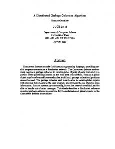
Figure 2: Cases for either early termination, or for the direction of the normal to the linear separator being forced counter-clockwise or clockwise. This early-termination observation is important because it allows B to send to A information regarding a 0-error classifier, with respect to hA , and the points SA that define it. If B cannot terminate, then either some point in DB must be completely misclassified by all separators within the margin, or some negative point in DB and some positive point in DB must both be in the margin and cannot be separated; see Figure 2. Either scenario implies that any "-error classifier on DB must rotate in some direction (either clockwise or counter-clockwise) relative to hA . This is important, because it informs A that all points on @PA (the boundary of PA ) in the clockwise (resp. counter-clockwise) direction from SA will never be misclassified by B if hB rotates in the counterclockwise (resp. clockwise) direction from hA , increasing the SOTA, and decreasing the SOU. This logic is formalized in Lemma 5.1. If the set SA always has half of UA on either side, then this process will terminate in at most O(log(1/")) rounds. But, it may have no points on one side, and always be forced to rotate towards the other side. Thus, the set SA is chosen judiciously to ensure that |UA | decreases by at least half each round.

4.4

Choice of Support Points

What remains to describe is how A chooses a set SA , i.e. how to implement the subroutine Support in Algorithm 1. If the set SA always has half of UA on either side, then this process will terminate in at most O(log(1/")) rounds, via the consequences of no early-termination. But, if no points are on one side of SA , and B’s response always forces hA to rotate towards the other side, then this cannot be assured. Thus, the set SA should be chosen judiciously to ensure that |UA | decreases by at least half each round. We present two methods to choose SA . This first does not have the half-on-either-side guarantee, but is a very simple heuristic, and which we show in Section 7 often works quite well, even in higher dimensions. The second, is only slightly more complicated and is designed precisely to have this half-on-either-side guarantee. Both methods start by computing the region of uncertainty UA and the set of its points DA which lie in that region UA . The first is called MaxMarg, and simply chooses the max-margin support points as SA . These points may include points sent over in previous iterations from B to A. The second is called Median, and is summarized in Algorithm 2 (shown from A’s perspective). It projects all of UA onto @PA (the boundary of PA ); this creates a weight for each edge of @PA , defined by the number of points projected onto it. Then Median chooses the weighted median edge E. Finally, the orientation of hA is set parallel to edge E, and the corresponding support vectors are constructed.

6

Algorithm 2 Support implemented as Median 1: Input: D = DA [ {SB } 2: Output: SA (a set of support points) 3: project points in UA onto @PA ; 4: E := weighted median edge of @PA ; 5: hA := classifier on D parallel to edge E; 6: SA := support points of hA ;

pl

UA

CA pr 5

vl

v

vr

Analysis of IterativeSupports

In this section, we formally prove the number of rounds required by IterativeSupports to converge.

5.1

The Basic Protocol

To simplify the exposition of the protocol, we start with a special case, where player A must, through interaction with B, teach B parameters of classifier that has at most " error on DA , as well as some (but not all) negative examples in DB . This case captures the bulk of the technical development of the overall protocol. In Section 5.3 we will then describe how to extend the protocol to (a) ensure at most " error on both positive and negative examples in DA , and (b) be symmetric: have at most " error on DA [ DB We will describe the protocol from the point of view of player A. Each round of communication will start with A computing a classifier from its current state, and sending support points for this classifier to B. B then performs some computation, and either terminates returning an "-error classifier, or returns a single bit of information to A. A updates its internal state, completing the round. Internal state. At any stage, A maintains an interval of directions (vl , vr ) ⇢ S1 where by convention, we go clockwise from vl to vr . This interval represents A’s current bound on the possible directions normal to an "-optimal classifier based on all conversation with B up to this point. A also maintains CA (recall that CA is the convex hull of the SOTA) as well as the set of points UA that form the SOU . By Lemma 5.2, we know that PA = CA [UA , and therefore there exist a pair of points {pl , pr } on PA whose supporting line segment separates CA and UA . A maintains this pair as well; in fact, vl and vr represent outward normals to PA at pl and pr .

7

+ CA

convex hull rule

pivoting rule

CA (1) A’s move: A projects all points in UA onto the boundary of PA , denoted @PA , (the projection is orthogonal to the edge through {pl , pr }). Each edge in @PA is weighted by how many points are projected to it (with boundary points being assigned arbitrarily to one of the two incident edges). We select the two points on the boundary of edge e which is the weighted median, and place these points in a set S. The normal direction to e is v. And the extreme positive point in DA along direction v is also placed in S. Now the classifier hA is the max-margin separator of S, has 0 error on DA , and is parallel to e. Then A sends (vl , vr , v, S) to B. (2) B’s move: B receives (vl , vr , v, S) from A. It then determines whether there exists a classifier hB with normal v within the margin defined by S that correctly classifies all but an "-fraction of points in B. If so, B sends (hB , 0) to A and terminates, returning hB . Suppose that such a classifier does not exist. Then by Lemma 5.1, any 0-error classifier for DB must have a normal either in the interval (vl , v) or (v, vr ). If the former, B returns (+1) to A, else it returns ( 1). (3) A’s update: If A receives (h, 0) from B, the protocol has terminated, returning h. If A receives (+1), it then updates its interval of directions to be (vl , v) and sets the support pair separating CA and UA to (pl , p). Similarly, if it receives ( 1), it updates the interval of directions to (v, vr ) and sets the support pair to (p, pr ). In both cases, it adds p to CA , updating CA accordingly.

5.2

Structural Analysis

In this section we provide structural results about CA and prove Lemma 5.2 and Lemma 5.1. The first challenge is to reason about the set of total agreement – what points can not be misclassified. Then we can argue that

8

SOTA = CA \ DA . We use two technical tools, the convex hull and a pivoting argument. Let W = union of all Si sent in round i from A to B.

S

i

Si be the

Convex Hull: Let K = C(W ) be the convex hull of all the negative points sent by the protocol so far. No negative points p 2 PA can be misclassified if p 2 K . So K \ PA ⇢ CA . The same rule holds for positive points. Pivoting: Consider any point q 2 PA . If any edge from q to any point p 2 K+ intersects K , then q cannot be misclassified – otherwise a classifier which was correct on p (and incorrect on q) would have to be incorrect on some negative point in K . This identifies another part of PA as being in CA , intuitively the region “behind” K . Note that the early-termination rotation argument, along with this pivoting rule, each round excludes from U all points on one of two sides of the support points in S. We now have the tools to prove the two key structural lemmas needed for our protocol. Lemma 5.1. Consider when B does not terminate. If B returns (+1), then A can update its range to (vl , v). If B returns ( 1), then A can update its range to (v, vr ). Proof. When B can not produce an "-error separator parallel to hA and within the margin provided by S, that implies for any such classifier some points from DB must be misclassified. Furthermore, B can present points Y ⇢ DB that along with S violate any classifier orthogonal to v. Let y, s 2 Y [ S be a negative and positive point, respectively, one of which any classifier orthogonal to v will misclassify. Then any linear separator classifying s and y correctly must intersect the edge between s and y, and thus must rotate from direction v clockwise or counter-clockwise. This excludes directions in either (vl , v) or (v, vr ) and allows B to return (+1) or ( 1), accordingly. Lemma 5.2. After A has updated its state (step (3)), then UA is convex. Proof. First consider the two negative points {pl , pr }. Using the convex hull rule, the edge e12 between them is in CA . And because the points {pl , pr } are defined as the extremal points for the range (vl , vr ) under the pivoting rule, everything “behind” them in PA is also in CA . Thus, CA is partitioned from UA by the line passing through the edge e12 , implying that UA is convex.

5.3

Extending The Basic Protocol

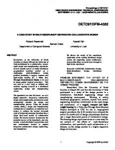
The simplified protocol above captures the spirit of A’s perspective of the algorithm on its negative points. But to show it converges, we need to extend these techniques to also handle positive points and to make it symmetric from B’s perspective. Handling positive and negative instances simultaneously. In each round of the basic protocol UA reduces in cardinality by at least half. We now describe how to modify the protocol so that the entire set UA = UA [ UA+ is reduced in cardinality by half. Recall that in step (1) of the basic protocol, A projects all points in UA to the boundary of PA and determines a edge of the boundary that splits the set in half. In addition now we project all points in UA+ to the boundary of P+ A as well. We can consider the normal direction of each edge in @PA \ U or in + 1 @P+ A \ U and map it to a point on S . We can now scan both sets of normal directions on S1 simultaneously by interleaving the order of directions from + @PA \ U with the antipodal directions from @P+ A \ U . We again find the weighted median direction, corresponding to an edge, now among all negative and positive directions. The set SA now consists of the two points defining the median edge as well as the point incident upon the two edges with normal directions on either side of the antipodal direction of the median edge. As before, this splits the regions of uncertainty into two convex regions on each polytope. The bit returned by B will guarantee that one region on each polytope will be eliminated, and by the above construction, this guarantees that we reduce the size of UA by a factor of two in each round. Lemma 5.3. Over the course of a single round, the size of UA decreases by at least half.

9

v5+ v1

v5+

v4+ v2

v2

v4+

v3+

v3+ v3

v2+

v2+ v3 v4

v1

v4

v1+

S1

v1+

Reducing the SOU for both A and B. The basic protocol and its extension described above only reduce the SOU for A. Since B decides termination, it is possible that the error of the resulting classifier on B never reduces sufficiently. While we could run protocols in parallel for A and B, this could result in classifiers hA and hB that do not have "-error on the entire data set DA [ DB . The solution is for B to send more information back to A. Consider step (2) of the basic protocol. B receives a support set SA from A, as well as the set of directions vl , v, vr and determines which of the intervals (vl , v) and (v, vr ) the direction of a 0-error classifier hB on DB must lie in. Now instead of merely sending back a bit, B also sends back a support set SB corresponding to hB , as well as its own directions (vl0 , vr0 , v 0 ). A now uses the support set SB to update its own SOTA and SOU , completing the round. Notice that now B’s transmission to A in step (2) of the protocol is identical to A’s transmission that initiates step (2)! Thus all future separators proposed by A or B must correctly classify the same set of points in the full protocol transcript.

5.4

Complexity Analysis

Theorem 5.1. The 2-player two-way protocol for linear separators always terminates in at most O(log(1/")) rounds, using at most O(log(1/")) communication. Proof. By Lemma 5.3 we know that as each round shrinks the region of uncertainty SOU by half of its current size for both A and B. And we keep doing this until |UA |  "|DA | or |UB |  "|DB |, then the early-termination condition must be reached. This can be achieved in O(log(1/")) rounds.

6

Multiparty

In the noiseless setting, extending from a two-party protocol to a k-party (where data is distributed to k disjoint nodes) can be achieved by allowing an additional factor k or k 2 communication, depending on the hypothesis class.

6.1

One-way Protocols

For k-players one-way protocols pre-determine an ordering among players P1 < P2 < . . . < Pk , and all communication goes from Pi to Pi+1 for i 2 [1, k 1]. In this section, we show that for k-players, "-error classifiers can be achieved even with this restricted communication pattern. All discussed protocols can also be transformed into hierarchical one-way protocols that may have certain advantages in latency, or where all nodes just send information one-way to a predetermined coordinator node. Sampling results for k-players. In sampling-based player Pi maintains a Si protocols, along the chain of players, Pi random sample Ri of size O((⌫/") log(⌫/")) from j=1 Di and the total size mi = j=1 |Di |. This can be easily 10

achieved with reservoir sampling (Vitter, 1985). The final player Pk computes and returns a 0-error classifier on Rk 1 [ D k . Theorem 6.1. Consider any family of hypothesis (Rd , A) that has VC-dimension ⌫. Then there exists a one-way k-player protocol using O(k(⌫/") log(⌫/")) total communication that achieves "-error, with constant probability. Sk 1 is an "-net, so any 0-error classifier on Rk 1 , is an "-error classifier on j=1 Di . So since Pk 1 the total number of points misclassified is at most j=1 "|Dj |  "|D|, this achieves the proper error bound. The communication cost follows by definition of the protocol. Proof. The final set Rk

1

0-Error protocols for k-players. Any 0-error one-way protocol extends directly from 2-player to k-players. This requires that each player can send exactly the subset of the family of classifiers that permit 0 error to the next player in the sequence. This chain of players only refines this subset, so by our noiseless assumption that there exists some 0-error classifier, the final player can produce a classifier that has 0-error on all data. Theorem 6.2. In the noiseless setting, any one-way two-player 0-error protocol of communication complexity C extended to a one-way k-player 0-error protocol with O(Ck) communication complexity. This implies that k-players can execute a one-way 0-error protocol for axis-aligned rectangles with O(dk) communication. Classifiers from the families of thresholds and intervals follow as special case.

6.2

Two-way Protocols

When not restricted to one-way protocols, we assume all players take turns talking to each other in some preconceived or centrally organized fashion. This fits within standard techniques of organizing communication among many nodes that prevents transmission interference. Linear separators in R2 with k players. Next we consider linear separators in R2 . We proceed in a series of epochs. In each epoch, each player takes one turn as coordinator. On its turn as coordinator, player Pi plays one round of the 2-player protocol with each other player. That is, it sends out its proposed support points, and each other player responds with either early termination or an alternative set of support points, including at least one that “violates” the family of linear separators proposed by the coordinator. The protocol terminates if all non-coordinators agree to terminate early and their proposed family of linear separators all intersect. Note that even if all other players may want to terminate early, they might not agree on a single linear separator along the proposed direction; but by replying with a modified set of support points, they will designate a range, and the manner in which these ranges fail to intersect will indicate to the coordinator a “direction” to turn. Theorem 6.3. In the noiseless setting, k-parties can find an "-error classifier over halfspaces in R2 in O(k 2 log(1/")) communication. Proof. Each epoch requires O(k 2 ) communication; each of k players uses a turn to communicate a constant number of bits with each of k other players. We now just need to argue that the algorithm must terminate in at most O(log(1/")) epochs. We do so by showing that each player decreases its region of uncertainty by at least half for each turn it spends at coordinator, or it succeeds in finding a global separating half space and terminates. If any non-coordinator does not terminate early, it rules out at least half of the coordinator’s points in the region of uncertainty since by Lemma 5.3, the coordinator’s broadcasted support points represent the median of its uncertain points. If all non-coordinators agree on the proposed direction, and return a range of o↵sets that intersect,P then the coordinator terminates the algorithm and can declare victory, since the sum of all error must be at most i "|Di |  "|D| in that range. The difficult part is when all non-coordinators individually want to terminate early, but the range of acceptable o↵sets along the proposed normal direction of the linear separator do not globally intersect. This corresponds to the right-most picture in Figure 2 where the direction is forced clockwise or counter-clockwise because a negative point from one non-coordinator is “above” the positive point from a separate non-coordinator. The combination of these points thus allow the coordinator to prune half of its region of uncertainty just as if a single non-coordinator did not terminate early.

11

7

Experiments

In this section, we present results to empirically demonstrate the correctness and convergence of IterativeSupports. Two-Party Results. For the two-party results, we empirically compare the following methods: (a) Naive- a naive approach that sends all points in A to B and then learns at B, (b) Voting- a simple voting strategy that uses the majority voting rule to combine the predictions of hA and hB on D = DA [ DB ; ties are broken by choosing the label whose prediction has higher confidence, (c) Random- A sends a random sample (an "-net SA of size (d/") log(d/")) of DA to B and B learns on DB [SA , (d) MaxMarg- IterativeSupports that selects informative points heuristically (ref. Section 4), and (e) Median- IterativeSupports that selects informative points with convergence guarantees (ref. Section 4). SVM was used as the underlying classifier for all aforementioned approaches. In all cases, the errors are reported on the dataset D with an " value of 0.05 (where applicable). The above methods have been evaluated on three synthetically generated datasets (Data1, Data2, Data3). For all datasets, both A and B contain 500 data points each (250 positive and 250 negative). Figure 3 pictorially depicts the data.

(a) Data1

(b) Data2

(c) Data3

Figure 3: Red represents A and blue represents B. Positive and negative examples (for all datasets) are denoted by ‘+’s and ‘ ’s, respectively. Table 2 compares the accuracies and communication costs of the aforementioned methods for the dataset in 2-dimensions. For all datasets, MaxMarg and Median required the least amount of communication to learn an optimal classifier. For cases when it is easy to separate the positive from the negative samples (e.g. Data1 and Data2) MaxMarg converges faster than Median. However, Data3 show that there exists difficult datasets where Median requires less communication than MaxMarg. This reinforces our theoretical convergence claims for Median that hold for any input dataset. Data3 in Table 2 shows that there exists cases when both Voting and Random perform worse than Median and with a much higher communication overhead; for Data3, Voting performs as bad as random guessing. Finally, neither Voting nor MaxMarg provide any provable error guarantees.

12

Method Naive Voting Random MaxMarg Median

Data1 Acc Cost 100% 500 100% 500 100% 65 100% 4 100% 6

Data2 Acc Cost 100% 500 100% 500 100% 65 100% 4 100% 6

Data3 Acc Cost 100% 500 50% 500 99.62% 65 100% 12 100% 10

Table 2: Accuracy (Acc) and communication cost (Cost) of di↵erent methods for two-dimensional noiseless datasets. Method Naive Voting Random MaxMarg

Data1 Acc Cost 100% 500 100% 500 100% 100 100% 4

Data2 Acc Cost 100% 500 100% 500 100% 100 100% 4

Data3 Acc Cost 100% 500 81.8% 500 99.1% 100 98.27% 40

Table 3: Accuracy (Acc) and communication cost (Cost) of di↵erent methods for high-dimensional noiseless datasets. Table 3 presents results for Data1, Data2, Data3 extended to dimension = 10. As can be seen, our proposed heuristic MaxMarg outperforms all other baselines in terms communication cost while having comparable accuracies. k-Party Results. The aforementioned methods have been appropriately modified for the multiparty scenario. For Naive, Voting and Random, a node is fixed as the coordinator and the remaining (k 1) nodes send their information to the coordinator node which aggregates all the received information. For MaxMarg and Median, in each epoch, one of the k-players takes a turn to act as the coordinator and updates its state by receiving information from each of the remaining (k 1) nodes. We experiment with a k value of 4 (i.e., four nodes A, B, C, D). As earlier, for all datasets each of A,B,C,D, contain 500 examples (250 positive and 250 negative). The datasets are shown in Figure 4. Method Naive Voting Random MaxMarg Median

Data1 Acc Cost 100% 1500 98.75% 1500 100% 195 97.61% 14 99.0% 36

Data2 Acc Cost 100% 1500 100% 1500 100% 195 100% 2 100% 6

Data3 Acc Cost 100% 1500 50% 1500 99.76% 195 97.38% 38 98.75% 29

Table 4: Accuracy (Acc) and communication cost (Cost) of di↵erent methods for two-dimensional noiseless datasets. As shown in Table 4, for the k-party case, IterativeSupports substantially outperforms the baselines on all datasets. As earlier, for the difficult dataset Data3, Median incurs less communication cost as compared to MaxMarg. We observed that for Data1 and Data2, both MaxMarg and Median require the same number of iterations to converge. However, the cost for Median is higher due to its quadratic dependency on k. One of our future goals is to get rid of an extra k factor and reduce the dependency from quadratic to linear in k (ref. Section 8.2).

8

Discussion

This paper introduces the problem of learning classifiers across distributed data where the communication between datasets is the bottleneck to be optimized. This model focus on real-world communication bottlenecks is increasingly prevalent for massive distributed datasets. In addition, this paper identifies several very general solutions within this framework and introduces new techniques which provide provable exponential improvement by harnessing two-way communication.

13

(a) Data1

(b) Data2

(c) Data3

Figure 4: Red represents A, blue represents B, green represents C and black represents D. Positive and negative examples (for all datasets) are denoted by ‘+’s and ‘ ’s, respectively.

14

8.1

Comparison with Related Approaches

As mentioned earlier, techniques like classifier voting (Bauer & Kohavi, 1999) and mixing (McDonald et al., 2010; Mann et al., 2009) are often used in a distributed setting to obtain global classifiers. Interestingly, we have shown that if the di↵erent classifiers are only allowed to train on mutually exclusive data subsets then there exists specific examples (under the adversarial model) where voting will always yield sub-optimal results. We have presented such examples in Section 7. Additionally, parameter mixing (or averaging (Collins, 2002)), which has been primarily proposed for maximum entropy (MaxEnt) models (Mann et al., 2009) and structured perceptrons (McDonald et al., 2010; Collins, 2002), have shown to admit convergence results but lack any bounds on the communication. Indeed, parameter-mixing for structured perceptrons uses an iterative strategy that performs a large amount of communication. The body of literature that lies closest to our proposed model relates to prior work on label compression bounds (Floyd & Warmuth, 1995; Helmbold & Warmuth, 1995). In the label compression model, both A and B have the same data but only A knows the labels. The goal is to efficiently communicate labels from A to B. Whereas in our model, each player (A and B) have “disjoint labeled” datasets and the goal is to efficiently communicate so as to learn a combined final "-optimal classifier on DA [DB . Indeed some of our one-way results derive bounds similar to the cited work, as they all build on the theory of "-nets. In particular, there exists a label compression method (Helmbold & Warmuth, 1995) based on boosting, which gives O(log 1/") size set for any concept that can be represented as a majority vote over a fixed number of concepts. However, in our model, we show that for certain concept classes (with one-way communication) we need a linear amount of communication (ref. Theorem 3.3). Furthermore, we demonstrate that using a two-way communication model can provide an exponential improvement (ref. Theorem 5.1) in communication cost.

8.2

Future Extentions

Although we have provided many core techniques for designing protocols for minimizing communication in learning classifiers on distributed data, still many intriguing extensions remain. Thus we conclude by outlining three important directions to extend this work and provide outlines of how one might proceed. Higher dimensions. We provide several results for high-dimensions: for axis-aligned rectangles, for bounded VCdimension families of classifiers, and a heuristic for linear separators. But for the most common high-dimensional setting–SVMs computing linear separators on data lifted to a high-dimensional feature space–our results either have polynomial dependence on 1/" or have no guarantees. For this setting, it would be ideal to extend out Median routine which requires O(log 1/") communication in R2 to work in Rd . The key insight required is extending our choice of a median point to higher dimensions. Unfortunately, the natural geometric generalization of a centerpoint does not provide the desired properties, but we are hopeful that a clever analysis of a constant size net or cutting of the space of linear separators will provide the desired bounds. Noisy setting. Most of the results presented in this paper generalize to noisy data. In fact, Theorem 2.1 and Theorem 3.1 have straight-forward extensions to the noisy case by an "-sample argument (Har-peled, 2011). This would increase the communication from O(1/") to about O(1/"2 ). It would of course be better to use communication only logarithmic in 1/". We suggest modifying IterativeSupports to work with noisy data with the following heuristic, and defer any formal analysis. In implementing Support (based either on MaxMarg or Median) we suggest sending over support points of linear separators that allow for classifiers with exactly "-error. That is, players never propose classifiers with 0-error, even if one exists; or at least they provide margins on classifiers allowing "-error. This would seem to describe the proper family of classifiers tolerating "-error of which we seek to find an example. Efficient two-way k-party protocols. All simple one-way protocols we present generalize naturally and efficiently to k-players; that is, with only a factor k increase in communication. In fact, a distributed random sample of size t = O((⌫/") log(⌫/")) can be drawn with only O(t + k) communication (Huang et al., 2011), so under a di↵erent two-way coordinator model some results for the one-way chain model we study could immediately be improved. However, again it would be preferable to achieve protocols for linear separators with communication linear in k and logarithmic in 1/"; our protocols are quadratic in k. In particular, our protocol seems slightly wasteful in that each player is essentially analyzing its improvements independently of improvements obtained by the other players. To improve the quadratic to linear dependence on k, we would need to coordinate this analysis (and potentially the

15

protocol) to show that the joint space of linear separators must decrease by a constant factor for each player’s turn as coordinator, at least in expectation.

9

Acknowledgement

This work was sponsored in part by the NSF grants CCF-0953066 and CCF-0841185 and in part by the DARPA CSSG grant N11AP20022. This work was also partially supported by the sub-award CIF-A-32 to the University of Utah under NSF award 1019343 to CRA. All the authors gratefully acknowledge the support of the grants. Any opinions, findings, and conclusion or recommendation expressed in this material are those of the author(s) and do not necessarily reflect the view of the funding agencies or the U.S. government.

16

Appendix In all cases below we reduce to the indexing problem Kushilevitz & Nisan (1997): Let A have n bits either 0 or 1, and B has an index i 2 [n]. It requires ⌦(n) one-way communication from A to B for B to determine if A’s ith bit is 0 or 1, even allowing a 1/3 probability of failure under randomized algorithms.

A

Lower Bounds for One-Way Linear Separators

Theorem A.1. Using only one-way communication from A to B, it requires ⌦(1/") communication to find an "-error linear classifier in R2 . Proof. We consider linear separators in R2 and suppose that points in DA and DB are distributed (almost) on the perimeter of a circle. This generalizes to higher dimensional settings by restricting points to lie on a 2-dimensional linear subspace. Figure 5 shows a typical example where DA has exactly 1/" negative points around a circle (each lies almost on the circle). These points form 1/2" pairs of points, each close enough to each other and to the circle that they only e↵ect points within the pair. Each pair can have two configurations: • Case 1: left point just inside circle and right point just outside circle (red disks) • Case 2: right point just inside circle and left point just outside circle (red boxes)

h2

h1

- negative points in DA (Case 1) - negative points in DA (Case 2) - positive point (b+) in DB Figure 5: An example to prove the lower bound results for one-way communication with linear separators. The figure on the left shows the distribution of the negative points in DA for case 1 and case 2. The right figure zooms only a small arc of the circle and shows what happens when B decides the final classifier based on its single positive point b+ and all negative points from DA . DB has only one positive point b+ (blue plus) that interacts with exactly one pair of points from DA , but B does not know which pair to interact with ahead of time. The positive point b+ is placed close to the arc of the circle with equal arc length to the negative points from DA on its either sides such that it is just inside the circle. Claim A.1. Let Zj be a pair of points in DA and let xj be the position of b+ (with respect to Zj ), as shown in Figure 5. If DB has a point b+ at xj , then A needs to send at least one bit of information about Zj to B, for B to learn the perfect classifier. Proof. Suppose A sends no information to B. In order to learn an optimal classifier, B makes the classifier tangent to the circle but o↵set to just include its point b+ . However, the point b+ is so positioned that it always forces the

17

classifier learned by B to misclassify either the left negative point in DA (classifier h1 in Figure 5, if case 1) or the right negative point in DA (classifier h2 in Figure 5, if case 2), whichever point is just outside the circle. B can guess case 1 and angle the classifier to the left point, or guess case 2 and angle the classifier to the right point. But in either case, without any information from A, it will be wrong half the time. However, if A sends a single bit of information denoting whether some negative point pair belongs to case 1 or case 2 then B can use this information to learn a perfect separator with zero error. If we increase the number of points to n, by putting "n identical points at each point in the construction then such misclassified points cause an " error. We also note that, each pair of points are independent of the others and a classifier learned for any one negative point pair (in DA ) works for other negative point pairs. In the above case, A has 1/2" point pairs that are all negative. Each pair is far enough away from all other pairs so as not to a↵ect each other. B has 1 positive point placed as shown on the right of Figure 5 for some point pair, not known to A. To reduce this problem to indexing, we let each of A’s point pairs to correspond to one bit which is 0 (if case 1) or 1 (if case 2). And B needs to determine if the ith bit (corresponding to the negative point pair in DA which b+ needs to deal with) is 0 or 1. This requires ⌦(1/") one-way communication from A to B, proving the lemma.

B

Lower Bounds for One-Way Noise Detection

Although in the noiseless non-agnostic setting we can guarantee to find optimal separators with one-way communication, under the assumption they exist, we cannot detect definitively if they do exist. For intervals, the difficult case is when A has only negative points, and for axis-aligned rectangles the difficult case is more general. Lemma B.1. It requires ⌦(|DA |) one-way communication from A to B to determine if there exists a perfect classifier h 2 I. Proof. Consider the case where A has n/2 points and they are all negative. All of its points have values in [2n] and are even. B has 2 positive points and n/2 2 negative, its points have values in [2n + 1] and are all odd. Its two positive points are consecutive odd points, say 2i 1 and 2i + 1. If A has a point at index 2i, then there is no perfect classifier, if it does not, then there is. This is precisely the indexing problem with A’s points corresponding to a 1 if they exist for index 2i and to a 0 if they do not, and for B’s index i corresponding to the value i for which it has positive points at 2i 1 and 2i + 1. Thus, it requires ⌦(|DA |) one-way communication, proving the lemma. Lemma B.2. It requires ⌦(|DA |) one-way communication from A to B to determine if there exists a perfect classifier h 2 R2 , even if A and B have positive and negative points. Proof. Let A and B both have a positive point at (2n, 0) and a negative point at (0, 2n). A also has a set of n/2 2 negative points at locations (2i, 2i) for some distinct values of i 2 [n]. B has a (variable) positive point at some location (2i 1, 2i + 1) for i 2 [n]. There exists a perfect classifier h 2 R2 if and only if A has no point at (2i, 2i) where i is the index of B’s variable point. Again, this is precisely the indexing problem. A’s points along the diagonal correspond to n bits being 1 if a point exists and 0 if not for each index i. And B’s index corresponds to the value i of its variable point. Thus, it requires ⌦(|DA |) one-way communication, proving the lemma.

References http://metaoptimize.com/qa/questions/1885/suppose-your-training-and-test-set-are-generated-by-a-cunningadversary, 2010. Anthony, Martin and Bartlett, Peter L. Neural Network Learning: Theoretical Foundations. Cambridge University Press, New York, NY, USA, 1st edition, 2009. Bauer, Eric and Kohavi, Ron. An empirical comparison of voting classification algorithms: Bagging, boosting, and variants. Machine Learning, 36(1-2), 1999.

18

Bekkerman, Ron, Bilenko, Mikhail, and Langford, John. Scaling up machine learning: Parallel and distributed approaches. www.cs.umass.edu/ ronb/scaling up machine learning.htm, 2011. Cesa-Bianchi, Nicol` o, Gentile, Claudio, and Orabona, Francesco. Robust bounds for classification via selective sampling. In ICML, Montreal, Canada, 2009. Collins, Michael. Discriminative training methods for hidden markov models: theory and experiments with perceptron algorithms. In EMNLP, Stroudsburg, USA, 2002. Dekel, Ofer, Gentile, Claudio, and Sridharan, Karthik. Robust selective sampling from single and multiple teachers. In COLT, Haifa, Israel, 2010. Floyd, Sally and Warmuth, Manfred. Sample compression, learnability, and the vapnik-chervonenkis dimension. Machine Learning, 50:269–304, 1995. Har-peled, Sariel. Geometric Approximation Algorithms. American Mathematical Society, 2011. ISBN 0-8218-4911-5. Helmbold, David P. and Warmuth, Manfred K. On weak learning. Journal of Computer and System Sciences, 50: 551–573, 1995. Hsu, Daniel and Langford, John. The end of the beginning of active learning. http://hunch.net/?p=1800, 2011. Huang, Zengfeng, Yi, Ke, Liu, Yunhao, and Chen, Guihai. Optimal sampling algorithms for frequency estimation in distributed data. In The 30th IEEE International Conference on Computer Communications, 2011. Kearns, Michael and Vazirani, Umesh. An introduction to computational learning theory. MIT Press, Cambridge, MA, USA, 1994. ISBN 0262111934. Kushilevitz, Eyal and Nisan, Noam. Communication Complexity. Cambridge University Press, 1997. Laskov, Pavel and Lippmann, Richard. Machine learning in adversarial environments. Machine Learning, 81(2), 2010. Lazarevic, Aleksandar and Obradovic, Zoran. The distributed boosting algorithm. In KDD, San Francisco, USA, 2001. Mann, Gideon, McDonald, Ryan, Mohri, Mehryar, Silberman, Nathan, and Walker, Dan. Efficient large-scale distributed training of conditional maximum entropy models. In NIPS, Vancouver, Canada, 2009. McDonald, Ryan, Hall, Keith, and Mann, Gideon. Distributed training strategies for the structured perceptron. In NAACL HLT, Los Angeles, California, 2010. Predd, Joel B., Kulkarni, Sanjeev R., and Poor, H. Vincent. Distributed learning in wireless sensor networks. IEEE Signal Processing Magazine, 2006. Settles, Burr. Active learning literature survey. In Computer Sciences Technical Report 1648, University of WisconsinMadison, 2009. Vitter, Je↵rey Scott. Random sampling with a reservoir. ACM Transactions on Mathematical Software, 11:37–57, 1985.

19