1110
J. Opt. Soc. Am. A / Vol. 14, No. 5 / May 1997
Cohn et al.
Fully complex diffractive optics by means of patterned diffuser arrays: encoding concept and implications for fabrication Robert W. Cohn, Anatoly A. Vasiliev, Wenyao Liu,* and David L. Hill Department of Electrical Engineering, University of Louisville, Louisville, Kentucky 40292 Received February 13, 1996; revised manuscript received July 10, 1996; accepted December 11, 1996 Arbitrary complex-valued functions can be implemented as arrays of individually specified diffusers. For any diffuser, only average step height and vertical roughness are needed to control phase and amplitude. This modulation concept suggests potentially low-cost fabrication methods in which desired topographies are patterned by exposing photoresist with partially developed speckle patterns. Analyses and experimental demonstrations that illustrate the modulation concept and aspects of the fabrication method are presented, with particular emphasis on limitations of complex recording set by various photoresist and exposure properties. Applications of diffuser array concepts to spatial light modulators and to gray-scale lithographic printing of micro-optics are also mentioned. © 1997 Optical Society of America [S0740-3232(97)02305-3] Key words: signal synthesis, diffractive optics, computer-generated holography, laser speckle, diffusers, phased arrays, gray-scale lithography, statistical optics.
1. INTRODUCTION The properties of random phase have been widely applied to analyze the scattering of monochromatic light from rough surfaces.1,2 The inverse problem of specifying the statistical properties of phase-only structures so as to obtain desired far-field diffraction patterns has received little attention. Recently, Cohn and Liang introduced a point-oriented encoding method, referred to as pseudorandom phase-only encoding, in which the phase modulation c (x, y) is treated as a nonstationary process in the coordinates x and y. 3 Specifically, the statistics at any point of the modulation are selected so that the statistical average of the random phasor exp( jc) equals the desired fully complex modulation a c exp( jcc) at that same point. The far-field diffraction pattern from this random phase modulation approximates the desired diffraction pattern in the sense of the law of large numbers; that is, as a number of repeated statistical trials, N, is increased, the resulting diffraction pattern more accurately corresponds to its expected value or ensemble average.4 The averaging mechanism here is the superposition in the far field of wave fronts that originate from points across the modulation. To our knowledge, there is no prior art in computergenerated holography in which statistical properties have been varied with position to achieve design objectives. There are many applications in which pseudorandom phase codes are widely used in optical information processing, holography, and optical memory storage; however, these approaches all appear to use pseudorandom phase sequences that are stationary, as opposed to our approach, in which the statistics are nonstationary. Somewhat similar to pseudorandom encoding is the Davis–Cottrell method of randomly multiplexing two (or more) phase-only functions.5 The two individual modulations are randomly interleaved. The probability of se0740-3232/97/0501110-14$10.00
lecting one or the other phase function determines the relative strengths of the individual functions and their diffraction patterns. The random selection is nonetheless a stationary process, and the method does not permit the encoding of arbitrary complex functions. Research on pseudorandom encoding has so far been directed toward real-time programming of spatial light modulators (SLM’s) for pattern recognition filters and toward laser-beam steering and shaping operations.3,6,7 In this study we consider the application of the encoding concept to fixed-pattern diffractive optics. Mathematically, there is no difference between phase-only SLM’s and phase-only diffractive optics, but there are practical differences that suggest entirely new realizations and methods of fabrication. These differences include the following: • The time available to design and fabricate a diffractive optic is much longer than that for real-time programming of SLM’s. • The feature size of diffractive optics (micrometer scale) is usually much smaller than that for SLM pixels (10 to 200 mm), and the spatial bandwidth of diffractive optics is correspondingly larger than that for SLM’s. One implication of increased bandwidth (which is proportional to the number N of independently controllable phase-only pixels) is that the diffraction patterns from pseudorandom encoding will more closely approximate (in the sense of the law of large numbers) the desired diffraction pattern. But there are fabrication costs involved in using the highest resolution. Fine features are typically written point by point with direct-write laser-beam or electron-beam patterning systems. Scanning of laser beams is usually quite slow in order to minimize vibrations.8 Electron-beam scanning can also be slow if there are a large number of mechanical steps between © 1997 Optical Society of America
Cohn et al.
fields. Furthermore, electron-beams are generally expensive to purchase and maintain. These issues have led us to consider a class of design problems in which the desired complex-valued modulation ac [ a c exp( jcc) has a bandwidth that is substantially less than the bandwidth (i.e., the reciprocal of resolution) of the diffractive optic element. When this is true, group-oriented encoding can be used in place of point-oriented encoding.9,10 But, again, group-oriented encoding suggests the need for higher-resolution pattern generators. Perhaps, rather than to direct-write each resolvable point in sequence, a reasonable compromise for this class of diffractive optic design problems is to pattern the entire group in a single processing step. Optical patterning of groups is reasonable given that the system provides an adequate variety of patterns and that the complexity of configuring the patterns is not too great. Furthermore, to justify using such a system in place of current direct-write systems, increased speed and less critical optomechanical tolerances are necessary. In this paper we examine a concept for effectively achieving complex modulation. It is a direct extension of pseudorandom encoding in that any one group is an array of random phase shifts all drawn from the same statistical distribution. We show that each group can be realized as a diffuser pixel having a specified roughness and average step height. We will refer to a diffractive optic composed of an array of custom diffuser pixels as a patterned diffuser array. We describe a fabrication procedure that appears capable of the simplicity, the robustness, and the speed needed to supplant electron-beam and laser writers for fabricating group-oriented designs. Theory, simulations, and demonstration experiments are presented to illustrate the modulation concept and to evaluate the practicality of the proposed patterning procedure. A major emphasis of the evaluation of the patterning procedure is the nonlinear transformation of the random statistics of the exposure pattern (typically, laser speckle patterns) into the desired complex modulation.
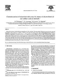
2. CONCEPT: EFFECTIVE COMPLEX MODULATION OF DIFFUSERS AND DIFFUSER ARRAYS The complex-modulating property of diffusers can be appreciated qualitatively by considering the effect of the surface texture of a diffuser on its far-field diffraction pattern (Fig. 1). The diffraction pattern from a smooth surface is a specular intensity pattern. The pattern from a rough surface is a diffuse pattern of noise that is also referred to as a fully developed speckle pattern (only the envelope of diffuse scatter is illustrated in Fig. 1). The grain size of the roughness pattern is typically much smaller than the area of the diffuser that is illuminated; thus the envelope of the speckle pattern is typically much more broadly spread than the specular component. The far-field pattern from a surface of intermediate roughness will contain both specular and diffuse components and is referred to as a partially developed speckle pattern. Thus it is possible to use diffuser surface roughness to attenuate the specular component. The intensity transmittance could be varied from unity to practically zero.
Vol. 14, No. 5 / May 1997 / J. Opt. Soc. Am. A
1111
Fig. 1. Controlling specular intensity by varying surface roughness.
Fig. 2. Array of diffusers that produces a custom complexvalued modulation.
Since the roughness is of a much higher spatial frequency than that of the illumination footprint, the specular component can be much brighter than the diffuse component, even for large values of attenuation. This qualitative description shows the sense in which diffusers control the amplitude of the specular component. Rather than absorbing light with a true attenuator, the unwanted light is scattered into the diffuse component. Of course, the phase can be changed by translating the diffuser along the optical axis. Our approach for encoding complex-valued designs is to use arrays of diffusers, with each diffuser representing a custom value of modulation (as illustrated in Fig. 2). Nearly arbitrary diffraction patterns, limited only by speckle noise, can be produced by superposition in the far field of the specular components from the individual diffuser pixels. A mathematical description of the complexmodulating property of diffusers can be explained in terms of the pseudorandom-encoding algorithm,3 which is reviewed in general terms in this section and then specialized in Section 4 to accommodate the physical constraints set by the fabrication process. This section also compares, by way of example designs, the improvement made possible by using diffuser arrays in place of individual phase-only pixels.
A. Mathematical Description of Effective Complex Modulation and Pseudorandom Encoding The modulation of a plane wave reflected from a phaseonly surface is represented by the complex-valued (indicated by boldface type) function a (x, y) 5 exp@ jc (x, y)#. The far-field diffraction pattern of the modulation pattern is A(f x , f y ) 5 F @ a# , where F [•] is the Fourier transform operator. Since the Fourier transform and the ensemble
1112
J. Opt. Soc. Am. A / Vol. 14, No. 5 / May 1997
Cohn et al.
average are both linear, the average complex-valued farfield pattern of a random modulation can be written as
^ A& 5 F @ ^ a& # ,
(1)
where ^•& is the expectation operator. Under the assumption that the random samples of a are statistically independent of position, the expectation of I, the far-field intensity pattern, is
^ I & 5 ^ u Au 2 & 5 u ^ A& u 2 1 ^ I s & ,
(2)
where I s (f x , f y ) is a residual noise pattern that is due to the random phasings in the far field.3 As long as the noise [represented by the second term of Eq. (2)] is adequately low, then Eq. (2) is approximately the magnitude squared of Eq. (1). Thus the specular and diffuse components of arbitrary diffraction patterns are identified with the two terms in Eq. (2). In the average sense of Eq. (2), any complex-valued modulation can be represented by the random phase-only modulation a (x, y) 5 exp@ jc (x, y)# by using the relationship
^ a& 5
E
p ~ c ! exp~ j c ! dc 5 a p exp~ j f p ! ,
(3)
where p( c ) is the probability density function (pdf) of the phase and a p is the resulting expected amplitude modulation. We will often refer to a p as the effective amplitude, f p as the effective phase, and ap [ (a p , f p ) [ ^ a& as the effective complex amplitude or modulation. The desired modulation ac (x, y) is pseudorandom encoded by specifying a pdf p( c ) in Eq. (3) that gives ap 5 ac . The actual value of phase is selected by using a pseudorandom-number generator that has the required density function. Amplitudes can be encoded by using any number of pdf ’s in Eq. (3). A particularly useful family of pdf ’s is the uniform family of density functions, with spreads n P @ 0, 2p # and phase bias f p 5 c c . These densities, when evaluated in Eq. (3), give all values of amplitude between 0 and 1, according to a p 5 sinc~ n /2p ! .
(4)
Thus the correct density function for encoding a particular value of a p 5 a c is found by inverting Eq. (4) for the appropriate value of n. The most widely available random-number-generator routine is uniform with a spread of 1 and a mean of 1/2. A number selected by this routine would be scaled by n and offset by f p 2 n /2 to produce the actual random phase c. This procedure is applied at every coordinate point to calculate the functions n (x, y) and f p (x, y), which in turn are used to determine the analog phase-only function a(x, y) 5 exp@ jc (x, y)# that represents the desired modulation ac (x, y). Since most of our designs and analyses use discretely sampled functions, we often find it convenient to represent our functions as an array of N samples indexed in i (for example, n i and ai ). Other pdf ’s than the uniform can be used for p( c ) in Eq. (3). In Section 4 our fabrication approaches drive us to consider exponentially distributed (and other) phase statistics. These statistics raise additional challenges in that the phase modulation range of the diffractive optic can be many times larger than 2p for small values of effective amplitude (say, a p 5 0.01 or less).
B. Advantage of Diffuser Pixels over Single-Step Pixels: Directionality Gain Equation (3) describes the effective complex modulation of a phase-only pixel, a diffuser, or arrays of either. Diffusers are typically modeled as arrays of random phases all drawn from the same random distribution. The only mathematical difference between a single pseudorandom phase-only pixel and a diffuser pixel is that the diffuser represents repeated statistical trials of the single pixel. According to the law of large numbers,4 increasing the number of random trials associated with the diffuser pixel will make the far-field diffraction pattern more predictable; i.e., the specular component will be more clearly seen over the noise for diffusers having a larger number of phase samples. This effect can also be interpreted as a directionality gain of the specular component over the diffuse component. If there are N statistically independent roughness samples, or cells, filling an aperture, then the intensity of the diffuse pattern will be reduced by a factor of 1/N over that resulting from one roughness cell filling the aperture. Since the diffraction pattern of the single roughness cell is identical to the pattern of the uniformly illuminated aperture, then the directionality gain of specular to diffuse is N. To demonstrate more clearly the improvement possible by using diffusers in place of single-phase pixels, we compare the performance of encoding a specific complexvalued function into single-phase pixels and into diffuser pixels. The Fourier transform of the complex function produces an 8 3 8 array of equal-intensity spots. A single-phase pixel is modeled as a 3 3 3 array of identical phases, and a diffuser pixel is modeled as a 3 3 3 array of nonidentical phases. Both structures, each an array of 100 3 100 pixels, are pseudorandom encoded by using Eq. (4) to determine the spread n i of the random distribution associated with the ith pixel. The only difference is that for a diffuser pixel there are now nine phases, instead of one phase, selected from the uniform random distribution having spread n i and phase bias f p,i . Another way to describe the difference between the two modulations is that the diffuser array consists of nine spatially multiplexed single-phase pixel encodings, each encoding performed by using a different random seed. The resulting diffracted intensity patterns are shown in Fig. 3. The top row of Fig. 3 shows the diffraction patterns as simulated by using the fast Fourier transform, and the bottom row shows the result for diffraction from a Hughes birefringent liquid-crystal light valve that is programmed to approximate the desired phase modulation. As anticipated, the photographs show that the speckle is more broadly scattered and its intensity is reduced by using diffuser arrays. Numerical measures of the quality of these diffractions patterns are presented in Table 1. The nonuniformity is defined as the standard deviation of the intensity of the 64 spots divided by their average intensity. The signalto-noise ratio is defined as the ratio of the average intensity of the 64 spots to the average background intensity. For the experimental measurements the background intensity is calculated only in the vicinity of the spot array, while for the simulated diffraction pattern the entire pat-
Cohn et al.
Vol. 14, No. 5 / May 1997 / J. Opt. Soc. Am. A
1113
more, applying pseudorandom encoding to nonideal devices produces results that are qualitatively similar to theory. As an additional point of comparison, we have also calculated the performance of encoding the desired complex function aa (x, y) to 300 3 300 single-phase pixels. The complex function is sampled with a higher resolution to 300 3 300 points instead of 100 3 100 points. The nonuniformity, found by simulation, for this single-phase pixel device is 6.8% as compared with 9.9% for the diffuser array. It is not surprising that the performance of the diffuser array is somewhat less than that of the 300 3 300 pixel modulator. However, there is a practical advantage to the diffuser in terms of simplicity of fabrication (described in Section 3). Furthermore, much improved performance is possible by further increasing the resolution of the diffusers. Fig. 3. Comparison of diffraction patterns from random encoding a 100 3 100 array of desired complex values to a 100 3 100 array of phase-only pixels and to a 100 3 100 array of diffuser pixels. Each diffuser pixel is a 3 3 3 array of phases that are randomly encoded to produce the same effective value of amplitude a p . Shown are gray-scale images of diffraction pattern intensity for arrays of (a) phase-only pixels, theory; (b) diffuser pixels, theory; (c) phase-only pixels, experiment; and (d) diffuser pixels, experiment. The on-axis or dc component [upper left of (c) and (d)] is primarily due to Fresnel reflection from the cover glass, which has not been antireflection coated for this liquidcrystal light valve.
Table 1. Measures of Improvement of the Spot Array Design by Using Diffuser Pixels in Place of Single Phase-Only Pixels Nonuniformity (%) Diffuser Resolution Simulation Experiment
Signal-to-Noise Ratio
333
131
333
131
9.9 21.6
23.6 29.4
1639 35
72 14
tern is used. For each measure and for both simulation and experiment, the diffuser array has noticeably better performance. For the experimental intensity patterns, the nonuniformity for the single-phase and diffuser pixel devices was originally measured as 36.9% and 30.4%. However, the images indicate that the intensity gradually decreases with distance from the optical axis. This is due to limited resolution of the SLM (which includes rolloff in the video output of the frame grabber and the cathode-ray tube that is the write light source for the light valve). The values in Table 1 for this experiment report nonuniformity with the linear and quadratic trends in both x and y removed (through the application of a least-squares regression). As further evidence that the rolloff is systematic, the nonuniformity for the theoretical images can be reduced only approximately 2% further (than reported in Table 1) by removing linear and quadratic trends. Even though the experimental spot arrays are less uniform and noisier than theory (because of loss of resolution and inexact phase control of the SLM), the improvements made possible by using diffuser pixels are apparent. Further-
C. Relationship to Prior Kinoform Design Procedures Currently, numerically intensive global search and optimization algorithms are widely used for synthesizing modulation functions under the constraint of phase-only (in many cases binary phase-only) modulation.11–15 Direct pixel-by-pixel or point-by-point encoding can be a practical alternative. Several methods of encoding complex functions onto phase-only diffractive structures were developed shortly after the introduction of the kinoform.9,10 The most direct is the Kirk–Jones method,16 in which a periodic carrier of spatial frequency f 0 that is modulated in amplitude a and phase c a is converted into the phase-only function a~ x, y ! 5 exp@ j c ~ x, y !# 5 exp$ j @ a h ~ 2 p f 0 x ! 1 c a ~ x, y !# % .
(5)
One specific case considered by Kirk and Jones was for h( • ) 5 cos( • ). For this case the Fourier-series expansion of Eq. (5) produces a dc component of complex amplitude ac [ a c exp~ j c c ! 5 J 0 ~ a ! exp~ j c a ! ,
(6)
where J 0 ( a ) is the zero-order Bessel function. Thus ac is proportional to the complex amplitude of the dc or zeroorder far-field diffraction pattern. Any desired value of amplitude a c between 1 and 0 can be implemented by inverting J 0 ( a ) to find the appropriate value of a. Similar results can be developed for h( • ) a square-wave carrier and also for a rectangular carrier of variable duty cycle. From the perspective of the Kirk–Jones approach, patterned diffuser arrays use a random carrier. That is to say, rather than use a single-frequency carrier h( • ), one adopts a carrier that is a randomly phased combination of a continuous range of frequencies. Whereas the traditional Kirk–Jones method scatters unwanted energy into the off-axis harmonics at discrete frequencies, a random carrier scatters unwanted energy uniformly (on average) into a continuous range of frequencies. For the singlefrequency carrier approach, the unwanted harmonics are spatially separated from the desired signal. For the random-carrier approach, the noise and the signal occupy the same space. However, since the noise is spread uni-
1114
J. Opt. Soc. Am. A / Vol. 14, No. 5 / May 1997
formly over the entire observation space, the noise energy is often low enough to ignore. For any of these carrier-based methods, it is important to note that the maximum useful diffraction efficiency of a(x, y) is limited only by the efficiency of the desired complex modulation ac (x, y). Thus there is no implementation loss for the on-axis diffraction order. Furthermore, the optimization of the function ac required to meet a specific set of design criteria is decoupled from the constraints imposed by the phase-only implementation. This could potentially lead to simplified and improved diffractive optic design procedures. (For instance, noniterative optimal window design procedures become possible; see Ref. 3 for a specific design of a top-hat far-field pattern.)
3. MICROTOPOGRAPHIC PATTERNING METHODS A. Comparison with Prior Fabrication Methods Kirk and Jones16 also presented a fabrication procedure in which a photomask having a sinusoidally varying intensity transmittance is placed in contact with a photographic recording medium for which thickness depends linearly on exposure energy. The medium is exposed with an intensity pattern proportional to the function a (x, y). Then the mask is removed, and the medium is further exposed with a second pattern proportional to c a (x, y) 5 c c (x, y) 1 2 p 2 a (x, y) that adjusts thickness to produce the desired phase modulation c c (x, y). [The term 2 p 2 a compensates for the average thickness variations introduced by a h( • ).] If a square-wave carrier is used instead of a sinusoid, the photomask is much easier to produce. If a rectangular carrier is used, the duty cycle is varied. This has the advantage that every pixel can be exposed with the same dose, but it has the disadvantages that the photomask must be written with extreme precision and a custom photomask is needed for each new device design. Also, all three deterministic carriers (sinusoidal, square, and rectangular) require two exposures to produce a desired complex value at a point. A single-exposure method can be envisioned in which laser interference is used to produce sinusoidal fringes and beam balance is adjusted to control phase bias. This pattern would be projected through a small aperture, and the entire photographic medium would be exposed by translating it under the aperture. This method, of course, requires good fringe stability. The Kirk–Jones approach does not seem to have been widely used, apparently because of the requirement for analog control of the exposure. Currently, it is most common to fabricate computer-generated diffractive optic elements as binary and m-ary phase steps. However, lately there has been considerable progress in producing analog phase-only relief structures. Various approaches include projection printing and laser-beam or electron-beam direct write onto photoresist.8,17–20 While the current direct-write systems accurately and precisely write topographic patterns into resist, they also are slow and expensive. As a result of the increasing emphasis on and success of custom-fabricated diffractive optics, we propose an
Cohn et al.
alternative patterning approach; specifically, we consider the possibility of producing patterned diffuser arrays and the technical issues that would affect the quality of the resulting diffraction patterns. B. Proposed Patterning Method Our goal is to develop a robust, repeatable, and easy-toimplement patterning technique. While, in concept, we can write one random phase at a time by direct pseudorandom encoding [Eqs. (3) and (4)], there is really no need for this precise and detailed control. Instead, we can directly use the statistical properties of laser speckle, which are known to be reproducible and controllable. Figure 4(a) illustrates one basic pattern generator concept. This apparatus is a type of proximity printer. An aperture (perhaps patterned on a chrome photomask) having the area of a diffuser pixel is kinematically supported as close to the photoresist as practical. The photoresist is exposed through the aperture, and then the substrate is translated to the next location to be exposed. The high-spatial-frequency random carrier is a fully developed speckle pattern generated by the ground-glass diffuser. An average intensity offset needed to produce a phase bias can be generated by temporal averaging of speckle patterns. This can be achieved, as illustrated in Fig. 4(a), by spinning a ground-glass diffuser with a constant angular velocity. The radial separation between the beam and the diffuser axis determines the linear velocity of the diffuser. Linear velocity together with exposure time then determines the effective bias. A theory for this is described in Section 4. Figure 4(b) shows a modified approach in which a uniform intensity pattern can also be used to provide a phase bias. Statistical properties of the intensities of coherently biased speckle patterns are described in Ref. 1. We specifically consider the case in which the bias and the speckle pattern are mutually incoherent. For the second
Fig. 4. Proximity exposure systems for producing complexvalued pixels. Phase offsets produced by (a) time-averaged recording of speckle patterns from a spinning diffuser and (b) adding a spatially uniform exposure, which, as shown, is derived from a single-mode optical fiber used as a point source.
Cohn et al.
Vol. 14, No. 5 / May 1997 / J. Opt. Soc. Am. A
1115
approach the uniform and speckle illumination could obviously be combined with a beam splitter. However, in order to eliminate beam-splitter loss and multiple reflections, it is possible to bring a uniform coherent illumination through a small aperture (say a fiber optic) in the diffuser, as illustrated in Fig. 4(b). Mutual coherence between the spatially uniform and nonuniform sources can be achieved by rotating a polarized fiber into the cross-polarized state or by using the fiber to introduce a delay difference in excess of the coherence length of the laser. A third approach would be simply to apply appropriate random signals to the exposure control signal on an electron-beam or laser-beam direct-write system. The only advantages of this technique over previous directwritten diffractive optics are that the complexity of the design procedure is simplified and the number of values placed in machine memory can be greatly reduced. C. Alternative Implementations and Applications of Diffuser Arrays We briefly mention two other potential applications of the diffuser array concept. Polymer-dispersed liquid crystal under applied voltage can be converted between isotropic and randomly oriented states. It may be possible to develop a real-time SLM in which this type of liquid-crystal layer is cascaded with pure-phase-retarding pixels. We present this device more as an illustration of the concept of diffuser arrays than as a serious candidate device. The currently prevailing view is that the development of any tandem SLM is too costly and risky. The second application is to use patterned diffuser arrays as gray-scale masks in projection printers. These masks could be used in place of true gray-scale and halftone masks that were recently used to demonstrate projection printing of threedimensional diffractive optical structures in photoresist.17–19 For either the halftone mask or the pseudorandom patterns, grayscale is achieved by diffracting light outside the aperture of the imaging lens. Speckle will not be present in the projected image if the source illumination is adequately incoherent. The grayscale effect can be easily demonstrated by placing a piece of ground glass on the platen of an overhead projector. The pseudorandom masks for projection printing could be fabricated with either system proposed in Fig. 4. The remainder of this paper considers technical issues associated with the patterning systems in Fig. 4.
4. TECHNICAL CONSIDERATIONS FOR PATTERNING DIFFUSER PIXELS IN PHOTORESIST A. Issue 1: Proximity Recording of Laser Speckle Projecting laser speckle through a small aperture may unacceptably blur the exposure pattern. As an example, consider Fig. 5, which shows how a fully developed speckle pattern (457-nm argon-ion wavelength) diffracts at various distances past a 100-mm slit. At a distance of 100 mm past the slit, the edges of the pattern are still rather sharp, showing a transition from light to dark on the order of 10 mm. This indicates that pixels having a large fill factor can be made by proximity exposure for
Fig. 5. Gray-scale intensity images of speckle patterns recorded at (a) 0 mm, (b) 100 mm, and (c) 500 mm past a 100-mm slit. The diameter of the speckle is approximately 2.5 mm. Patterns were imaged onto a 1/3-in. (0.85-cm) CCD camera by using a 403 microscope objective approximately 160 mm from the CCD. The images were then recorded with a video frame grabber.
reasonable (10–100-mm) separations between mask and resist. It is even feasible to maintain separations of less than 10 mm, but at minute distances there would be little further reduction in the shadow region on account of the resist thickness, which may be exposed to a depth of several micrometers (described in Subsections 4.B–4.G). As compared with recording interference fringes, speckle requires minimal vibration isolation. For a diffuser, a laser, and a CCD observation camera on a 2-in.(5.08-cm-) thick optical bread board supported by a wood table, we observed that speckle patterns displayed on a video monitor exhibited no apparent displacement for speckle diameters larger than 2 mm. Vibration was noticeable for 0.6-mm speckle, but no blurring was observed for 1/30-s exposure frames recorded by using a frame grabber. Thus it seems that it is quite practical to illuminate resist with 2-mm speckle through an aperture in near contact (100 mm or less). For pixels of the order of the size of current SLM pixels (12.5–100 mm), the directivity gains can be 39 to 2500. B. Issue 2: Complex Modulation for Recording Speckle in Linear Resist The pdf of I s , the intensity of fully developed speckle, is known to be exponentially distributed1,2 and is written as p~ Is! 5
1
^ I s&
exp
S D 2I s
^ I s&
,
(7)
where ^ I s & is the average intensity of the speckle pattern. Also, since speckle intensity is exponentially distributed, ^ I s & can be interpreted as the standard deviation of the
1116
J. Opt. Soc. Am. A / Vol. 14, No. 5 / May 1997
Cohn et al.
speckle intensity. For a photoresist that linearly maps exposure energy into resist thickness, c s , the random phase depth produced, is proportional to exposure energy E s and intensity I s of the speckle pattern. Likewise, a mutually incoherent and spatially uniform illumination can be used to produce a bias phase shift c b , so that the total random phase shift can be expressed as c 5 c b 1 c s , where c b is proportional to E b , the bias exposure. The effective complex modulation produced by this surface can be found by treating the actual phase depth c as an exponentially distributed random variable. Using the pdf for c of the form of Eq. (7) in Eq. (3) yields
^ a& 5
exp@ j ~ c b 1 arctan^ c s & !#
A1 1 ^ c s & 2
.
(8)
The amplitude decreases monotonically with increasing average phase depth of the resist, ^ c s & (which is also proportional to average energy density of the speckle, ^ E s & ). The phase shift that is due to speckle alone varies only from zero to p /2, but c b can be chosen to produce any phase shift from zero to 2p. C. Issue 3: Selecting Resist Thickness to Ensure Linearity A linear resist will effectively saturate if developed through its entire thickness down to the substrate. This nonlinearity will change the complex modulation over that predicted by Eq. (8). Consider that the total resist thickness is proportional to the maximum phase shift c m 5 c b 1 c ms , where c ms is the maximum phase shift available for speckle recording at a given bias. The effective complex modulation for this case is found by evaluating Eq. (3) as
^ a& 5 exp~ j c b !
FE
c ms
p ~ c ! exp~ j c ! dc
0
1 exp~ j c ms !
E
`
c ms
G
p ~ c ! dc ,
(9)
where the density function is of the exponential form in Eq. (7). This evaluates to
^ a& 8 5
exp@ j ~ c b 1 arctan^ c s & !#
3
H
A1 1 ^ c s & 2 1 1 ^ c s & exp@ j ~ c ms 2 p /2!# exp
S DJ 2c ms
^ c s&
,
(10) where the prime is used to indicate that this result is perturbed from the result in Eq. (8). If the saturated value of phase c ms is much greater than ^ c s & , the average phase produced by a purely linear recording of speckle, then Eq. (10) reduces to Eq. (8). Thus the second term in braces in Eq. (10) represents the errors that are due to finite resist thickness. A minimum thickness can be selected based on the minimum amplitude a min of a c P @ a min, 1# that is practical to implement and the maximum allowable error e between Eqs. (8) and (10). The worst-case absolute error is approximately
e ~ a c ! ' exp~ 2a c c ms ! ,
(11)
where the approximation a c 5 u ^ a& u ' 1/^ c s & for average phase depth much greater than 1 rad has been used in Eq. (10). The minimum total resist thickness is then proportional to
c t [ c mb 1 c ms 5 2 p 2 ~ ln e min! /a min ,
(12)
where e min 5 e (amin) and c mb 5 2 p is the maximum bias shift required to achieve all possible phase shifts. Using c ms as defined in Eq. (12) in relation (11) gives error as a function of a c of
e ~ a c ! 5 ~ e min! a c /a min.
(13)
As a specific example of using these equations to select resist thickness, consider the case for a minimum amplitude of a min 5 0.025 and an absolute error of e min 5 0.0025, or a 10% relative error. With the use of Eq. (12), the resist thickness is c t 5 246 rad or 39.1 optical wavelengths. For a reflective surface relief pattern and an optical wavelength of 0.633 mm, the resist can be as thin as 12.3 mm. Equation (13) shows that the relative error decreases rapidly for a c . 0.025. For example, for a c 5 0.03 the error drops to 0.00075. Resist thickness is then only a significant concern for very small amplitudes, i.e., those values smaller than 0.025. The thickness is quite reasonable for standard photoresists.20,21 For comparison, the Kirk–Jones method using a sinusoidal carrier requires a thickness of at least
c t 5 2 p 1 2J 0 21 ~ a min! ,
(14)
which follows from Eqs. (5) and (6). For a min 5 0 the total thickness for a reflective surface is 0.56 mm. While the thickness of the resist for the random method is much larger than that for the deterministic method, it should be recognized that the selection of thickness in relation (11) and Eq. (12) used a worst-case design. Furthermore, the maximum average speckle exposure energy is proportional to ^ c s & ' 1/a min , which corresponds to an average depth of 2 mm. Thus the comparison in terms of energy use is more favorable. The basic conclusion for these numerical examples, is that the resist can be treated as infinitely thick for resists six times thicker than the average speckle depth. The pseudorandom method can also produce an effective zero. If the magnitude of the second term in braces in Eq. (10) is unity and c ms 5 c t 2 c b and ^ c s & are chosen to produce a phase shift of p, then Eq. (10) is zero. This is equivalent to having a relative error of 100% between Eqs. (8) and (10). For example, for the 39.1wavelength-thick resist discussed above, an exposure depth of 9.6 wavelengths or 3.05 mm produces a zero according to Eq. (10) as compared with an amplitude of a c 5 0.0165 for an infinitely thick resist [according to Eq. (8)]. Unless the exposure system is precisely controlled and the resist thickness is precisely known, it would actually be quite difficult to implement a true zero accurately by this method. In most applications a very low minimum effective amplitude should be adequate.
Cohn et al.
Vol. 14, No. 5 / May 1997 / J. Opt. Soc. Am. A
D. Issue 4: Transformation of Speckle Statistics by Recording in Log Nonlinear Resist For many resists, thickness is proportional to the logarithm of exposure over a wide dynamic range. For such resists the exposure curve (depth into the resist, t, versus exposure energy E) takes the form t ~ E ! 5 m ln~ E/E b ! ,
(15)
where E b is a reference recording level corresponding to a reference thickness of t 5 0 and m is the logarithmic slope of the resist. The exposure curve of a 9.5-mm-thick film of resist (AZ 4903 positive) presented in Ref. 16 is well fit over a 7-mm range for a slope of m 5 2.70 mm and a reference energy of E b 5 75 mJ/cm2. For 5-mm films of Shipley S1650 resist, we have experimentally determined that the slope is m 5 0.823 mm over a 2.6-mm range starting from a reference energy of E b 5 40 mJ/cm2. Using the logarithmic range of a resist leads to an effective amplitude that depends on the ratio of speckle exposure to bias exposure rather than absolute intensity. This may prove to be an advantageous feature, since it is often easier to control ratios (using a half-wave plate and a polarized beam splitter) than it is to control the absolute energy individually in two independent exposures. The effective amplitude can be found by using the following analysis. The logarithmic recording medium produces the total phase shift
c t 5 c b 1 c s 5 a ln~ E s 1 E b ! ,
(16)
where a is the logarithmic slope in radians (i.e., a 5 4 p m/l for a reflective surface) and c b 5 a ln (Eb). This definition allows the phase shift that is due to speckle to be written as
c s 5 a ln~ 1 1 E s /E b ! .
(17)
Using the definitions in Eqs. (15) and (16), the exponential density of the form of Eq. (7), and the change of variables x 5 E s / ^ E s & in Eq. (3) leads to
^ a& 5 exp~ j c b !
E
`
exp~ 2x ! exp@ j a ln~ 1 1 g x !# dx
0
5 exp@ j ~ c b 1 a ln g !# exp~ 1/g ! G ~ 1 1 j a , 1/ g ! ,
1117
5 a ln(1 1 Ems /Eb), where E ms is the amount of energy above bias at which the resist is completely exposed. With these definitions the perturbed version of Eq. (18) is written as
^ a& 8 5 ^ a& 1 e
H S
5 ^ a& 1 exp~ j c b ! exp 2
E
`
g ms / g
2g ms 1 j c ms g
D
J
exp@ 2x 1 j a ln~ 1 1 g x !# dx ,
(19)
where the definition g ms 5 E ms /E b has been used and e is the absolute error resulting from the perturbation. Continuing with the numerical example begun in Subsection 4.C, a value of g is found, by using Eq. (18), for which a c 5 0.025. For the resist with the smaller logarithmic slope ( a 5 16.34), a value of g 5 2.45 is needed to produce this amplitude. For the resist with the larger slope, a value of g 5 0.745 is needed. For an absolute error e , 0.0025, then, the ratio g ms / g 5 E ms / ^ E s & needs to be approximately 6 or greater [as found by numerical evaluation of Eq. (19)]. This is essentially identical to the result for linear photoresist. However, on account of the nature of the logarithmic resists, the resist thickness can be much less than that for linear resists. The minimum thicknesses are 2.26 mm for the low-a resist and 4.59 mm for the high-a resist, as compared with 12.1 mm for the linear resist. The required thickness can be appreciated by comparing it with the pdf for the recorded depths (which are proportional to the random phases c s ). This is shown in Fig. 7. The density function for logarithmically recorded speckle has been derived by a standard technique for transformations of random variables.4 This function is written as p~ cs! 5
H
F
S D GJ
cs cs 1 1 exp 1 1 2 exp ag a g g
.
(20)
Note that for each curve in Fig. 7, p(0) 5 0.025 5 a c . Also note that for the logarithmic resists, p(0) 5 1/( ag ). The relationship between the pdf and the effective ampli-
(18) where g 5 ^ E s & /E b and G(a, b) is the incomplete gamma function.22 Figure 6 shows the effective amplitude produced by exposing the S1650 and AZ4903 resists (described above) with speckle patterns and then reflecting 633-nm light from the resulting surfaces. This corresponds to using a 5 16.34 and 53.6 in the evaluation of Eq. (18). For these values of a, the effective phase (excluding bias c b ) varies by slightly more than p/2 for all values of g. This amount of phase modulation is comparable with the maximum phase shift for linear resists [see Eq. (8) and Fig. 6]. The minimum resist thickness that effectively behaves as infinitely thick [thus permitting the use of Eq. (18)] can be determined by an analysis similar to that in Subsection 4.C. The maximum phase shift for which the resist is exposed down to the substrate is once again written as c m 5 c b 1 c ms . However, the maximum phase shift that is due to speckle is now explicitly written as c ms
Fig. 6. Effective amplitude a p and phase f p for log and linear resists. For linear resist, which depends on absolute intensity, the x axis is defined to be g 5 ^ c s & / p .
1118
J. Opt. Soc. Am. A / Vol. 14, No. 5 / May 1997
Cohn et al.
tude is approximately valid for a > 4. For a near 5 the pdf curve is even more sharply peaked and narrower than that for the a 5 16.34 curve, and the maximum resist thickness is approximately 1 mm. For a . 53.6 the pdf more closely approaches the exponential distribution for a linear resist. For an appropriately chosen value of a, a logarithmic transformation of speckle permits the use of much thinner films than those for linear resists. E. Issue 5: Special Case: Low-Sensitivity Log Resist For resists having sensitivities below 4, the effective amplitude cannot be continuously controlled between one and zero. This can be seen by evaluating Eq. (18). For large values of g, the effective amplitude is well approximated as
^ a& ' exp@ j ~ c b 1 a ln g !# G ~ 1 1 j a ! ,
(18a)
where G( • ) [ G( • , 0) is the gamma function. The magnitude of relation (18a) decreases monotonically with increasing a. For example, for a p 5 0.01, 0.25, 0.5, and 0.75, a 5 4, 1.62, 1.04, and 0.625, respectively. The effective amplitude as a function of g [as calculated by using Eq. (18)] can oscillate around the limiting value of effective amplitude, but this is usually a negligible amount. The only significant undershoot is evident for a close to a 5 2.72. In this instance the effective amplitude as a function of g dips to zero (at g . 5) before settling to an effective amplitude of 0.058. The most important point is that a high-contrast material ( a . 4) is required in order to produce fully complex modulation. F. Issue 6: Time-Averaged Recording in Linear Resists The patterning system in Fig. 4(a) uses time averaging of speckle patterns (achieved by varying the velocity of the spinning diffuser) to control both effective amplitude and step height. The effect of time averaging of speckle patterns is reasonably modeled as the addition of M equalintensity exposures of uncorrelated speckle patterns in sequence (Ref. 1, Chap. 4). With exposure time and exposure energy held constant, the parameter M is proportional to the velocity of the diffuser. Alternatively, with velocity held constant, M is proportional to exposure time. Except for values of M close to unity, the resulting curves for effective amplitude can be accurately interpolated for continuous values of M. 1 Here we model time-
Fig. 7. Probability density functions for depths of speckle recorded into log and linear resists. Each distribution produces effective amplitude a p 5 0.025.
Fig. 8. Effective complex amplitude for time-averaged recording of speckle in linear resist. Average recorded depth is proportional to average exposure energy ^ E s & . The amplitude and phase curves use the same style for a given value of M. For M of 80, 180, and 602, the effective phase curves are nearly identical and, for this reason, are plotted with a single style. The dots (d) indicate where effective phase is 2.5p.
averaged complex recording in linear resist. Then, in Subsection 4.G we consider time averaging in nonlinear resist. The pdf for each exposure is Eq. (7), and the pdf for the total exposure is the result of convolving the M identical pdf ’s.4 The pdf for the phase c s that is due to this total exposure is the gamma density1 p~ cs! 5
S D S
c s M21 M G ~ M ! ^ c s&
D
Mcs , ^ c s&
M
exp 2
(21)
where ^ c s & /M is proportional to the exposure energy of an individual speckle pattern. The effective complex amplitude is known to be the characteristic function of the pdf evaluated at frequency equal to unity,2 and thus the complex amplitude is of the form of the Mth power of Eq. (8):
F S DG
^ a& 5 1 1
^ c s& M
2 2M/2
FS
exp j M arctan
^ c s& M
DG
. (22)
The effective amplitudes and phases of Eq. (22) are plotted in Fig. 8 against average exposure and for various values of M. The dots on the curves indicate specific points for which the effective phase shift is 2.5p. For the dot markers the amplitude varies between 0.031 and 0.95 for M between 10 and 602. [For M 5 1 the results are the same as those with Eq. (8).] Near-unity amplitudes can be produced, but not for all values of phase. It may not be practical to increase M further, as this increases recording time. One way to address this wide variation in M is to control multiple parameters such as intensity, diffuser angular velocity, and radial position of the laser beam on the diffuser. This would allow a modest range of control (less than 10:1) on each of the three parameters. It may also be desirable to add a separate phase bias c b for amplitudes that are close to unity in order to reduce recording time. The principal advantage of time-averaged recording is that the maximum recording depth is substantially less
Cohn et al.
Vol. 14, No. 5 / May 1997 / J. Opt. Soc. Am. A
1119
than that for nonaveraged recording. This is shown in Fig. 9 for the density functions corresponding to M 5 2, 10, and 29 and effective amplitude a p 5 0.025. The effective values of phase shift are, respectively, 0.9p, 2.6p, and 4.6p. These curves can be compared with Fig. 7. They are substantially narrower than the exponential density. The curves for M 5 1 to 10 and M 5 10 to 29 both produce a 2p range; however, the second set of curves (compare M 5 2 with M 5 29) are even narrower. Also, the exposure energy used for time-averaged recording will be smaller by a factor of 2 to 4. This can be seen by inverting the amplitude in Eq. (22) for average exposure energy:
^ E s & } ^ c s & 5 M Aa p 22/M 2 1.
(23)
For a p 5 0.025 and M 5 1, which corresponds to the exponential distribution, the average intensity is proportional to 12.7p. For M 5 2 the exposure drops to 4.0p. For M 5 5 the energy is minimum at 2.9p, and it increases gradually to 5.0p at M 5 29. Therefore both exposure energy and film thickness can be much less if temporal averaging is used. For monochromatic diffractive optic design, phase modulations f p that differ by integer multiples of 2p are often treated as equivalent. This 2p phase ambiguity can be used to produce the same effective value of the complex modulation ac 5 (a c , c c ) for different exposure conditions. A particular choice of exposure conditions may be preferable from various considerations of energy efficiency, accuracy, and recording time. We illustrate this by expressing the amplitude a p in terms of the phase f p in Eq. (22). The term ^ c s & /M that is in common between the expressions for amplitude and phase is substituted out to give a p 5 u cos~ f p /M ! u M .
(24)
Figure 10 plots both the desired amplitude [Eq. (24)] and
^ C s & (which is proportional to average exposure energy) against M (which is proportional to the amount of time averaging). The three curve styles are used to distinguish the results for three effective values of phase f p that differ from each other by integer factors of 2p (specifically, p /2, 5 p /2, and 9 p /2). The solutions represented by dots in Fig. 8 (for M 5 10, 80, and 180) are replotted in Fig. 10 (again shown as dots). These values were calculated for f p 5 5 p /2 and thus are located on the solid curves. For each of these solutions, there is an alternative recording condition that produces the same complex amplitude (indicated in Fig. 10 by diamonds).
Fig. 10. Effective amplitude for time-averaged recording in linear resist for a constant value of effective phase. The dots (d) indicate identical points from Fig. 8. The diamonds (l) indicate points identical in amplitude but differing in phase by an integer multiple of 2p.
We can see that one recording condition may be preferred to another. For instance, for the smallest effective amplitude (a p 5 0.031) the solution on the 9 p /2 curve uses more energy than that for the 5 p /2 curve, but the amplitude is less sensitive to exposure time. For the two larger-amplitude solutions, the alternative choices on the p /2 curve use less energy but are much more sensitive to exposure time. Figure 8 also shows that the sensitivity of the amplitude with respect to exposure energy generally decreases with increasing exposure energy. For large amounts of time averaging, Eq. (22), the effective amplitude, can be simplified. The gamma density function in Eq. (21) can be approximated as a Gaussian of the form p~ cs! '
F S
1
A2 p M ^ c s &
exp
1
c s 2 ^ c s&
2M
^ c s&
DG 2
.
(21a)
for M a large number, through the use of the central limit theorem (see Ref. 4, pp. 214–221 and 240). Substituting this result in Eq. (3) approximates the effective amplitude of Eq. (22) as
^ a& ' exp~ j ^ c s & ! exp
S
D
2^ c s & 2 . 2M
(22a)
This result is quite good for M . 10. This result accurately describes the effective amplitude and phase for M 5 80, 180, and 602. In particular, note that the effective phase f p is independent of M. This can be seen in Fig. 8, where the effective phase curves (and also the three dots at ^ c s & 5 2.5p ) are all nearly identical. G. Issue 7: Time-averaged Recording in Log Resist The analysis of effective amplitude is identical to that used in deriving Eq. (18), except that the gamma density is used in place of the exponential density. This gives
^ a& 5 exp~ j c b !
E
`
0
F S
x M21 exp~ 2x ! G~ M !
3 exp j a ln 1 1 Fig. 9. Probability density functions (pdf ’s) for time-averaged recording in linear resist. Each pdf produces identical effective amplitude a P 5 0.025.
gx M
DG
dx.
(25)
The amplitude again depends on the ratio of speckle intensity to bias intensity. For M 5 1 Eq. (25) is identi-
1120
J. Opt. Soc. Am. A / Vol. 14, No. 5 / May 1997
Cohn et al.
cally Eq. (18). For any value of M, the amplitude decreases monotonically with increasing g. For M a large number, the gamma density in Eq. (25) can be replaced by its approximate form [relation (21a)]. After an appropriate change of variables, Eq. (25) is approximated as
^ a& '
exp~ j c b !
A2 p
E
`
2`
exp~ 2x 2 /2!
3 exp@ j a ln~ 1 1 g 1 g x/ AM !# dx.
(25a)
Factoring out the term 1 1 g in the log function and using the approximation ln(1 1 z) ' z for values of z , 1, we can further simplify Eq. (25) to
F S
^ a& ' exp@ j c b 1 j a ln~ 1 1 g !# exp
21 ag 2M 1 1 g
DG 2
.
(25b) The range of validity of the expansion depends on the extent of the Gaussian in relation (25a). The Gaussian is essentially zero for x . 3. This leads to M . 9 @ g /(1 1 g ) # 2 , which is always true for M . 9. Relation (25b) shows that the effective amplitude a p monotonically decreases with increasing speckle-to-bias ratio g. For low-sensitivity resist (see Subsection 4.E), the curves saturate without reaching zero. Increasing M raises only the saturation value and does not increase depth of amplitude modulation over recording without time averaging. The amplitude control provided by time averaging in log photoresist is similar to that for timeaveraged recording in linear resists, as can be seen by comparing relations (22a) and (25b). The main difference between the two results is that relation (22a) always approaches zero given a large enough exposure, while relation (25b) instead settles to a constant amplitude determined by a 2 /M. H. Issue 8: Spatial Resolution of Linear and Log Resists Photoresists generally have much higher spatial resolution than the diffraction limit. However, if speckle is reimaged through a projection system, it would be possible to use an adjustable iris in place of the spinning diffuser. The blurred speckle pattern can then be considered as spatially integrated. The problem is analyzed in Chap. 2 of Ref. 1, and it is not surprising that the results are identical to the analysis of time-integrated speckle given above. As above, the gamma function is a good approximation of the pdf of the spatially averaged speckle intensities. The parameter M is now interpreted as the effective number of speckles averaged together in a rectangular window. Thus the results presented above in Subsections 4.F and 4.G can be used without modification to analyze the effect of resolution loss in linear and logarithmic resists.
5. EXPERIMENTAL DEMONSTRATION OF SPECKLE RECORDING The theory presented in Section 4 primarily describes the complex amplitudes that could be produced by recording laser speckle in photoresist. In order to anticipate better the potential problems in developing the proposed expo-
sure system, we have also performed some preliminary experiments in which we use a phase-only liquid-crystal light valve to represent photoresist. Unlike the demonstration reported in Section 2, in which the SLM represented an array of pixels, in this section the SLM represents a single pixel. One purpose of the demonstration is to show experimentally the control of effective amplitude by varying the exposure patterns. In one set of measurements, the exposure energies of speckle, ^ E s & , and of bias, E b , are varied. This corresponds to exposure using the apparatus in Fig. 4(b). In a second set of measurements, the speckle energy and the speckle diameter are varied. The SLM has limited spatial resolution, so the SLM introduces spatial averaging. As pointed out in Subsection 4.H, spatial averaging gives results that are mathematically equivalent to time averaging. Thus this second set of measurements is representative of results made possible by using the patterning system in Fig. 4(a). The second purpose of the demonstration is to relate the experimental measurements to our theory of speckle recording. However, the optical characteristics of SLM’s that we have studied are much more complicated than the properties assumed for resists. The SLM used for this demonstration is a gallium arsenide photodetector, birefringent liquid-crystal light valve from the Lebedev Physical Institute, Moscow. It was chosen because it produces the largest phase shift (up to 4 p) of the SLM’s available to us. Measurements in a Michelson interferometer of the read side of the light valve indicate that there is a roughly logarithmic dependence of the phase modulation depth on the exposure intensity. However, the exact phase shifts measured can vary dramatically based on the spatial-frequency content of the illumination and the exposure intensity. In particular, the spatial resolution of the device (4 to 40 line pairs per millimeter) is known to depend on the exposure intensity. Rather than attempting to measure and then model the SLM completely, we have attempted empirically to fit theoretical curves for a logarithmic film of resist to the measured response of the SLM. This is to say that it has been possible to adjust parameters (specifically, a, E b , c ms , and M) in the theoretical equations so that the trends in the experiment match the theory. This exercise is certainly valuable for better appreciating the theory and for anticipating the practical limitations of actual photoresists. We also believe that the process of comparison of the experiment with an approximate theory provides insight into the optical characteristics of the SLM.
A. Measurement Procedure The effective amplitude is measured by using the following procedure. The write side of the light valve is illuminated by two mutually incoherent (850-nm) laser diode sources. One beam is expanded and illuminates the light valve with a spatially uniform bias. The other beam is focused into a small spot on the surface of a ground-glass diffuser to produce a speckle pattern illumination on the light valve. The speckle diameter is varied by translating a diffuser along the path of the beam so as to change the beam diameter intercepting the diffuser. The light
Cohn et al.
valve is electrically driven with a 2-kHz, 10-V rms sinusoidal potential from a signal generator. The read side of the light valve is illuminated with a 633-nm-wavelength HeNe laser beam. The beam is spatially filtered and expanded by using a collimator. The collimator lens is positioned to converge the beam slightly. At the face of the SLM, the beam is 14.5 mm in diameter. The reflected beam is observed by using a CCD camera positioned at the focus of the collimator lens. A digital oscilloscope connected to the video output of the camera is used to measure the intensity of the specular diffraction peak for a range of speckle exposure (0 – 365 m W/cm2) and different settings of bias exposure (0, 9.8, 15.3, and 29.3 m W/cm2) or speckle diameter (0.07, 0.15, 0.25, 0.4, 1, and 3 mm). The measured intensities are normalized so that the SLM has nominally unity transmittance for zero intensity exposure. The measured effective amplitude a p is taken to be the square root of the normalized intensity. These results are plotted in Fig. 11. The results for speckle recording at different levels of bias [Fig. 11(a)] and for various speckle diameters [Fig. 11(b)] are discussed in sequence. B. Complex Recording by Combined Speckle and Bias Exposure As discussed in Subsection 4.D, for an ideal logarithmic resist of infinite thickness, Eq. (18) shows that the ratio of speckle energy to bias energy, g 5 ^ E s & /E b , determines the effective amplitude and that the bias energy can be used to offset the effective phase by c b 5 a ln (Eb). This result becomes complicated for resists for which the exposed depth approaches the film thickness, as modeled by Eq. (19). For a thin film the total phase modulation range is c m 5 c b 1 c ms , where c ms is the phase modulation range available in the resist for speckle exposure. If c ms is too small, then the effective amplitude cannot be varied from unity to zero. Thus, for a fixed thickness film, the amplitude range should decrease as the bias is increased. We will refer to this effect as saturation of the effective amplitude. This saturation is observed for the measured curves in Fig. 11(a). For each curve the amplitude decreases with increasing speckle level to a point and then begins increasing. As the bias level (listed in Table 2) is increased, the minimum amplitude increases correspondingly. The bias levels have been selected so as to produce phase shifts c b (these values, which were measured in the Michelson interferometer, are listed in Table 2) covering a 2p range. Thus this SLM, while it can control amplitude over a 10:1 range, cannot simultaneously produce all values of phase. Basically, the SLM needs more (than its current 4p) phase modulation range to achieve arbitrary phase and a 10:1 amplitude control. For an ideal logarithmic resist, the effective amplitude is governed by Eq. (18) for low combined levels of speckle and bias exposure. Thus plots of effective amplitudes versus speckle-to-bias ratio g will appear identical for low-level exposures. For the measured curves in Fig. 11(a), the initial slopes differ if the measured values of E b are used. In order to compare the measurements for the SLM with the theory for an ideal resist, values of E b (listed in the ‘‘E b theory’’ column in Table 2) are used to
Vol. 14, No. 5 / May 1997 / J. Opt. Soc. Am. A
1121
Fig. 11. Experimental demonstration of speckle recording using a phase-only liquid-crystal light valve to represent a photoresist. The plots show how the effective amplitude curves change for (a) different levels of uniform bias E b and (b) different speckle diameters. Specific values used in the experiment and the theory are given in Tables 2 and 3.
Table 2. Parameters Used for the Measured and Theoretical Curves in Fig. 11(a) E b ( mW/cm2)
c b (rad)
Curve ID
Measureda
Theoryb
Measureda
Theoryb
1 2 3 4
29.3 15.3 9.8 0.0
12.3 15.3 9.8 5.1
2.0p 1.5p 1.0p 0.0p
0.91p 1.26p 1.67p 2.06p
a b
Measured speckle diameter is 1 mm. Theoretical value of a is 1.65 rad.
calculate g for the measured curves in Fig. 11(a). With these choices of E b , the initial slopes of curves 1 and 4 are brought into coincidence with curves 2 and 3 (which are plotted by using the measured values of E b ). With these adjustments it is possible to compare the experimental results with the theory for logarithmic resist. The theoretical curves in Fig. 11(a) are calculated by using Eq. (19). The value of logarithmic slope a 5 1.65 has been selected so that the initial slopes of theoretical and measured curves match. Then values of c ms (the phase modulation range available for speckle recording, which is listed in Table 2) are selected to introduce the saturation effect near the minima of the measured curves. The minima of theoretical curve 4 cannot be brought much lower for any value of c ms unless the sensitivity a is also increased, as described in Subsection 4.E. [A fit to curve 4 using a larger value of a will be described in discussing Fig. 11(b)]. The theory, while not in close agreement for large values of g, does show the same upward trend with increasing saturation. The values of c b and c ms in Table 2 also give an idea of the discrepancy between the ideal resist and the measured curves. If the SLM were to fit the model of the log resist closely, then we would expect that the total phase range of the resist, c m 5 c b 1 c ms (the sum of the last two columns of Table 2), would be a constant for each
1122
J. Opt. Soc. Am. A / Vol. 14, No. 5 / May 1997
Cohn et al.
level of bias, rather than between 2p and 3p. As described in Subsections 4.D and 4.E, it is desirable to choose resists that are thick enough to avoid saturation and sensitivities large enough to allow an adequately large range of effective amplitude. The results in Fig. 11(a) illustrate the consequences of not meeting these conditions. We continue these comparisons for the recording of spatially averaged speckle.
C. Complex Recording by Spatial Averaging of Speckle The measured results in Fig. 11(b) show how the effective amplitude changes as a function of g for speckle of various diameters. No bias exposure is applied, but for purposes of comparing these results with Fig. 11(a), the same theoretical value of bias E b 5 5.1 m W/cm2 is used to plot the results. Note, in particular, that curves 4 and 9 are the same measurements. Curves 5–8 show a decreasing range of amplitude modulation as the speckle diameter (listed in Table 3) decreases. We presume that this is due to spatial averaging caused by the limited resolution of the SLM. Further evidence of this is that a curve for 3-mm-diameter speckle (not shown) is nearly identical to curve 9 for 1-mm speckle over most of the range of g. The only apparent discrepancy is near the minimum of each curve, where the 3-mm case dips only to 0.16 instead of 0.09. We believe that this difference is due mainly to the increased level of background noise for the 3-mm case, which is anticipated as a direct result of its lower directivity (18:1 for the 3-mm case as opposed to 165:1 for the 1-mm case). The remainder of this subsection compares these results with those predicted for recording of spatially averaged speckle in logarithmic resist. The model developed in Subsections 4.G and 4.H for recording spatially averaged speckle in logarithmic resist assumes that M speckles within a rectangular window are averaged together. This leads to the relationship that M is inversely proportional to the square of the speckle diameter. For the SLM the averaging mechanism is more complicated. We know that resolution is intensity dependent and that the spatial averaging mechanism is likely to differ from that of rectangular averaging. Nonetheless, for purposes of comparing the measurements with the theory, we will compare M with measured speckle diameter through the inverse square relationship. The equation used to calculate the theoretical curves in Table 3. Parameters Used for the Measured and Theoretical Curvesa in Fig. 11(b) Speckle Diameter (mm) Curve ID
Measured
Theory
M (Theory)
5 6 7 8 9
0.07 0.15 0.25 0.4 1.0
0.14 0.20 0.25 0.35 0.43
10.0 4.5 3.0 1.5 1.0
a Measured bias is E b 5 0 mW/cm2; g for the measured curves is calculated by using the theoretical value of bias E b 5 5.1 mW/cm2, and the theoretical curves by using a52.0 rad and c ms 5 2.26p .
Fig. 11(b) is not explicitly presented. It combines the results for thin logarithmic resists [from Eq. (19)] with the results for time-averaged resists [Eq. (25)], and it can be derived directly by using the gamma density function for p( c ) in Eq. (9). This equation is fitted to the measured curves by first fitting curve 7 as closely as possible by adjusting parameters c ms , a, and M and then by adjusting only M to fit the four other curves. The values used for curve 7 are c ms 5 2.26p (corresponding to a single value of film thickness), resist sensitivity a 5 2.0, and M 5 3. The values of M for the four other curves are listed in Table 3. The values of M are related to the theoretical values of speckle diameter (also listed in Table 3) by selecting the measured and theoretical diameters to be the same for M 5 3 and scaling the other values according to the inverse square relationship. With respect to the experimental curves, curves 8 and 9 appear to be overly compressed and curves 5 and 6 appear to be overly expanded along the g coordinate. It appears that the effective amplitude of the SLM is saturating more rapidly for increasing values of g and M than the theory predicts. The values of measured and theoretical speckle diameter in Table 3 indicate that the SLM sensitivity decreases more rapidly with speckle diameter than does the model for the resist. We also compare theoretical curves 4 and 9 in Figs. 11(a) and 11(b), respectively. Note that curve 9, which has a higher sensitivity ( a 5 2) than that of curve 4 ( a 5 1.65), also produces a lower minimum effective amplitude. If we were trying to fit only measured curve 9, then we would also need to select a somewhat lower value of bias E b in order to match more closely the initial slope of measured curve 9. These results give additional insight into how the theory depends on the model parameters.
D. Summary of These Results While the optical properties of the SLM and the idealized resist are quite different, similar trends are apparent. As discussed in Subsection 4.E, low values of sensitivity a limit the minimum achievable value of effective amplitude for a logarithmic resist; and, as discussed in Subsection 4.D, a finite phase modulation range c ms causes the effective amplitude to increase for large-intensity speckle exposures. In fact, the phase modulation range is so small that any level of bias exposure at all reduces the total range of effective amplitude modulation. These characteristics seem also to describe qualitatively the behavior of the SLM, which we know has low (also signaldependent) sensitivity and phase modulation range. For practical recording of arbitrary complex values, we clearly need greater phase range and sensitivity, especially since applying any bias (which is intended to realize the correct phase) further reduces the range of the effective amplitude. Likewise, speckle averaging reduces the depth of modulation, which limits our ability to achieve all complex values. These limitations reflect the shortcomings of using SLM’s as demonstration vehicles, rather than of the concept of speckle recording itself. As described in Subsection 4.D, there are many resists that are adequately sensitive and that can be spun on in adequately thick layers.
Cohn et al.
6. SUMMARY AND CONCLUSIONS In this paper we have presented the concept of the patterned diffuser array, in which desired complex-valued samples of a modulation function are realized as arrays of custom diffusers and where each diffuser pixel has an individually specified roughness and step height corresponding to the amplitude and the phase desired. The main application of this device is the realization of complex-valued spatial filters (e.g., composite pattern recognition filters, spot array generators, and structured light illuminators) with phase-only structures. A second potential application of patterned diffuser arrays is as gray-level photomasks for projection printing. We have proposed a photoresist exposure system for the custom fabrication of diffuser arrays by exposing individual pixels to appropriate combinations of spatially uniform and nonuniform illumination. We have focused on and evaluated the feasibility by using speckle patterns (that occur naturally when a laser beam is passed through a diffuser) as the illumination source of the pattern generator. This exposure system appears to place no critical requirements on optical components, vibration isolation, or air cleanliness. For this reason we believe that the components required to construct a turnkey system would cost well under $100,000. The most costly component appears to be the translation stages, which should be as fast as possible to reduce fabrication time. If multiple copies of a diffuser array are required, then greater speeds are possible by using various replication methods.8 Patterned diffuser arrays provide a direct way to implement complex-valued modulation without resorting to numerically intensive design procedures. This approach could be used to shorten significantly the time required to design and, in many cases, to fabricate, a wide variety of diffractive optics functions.
Vol. 14, No. 5 / May 1997 / J. Opt. Soc. Am. A
Address all correspondence to Robert W. Cohn at the address on the title page; tel: 502-852-7077; fax: 502852-1577; e-mail:
[email protected].
REFERENCES 1. 2. 3. 4. 5. 6. 7. 8.
9. 10. 11. 12. 13. 14.
15.
ACKNOWLEDGMENTS We thank K. M. Walsh of the University of Louisville for advice on photoresist properties and processing methodology. We also thank Hughes-JVC, Carlsbad, Calif., for the loan of the CRT and the optics for addressing the Hughes light valve and A. V. Parfenov of the Lebedev Physical Institute for the loan of the gallium arsenide light valve. This research was sponsored by the Advanced Research Projects Agency through Rome Laboratory contract F19628-92-K0021, U.S. Army Research Office contract DAAH04-93-G-0467, and National Aeronautics and Space Administration cooperative agreement NCCW-60 through Western Kentucky University.
16. 17. 18. 19.
20. 21.
*Permanent address, Department of Precision Instrument Engineering, Tianjin University, Tianjin, China 300072.
1123
22.
J. C. Dainty, ed., Laser Speckle and Related Phenomena, 2nd ed. (Springer-Verlag, Berlin, 1984). J. W. Goodman, Statistical Optics (Wiley, New York, 1985). R. W. Cohn and M. Liang, ‘‘Approximating fully complex spatial modulation with pseudorandom phase-only modulation,’’ Appl. Opt. 33, 4406–4415 (1994). A. Papoulis, Probability, Random Variables, and Stochastic Processes, 3rd ed. (McGraw-Hill, New York, 1991). J. A. Davis and D. M. Cottrell, ‘‘Random mask encoding of multiplexed phase-only and binary phase-only filters,’’ Opt. Lett. 19, 496–498 (1994). L. G. Hassebrook, M. E. Lhamon, R. C. Daley, R. W. Cohn, and M. Liang, ‘‘Random phase encoding of composite fullycomplex filters,’’ Opt. Lett. 21, 272–274 (1996). R. W. Cohn and M. Liang, ‘‘Pseudorandom phase-only encoding of real-time spatial light modulators,’’ Appl. Opt. 35, 2488–2498 (1996). M. T. Gale, M. Rossi, J. Pedersen, and H. Schutz, ‘‘Fabrication of continuous relief micro-optical elements by direct laser writing in photoresists,’’ Opt. Eng. 33, 3556–3566 (1994). W.-H. Lee, ‘‘Computer-generated holograms: techniques and applications,’’ in Progress in Optics, E. Wolf, ed. (NorthHolland, Amsterdam, 1978), Vol. 16, Chap. 3, pp. 119–232. W. J. Dallas, ‘‘Computer-generated holograms,’’ in The Computer in Optical Research, B. R. Frieden, ed. (Springer, Berlin, 1980), Chap. 6, pp. 291–366. R. W. Gerchberg and W. O. Saxton, ‘‘Practical algorithm for the determination of phase from image and diffraction plane pictures,’’ Optik (Stuttgart) 35, 237–250 (1972). N. C. Gallagher and B. Liu, ‘‘Method for computing kinoforms that reduces image reconstruction error,’’ Appl. Opt. 12, 2328–2335 (1973). F. B. McCormick, ‘‘Generation of large spot arrays from a single laser beam by multiple imaging with binary phase gratings,’’ Opt. Eng. 28, 299–304 (1989). M. P. Dames, R. J. Dowling, P. McKee, and D. Wood, ‘‘Efficient optical elements to generate intensity weighted spot arrays: design and fabrication,’’ Appl. Opt. 30, 2685–2691 (1991). E. G. Johnson and M. A. Abushagur, ‘‘Microgeneticalgorithm optimization methods applied to dielectric gratings,’’ J. Opt. Soc. Am. A 12, 1152–1160 (1995). J. P. Kirk and A. L. Jones, ‘‘Phase-only complex-valued spatial filter,’’ J. Opt. Soc. Am. 61, 1023–1028 (1971). T. J. Suleski and D. C. O’Shea, ‘‘Gray-scale masks for diffractive-optics fabrication: I. Commercial slide imagers,’’ Appl. Opt. 34, 7507–7517 (1995). D. C. O’Shea and W. S. Rockward, ‘‘Gray-scale masks for diffractive-optics fabrication. II. Spatially filtered halftone screens,’’ Appl. Opt. 34, 7518–7526 (1995). B. Wagner, H. J. Quenzer, W. Henke, W. Hoppe, and W. Pilz, ‘‘Microfabrication of complex surface topographies using grey-tone lithography,’’ Sens. Actuators A 46–47, 89–94 (1995). T. R. Jay and M. B. Stern, ‘‘Preshaping photoresist for refractive microlens fabrication,’’ Opt. Eng. 33, 3552–3555 (1994). Shipley Corporation Microposit Products Catalog, Marlboro, Mass. I. S. Gradshteyn and I. M. Ryzhik, Table of Integrals, Series, and Products (Academic, New York, 1980), p. 318, Eq. (3.382.4).