May 7, 2013 - component for individual location and scale and a nonparametric regression function for the common shape. A multi-step approach is ...
arXiv:1305.1385v1 [stat.ME] 7 May 2013
Functional and Parametric Estimation in a Semi- and Nonparametric Model with Application to Mass-Spectrometry Data Weiping Ma1 , Yang Feng2 , Kani Chen3 , and Zhiliang Ying2 1 School
of Public Health, Fudan University, Shanghai 200433, China,
2 Department 3 Department
of Statistics, Columbia University, New York, NY 10027, USA.
of Mathematics, Hong Kong University of Science and Technology, Kowloon, Hong Kong.
Abstract Motivated by modeling and analysis of mass-spectrometry data, a semiand nonparametric model is proposed that consists of a linear parametric component for individual location and scale and a nonparametric regression function for the common shape. A multi-step approach is developed that simultaneously estimates the parametric components and the nonparametric function. Under certain regularity conditions, it is shown that the resulting estimators is consistent and asymptotic normal for the parametric part and achieve the optimal rate of convergence for the nonparametric part when the bandwidth is suitably chosen. Simulation results are presented to demonstrate the effectiveness and finite-sample performance of the method. The method is also applied to a SELDI-TOF mass spectrometry data set from a study of liver cancer patients. KEY WORDS: Local linear regression; Bandwidth selection; Nonparametric estimation.
1
Introduction
We are concerned with the following semi- and nonparametric regression model yit = αi + βi m(xit ) + σi (xit )�it , 1
(1)
where yit is the observed response from i-th individual (i = 1, . . . , n) at time t for (t = 1, . . . , T ), xit is the corresponding explanatory variable, αi and βi are individual-specific location and scale parameters and m(·) is a baseline intensity function. Here, E�it = 0, Var (�it ) = 1, and �it and xit are independent. Of interest here is the simultaneous estimation of αi , βi and m(·). We shall assume throughout the paper that �it (i = 1, . . . , n; t = 1, . . . , T ) are independent and identically distributed (i.i.d.) with an unknown distribution function, though most results only require that the errors be independent with zero mean. Model (1) is motivated by analyzing the data generated from mass spectrometer (MS), which is a powerful tool for the separation and large-scale detection of proteins present in a complex biological mixture. Figure 1 is an illustration of MS spectra, which can reveal proteomic patterns or features that might be related to specific characteristic of biological samples. They can also be used for prognosis and for monitoring disease progression, evaluating treatment or suggesting intervention. Two popular mass spectrometers are SELDI-TOF (surface enhanced laser desorption/ionization time-of-fight) and MALDI-TOF (matrix assisted laser desorption and ionization time-of-flight). The abundance of the protein fragments from a biological sample (such as serum) and their time of flight through a tunnel under certain electrical pressure can be measured by this procedure. The y-axis of a spectrum is the intensity (relative abundance) of protein/peptide, and the x-axis is the mass-to-charge ratio (m/z value) which can be calculated using time, length of flight, and the voltage applied. It is known that the SELDI intensity measures have errors up to 50% and that the m/z may shift its value by up to 0.1%–0.2% (Yasui et al., 2003). Generally speaking, many pre-processing steps need to be done before the MS data can be analyzed. Some of the most important steps are noise filtering, baseline correction, alignment, normalization, etc. See, e.g., Guilhaus (1995); Banks and Petricoin (2003); Baggerly et al. (2003, 2004); Diamandis (2004); Feng et al. (2009). We refer readers to Roy et al. (2011) for an extensive review about the recent advances in mass-spectrometry data analysis. Here, we assume all the pre-processing steps have already been taken. In model (1), m(·) represents the common shape for all individuals while αi and βi represents the location and scale parameters for the i-th individual, respectively. Because m(·) is unspecified, model (1) may be viewed as a semiparameteric model. However, it differs from the usual semi-parametric models in that for model (1), both the parametric and nonparametric components are of primary interest, while in a typical semiparametric setting, the nonparametric component is often viewed as a nuisance parameter. Model (1) contains many commonly encountered regression models as special cases. If all the parametric coefficients αi 2
20 40 60 0
intensity of No.2
Figure 1: Illustration of MS spectra.
2000
4000
6000
8000
10000
8000
10000
8000
10000
20 40 60 80 0
intensity of No.10
m/z
2000
4000
6000
20 40 60 80 0
intensity of No.25
m/z
2000
4000
6000 m/z
and βi are known, model (1) reduces to the classical nonparametric regression. On the other hand, if the function m(·) is known, then it reduces to the classical linear regression model with each subject having its own regression line. For the present case of αi , βi and function m(·) being unknown, the parameters are identifiable only up to a common location-scale change. Thus we assume, without loss of generality, that α1 = 0 and β1 = 1. It is also clear that for αi , βi and m(·) to be consistently estimable, we need to require that both n and T go to ∞. There is an extensive literature on semiparametric and nonparametric regression. For semiparametric regression, Begun et al. (1983) derived semiparametric information √ bound while Robinson (1988) developed a general approach to constructing n-consistent estimation for the parametric component. We refer to Bickel et al. (1998) and Ruppert et al. (2003) for detailed discussions on the subject. For nonparametric regression, kernel and local polynomial smoothing methods are commonly used (Rosenblatt, 1956; Stone, 1977, 1982; Fan, 1993). In particular, local polynomial smoothing has many attractive properties including the automatic boundary correction. We refer to Fan and Gijbels (1996) and
3
Hardle et al. (2004) for comprehensive treatment of the subject. The existing methods for dealing with nonparametric and semiparametric problems are not directly applicable to model (1). This is due to the mixing of the finite dimensional parameters and the nonparametric component. A natural way to handle such a situation is to de-link the two aspects of the estimation through a two-step approach. In this paper, we propose an efficient iterative procedure, alternating between estimation of the parametric component and the nonparametric component. We show that the proposed approach leads to consistent estimators for both the finite-dimensional parameter and the nonparametric function. We also establish asymptotic normality for parametric estimator and convergence rate for the nonparametric estimation that is then used for optimal bandwidth selection.
2
Main Results
In this section, we develop a multi-step approach to estimating both the finitedimensional parameters αi and βi and the nonparametric baseline intensity m(·). Our approach is an iterative procedure which alternates between estimation of αi and βi and that of m(·). We show that under reasonable conditions, the estimation for the parametric component is consistent and asymptotically normal when the bandwidth selection are done appropriately. The estimation of the nonparametric component can also attain the optimal rate of convergence.
2.1
A multi-step estimation method
Recall that if αi and βi were known, the problem would reduce to the standard nonparametric regression setting; on the other hand, if m(·) were known, it would reduce to the simple linear regression for each i. For the nonparametric regression, we can apply the local linear regression with the weights Kh (·) = K(·/h)/h for suitably chosen kernel function K and bandwidth h. For the simple linear regression, the least squares estimation may be applied. Not all parameters in model (1) are identifiable as αi , βi and m(·) are confounded. To ensure identifiability, we shall set α1 = 0 and β1 = 1. Thus, for i = 1, (1) becomes a standard nonparametric regression problem, from which an initial estimator of m(·) can be derived. Replacing m(·) in (1) by the initial estimator, we can apply the least squares method to get estimators of αi , βi for i ≥ 2, which, together with α1 = 0 and β1 = 1 and local polynomial smoothing,
4
can then be used to get an updated estimator of m(·). This iterative estimation procedure is described as follows. (a) Set α1 = 0 and β1 = 1, so that y1t = m(x1t )+σ1 (x1t )�1t , t = 1, . . . , T . Apply local linear regression to (x1t , y1t ), t = 1, . . . , T , to get initial estimator of m(·) PT t=1 ω1t (x)y1t , (2) m(x) ˜ = P T t=1 ω1t (x) where ω1t (x) = Kh (x1t − x)(ST,2 − (x1t − x)ST,1 ) and ST,k =
T X
Kh (x1t − x)(x1t − x)k , for k = 1, 2.
(3)
t=1
(b) With m(·) being replaced by m(·) ˜ as the true function, αi , βi , i = 2, . . . , n can be estimated by the least squares method, i.e. PT ¯˜ i· )]yit [m(x ˜ it ) − m(x ˆ , (4) βi = Pt=1 T ¯˜ i· )]2 [ m(x ˜ ) − m(x it t=1 PT ¯˜ i· ))yit (m(x ˜ it ) − m(x ˆ ¯ ¯˜ i· ), ˜ i· ) = y¯i· − Pt=1 α ˆ i = y¯i· − βi m(x m(x T 2 ¯ ( m(x ˜ ) − m(x ˜ )) i· it t=1 where y¯i· =
(5)
T T X 1X ¯˜ i· ) = 1 yit , and m(x m(x ˜ it ). T t=1 T t=1
(c) With the estimates α ˆ i and βˆi , we can update the estimation of m(·) viewing ˆ α ˆ i and βi as true values. Specifically, we apply the local linear regression with the same kernel function K(·) to get an updated estimator of m(·), Pn PT ∗ ∗ i=1 t=1 ωit (x)yit m(x) ˆ = P , (6) P n T ∗ i=1 t=1 ωit (x) where yit∗ = (yit − α ˆ i )/βˆi , " ωit∗ (x) =βˆi2 Kh∗ (xit − x)
n X i=1
5
∗(i) βˆi2 ST,2
− (xit − x)
n X i=1
# ∗(i) βˆi2 ST,1
(7)
and ∗(i) ST,k
=
T X
Kh∗ (xit − x)(xit − x)k , for k = 1, 2.
(8)
t=1
Note that the bandwidth for this step, h∗ , may be chosen differently from h in order to achieve better convergence rate. The optimal choices for h and h∗ will become clear in the next subsection where large sample properties are studied. (d) Repeat steps (b) and (c) until both the parametric and the nonparametric estimators converge. Our limited numerical experiences indicate that the final estimator is not sensitive to the initial estimate. However, as a safe guard, we may start the algorithm with different initial estimates by choosing different individuals as the baseline intensity. In step (c), the βˆi is in the denominator, which, when close to 0, may cause instability. Thus, in practice, we can add a small constant to the denominator to make it stable, though we have not encountered this problem. The iterative process often converges very quickly. In addition, our asymptotic analysis in the next subsection shows that no iteration is needed to reach the optimal convergence rate for the estimate of both parametric and nonparametric components when the bandwidths of each step are properly chosen. Therefore, we may stop after step (c) to save computation time for large problems.
2.2
Large Sample Properties
In this section, we study the large sample properties of the estimates for m(·), αi and βi . By large sample, we mean that both n and T are large. However, the size of n and that of T can be different. Indeed, for MS data, T is typically much larger than n. The optimal bandwidth selection in the nonparametric estimation will be determined by asymptotic expansions to achieve optimal rate of convergence. We will also investigate whether or not the accuracy of α ˆ i and βˆi may affect the rate of convergence for the estimation of m(·). The following conditions will be needed to establish the asymptotic theory. C1. The baseline intensity m(·) is continuous and has a bounded second order derivative.
6
C2. There exist constants α > 0 and δ > 0, such that the marginal density f (·) of xit satisfies f (x) > δ, and |f (x) − f (y)| ≤ c|x − y|α for any x and y in the support of f (·). C3. The conditional variance σi2 (x) = Var (yit |xit = x) is bounded and continuous in x, where i = 1, . . . , n and t = 1, . . . , T . C4. The kernel K(·) is a symmetric probability R ∞ density function R ∞with bounded support. Hence K(·) has the properties: −∞ K(u)du = 1, −∞ uK(u)du = R∞ 0, −∞ u2 K(u)du 6= 0 and bounded. Without loss of generality, we could further assume the support of K(·) lies in the interval [−1, +1]. Condition C1 is a standard condition for nonparametric estimation. Condition C2 requires that the density of xit is bounded away from 0, which may be a strong assumption in general but reasonable for mass spectrometry data as xit are approximately uniformly distributed on the support. In addition, the density is assumed to satisfy a Lipschitz condition. Condition C3 allows for heteroscedasticity while restricting the variances to be bounded. Condition C4 is a standard condition for kernel function used in the local linear regression. R∞ The moments of K and K 2 are denoted respectively by µl = −∞ ul K(u)du R∞ and νl = −∞ ul K 2 (u)du for l ≥ 0. Lemma 1. Suppose that Conditions C1-C4 are satisfied. Then for m(·) ˜ defined by (2), we have, as h → 0 and T h → ∞, 1 m(x) ˜ = m(x) + m00 (x)µ2 h2 + o(h2 ) + U1 (x), 2 P PT where U1 (x) = ( t=1 ω1s (x)σ1 (x1s )�1s )/( Tt=1 ω1s (x)).
(9)
Lemma 1 allows us to derive the asymptotic bias, variance and mean squared error for the estimator m(·). ˜ This is summarized in the following corollary. Corollary 1. Let X denote all the observed covariates {xit , i = 1, . . . , n, t = 1, . . . , T }. Under Conditions C1-C4, the bias, variance and mean squared error of m(x) ˜ conditional on X have the following expressions. 1 E (m(x) ˜ − m(x) X) = m00 (x)µ2 h2 + o(h2 ), 2 � 1 � 1 −1 2 [f (x)] σ1 (x)ν0 + o , Var (m(x) ˜ X) = Th Th � 1 00 1 1 � 2 4 −1 2 4 2 E [{m(x) ˜ − m(x)} X] = (m (x)µ2 ) h + [f (x)] σ1 (x)ν0 + o h + . 4 Th Th 7
It is clear from the above expansions that in order to minimize the mean squared error of m(x), ˜ the bandwidth h should be chosen to be of order T −1/5 . However, we will show later that this is not necessarily optimal for our final estimator m(·). ˆ For estimation of scale parameters βi , we can apply Lemma 1 together with the Taylor expansion to derive asymptotic bias and variance. In particular, we have the following theorem. Theorem 1. Suppose that Conditions C1-C4 are satisfied and that h → 0 is chosen so that T h → ∞. Then the following expansions hold for i ≥ 2. � � � 1 � 1 Qi + o h2 + , (10) E (βˆi − βi X) = −βi h2 Pi + Th Th PT PT �1� 2 2 2 2 2 t=1 Wit σi (xit ) t=1 W1t σi (x1t ) ˆ Var (βi X) = + β + o , (11) PT P i T ( t=1 Wit2 )2 ( Tt=1 Wit2 )2 where Wit = m(xit ) − m(x ¯ i· ), m(x ¯ i· ) = T −1 µ2 Pi = 2
PT
PT
Wit m00 (xit ) ν0 , Q PT i = 2 t=1 Wit
t=1
t=1
PT
m(xit ), f −1 (x1t )σi2 (x1t ) . PT 2 W it t=1
t=1
Remark 1. The asymptotic bias and variance of parameter estimator α ˆ i can be similarly derived. In fact, they can be inferred from the bias and variance of βˆi through its linear relationship with βˆi , thus having the same order as those of βˆi in (10) and (11). Remark 2. The bias of βˆi√is of the order h2 + (T h)−1√and the variance is of the order T −1 . To obtain the T -consistency for βˆi , i.e. T (βˆi − βi ) = Op (1), the order of bias should be O(T −1/2 ). This is achieved by choosing h to be between T −1/2 and T −1/4 . From the asymptotic expansion for the mean and variance of the initial functional estimator m(·) ˜ and parameter estimator βˆi , we can obtain the asymptotic expansions for the bias and variance of the subsequent estimator of the baseline intensity, m(·). ˆ Theorem 2. Suppose that Conditions C1-C4 are satisfied. Suppose also that h for m(·) ˜ and h∗ for m(·) ˆ are chosen so that h → 0, h∗ → 0, T h → ∞, and 8
nT h∗ → ∞. Then the following expansions hold: E (m(x) ˆ − m(x) X) ! n n X X βi2 (h2 Pi + (T h)−1 Qi ) βi2 (h2 Ri + (T h)−1 m(xi· )Qi ) Pn Pn = m(x) − 2 2 β i i=1 i=1 βi i=2 i=2 � � 1 m00 (x)µ2 ∗2 h + o h2 + + h∗2 , + 2 Th !2 T n h i X X 1 X) = Pn 1 Var (m(x) ˆ βi2 + Zit σ12 (x1t ) 2 2 ( i=1 βi ) t=1 i=2 T Pn �1 ν0 i=2 βi2 f −1 (x)σi2 (xit ) 1 � P +o + . + T h∗ ( ni=1 βi2 )2 T nT h∗ where Pi , Qi , Wit are P the same as those in Theorem 1, and Ri = m(x ¯ i· )Pi − T 2 −1 −1 00 ¯ ¯ i· ))W1t . 2 µ2 m (xi· ), Zit = ( s=1 Wis ) (m(x) − m(x In the ideal case when the location-scale parameters are known, the bias and variance of the local linear estimator of baseline intensity m(·) should be of the order O(h∗2 ) and O( nT1h∗ ). And the optimal bandwidth in this ideal case should be 1 of order (nT )− 5 . Therefore the bias and variance of the nonparametric estimator 2 4 are O((nT )− 5 ) and O((nT )− 5 ), respectively. In addition, the mean squared error 4 is of order O((nT )− 5 ). Interestingly, by choosing the bandwidths h and h∗ separately, we can achieve this optimal rate of convergence for the baseline intensity estimator m(·) ˆ through the proposed multi-step estimation procedure when the orders of n and T satisfy certain requirement. Notice that the parametric compo√ nents will have the optimal T convergence rate simultaneously. The conclusions are summarized in the following theorem. Theorem 3. Suppose that Conditions C1-C4 are satisfied. The optimal parametric convergence rate of location-scale estimators can be attained by setting h to 1 be of order T − 3 ; the optimal nonparametric convergence rate of the baseline in1 tensity estimator m(·) ˆ can be attained by setting h∗ to be of order (nT )− 5 and h 1 of order T − 3 , when T → ∞, n → ∞, and n = O(T 1/4 ). Remark 3. It is clear from Theorem 3 that if the requirement n = O(T 1/4 ) is not satisfied, then the nonparametric estimator m(·) ˆ will not achieve the optimal rate 9
of convergence at any choice of the bandwidths. However, the choice of h and h∗ is optimal even if n = O(T 1/4 ) does not hold. Theorem 4. Suppose that Conditions C1-C4 are satisfied. In addition, assume E[m2 (xit )(σi2 (xit ) + 1)] < ∞ and E[m2 (xit )] > 0 for all i = 1, ..., n and t = 1 1 1, . . . , T . If we restrict the order of h to lie between T − 2 and T − 4 , βˆi is asymptotic normal: √ T (βˆi − β) → N (0, σi∗2 ), (12) where σi∗2 = lim
T →∞
! PT 2 2 2 2 −1 (x ) (x ) σ σ W W T 1t it 1t 1 it i t=1 t=1 + βi2 . PT PT 2 2 2 2 −1 −1 ) ) (T W (T W it it t=1 t=1
T −1
PT
Here, if we assume σi2 (·) to be a constant for each subject i, then its value can be consistently estimated by the plug-in estimator σ ˆi2
=T
−1
T X
(yit − α ˆ i − βˆi m(x ˆ it ))2 ,
(13)
t=1
where α ˆ 1 = 0 and βˆ1 = 1. From (12), the asymptotic variance of βˆi is of order O(T −1 ), provided that the order of the bandwidth h is properly chosen. Since the asymptotic expansion for βˆi does not involves the choice of h∗ , the specific choice of different h∗ will not affect the order of the asymptotic variance of βˆi .
2.3
Bandwidth Selection
In Section 2.2, we studied how the choice of bandwidths h and h∗ may affect the asymptotic properties of the estimators. However, in practice, we need a datadriven approach to choosing the bandwidths. Our suggestion on this is to use a K-fold cross-validation bandwidth selection rule. First, we divide the n individuals into K groups Z1 , Z2 , . . . , ZK randomly. Here, Zk is the k-th test set, and the k-th training set is Z−k = {{1, . . . , n}\Zk }. We estimate the baseline curve m(·) using the observations in the training set Z−k and denote the estimator as m(Z ˆ −k , h, h∗ ), where h and h∗ are the bandwidths of the two nonparametric regression steps for m(·) ˜ and m(·), ˆ respectively. Recall that 10
at the beginning of the multi-step estimation procedure, we fix the first observation as the baseline to solve the identifiability issue. In the case of cross-validation, for each split, the baseline will corresponds to the first observation inside Z−k , which is different for different k. We circumvent the problem of comparing different baseline estimates by using them to predict the test data in Zk , i.e., after obtaining the estimator of baseline curve from Z−k . We then regress it on the data in Zk , and compute the mean squared prediction error (MSPE). T 1 XX [yit − (ˆ αki + βˆki m ˆ t (Z−k , h, h∗ ))]2 , M SP E(Z−k , h, h ) = T i∈Z t=1 ∗
(14)
k
where α ˆ ki and βˆki are the estimated regression coefficients. We repeat the calcuˆ h ˆ ∗ ) is the one which minimizes lation for k = 1, . . . , K, and the optimal pair (h, the average MSPE, i.e. K 1 X ∗ ˆ ˆ M SP E(Z−k , h, h∗ ). (h, h ) = arg min∗ (h,h ) K k=1
(15)
The effectiveness of the cross-validation will be evaluated in Sections 3 and 4.
3
Application to Mass Spectrometry Data
We now apply the proposed multi-step method to a SELDI-TOF mass spectrometry data set from a study of 33 liver cancer patients conducted at Changzheng Hospital in Shanghai. For each patient, we extract the m/z values in the region 2000-10000 Da, which is believed to contain all the useful information. Figure 2 contains the curves of 10 randomly picked patients. There are some noticeable features in the data. All curves appear to be continuous. They peak simultaneously around certain locations; at each location, curves have the same shape but with different heights. All those features are captured well by our model. Since the observed values of m/z for each person may fluctuate, we need to perform registration to make the analysis easier. Here, we use the observations from the first individual and set his/her m/z values as the reference. Then we use the linear interpolation method to compute the intensities of all the other individuals at the reference m/z locations. After that we get the preprocessed data which has the same m/z values for each observation. 11
1
2
3
4
Figure 2: Curves of 10 observations and the baseline estimate
2000
4000
6000
8000
10000
8000
10000
2.0
3.0
real curves of 10 observations
2000
4000
6000 estimated curve of baseline intensities
We use the cross-validation method described in Section 2.3 to select the optimal bandwidths with K = 33, i.e., leave-one-out cross validation. We compute the MSPE at the grid of h = 2, 4, 6, . . . , 40 and h∗ = 2, 4, 6, . . . , 40. Table 1 contains a portion of the result with h = 30, 32, . . . , 40 and h∗ = 2, 4, 6, . . . , 20. As we can see in Table 1, the minimum MSE occurs at the location of h = 34 and h∗ = 4, which agrees with our theory that h and h∗ should not be chosen with the same rate for the purpose of estimating the nonparametric component. Finally, we use the selected bandwidths to estimate the location and scale parameters as well as the nonparametric curve for the whole data set. The estimated parameters are reported in Table 2 and the baseline nonparametric curve estimation is shown in the lower part of Figure 2. From Table 2, we can see that each
12
Table 1: MSE of the leave-one-out prediction of real data h ∗
h
2 4 6 8 10 12 14 16 18 20
30
32
34
36
38
40
1104.946 1104.483 1110.261 1122.601 1140.525 1161.739 1183.842 1205.356 1225.298 1243.068
1104.941 1104.482 1110.265 1122.610 1140.539 1161.757 1183.864 1205.382 1225.327 1243.099
1104.936 1104.481 1110.269 1122.619 1140.552 1161.775 1183.886 1205.407 1225.355 1243.130
1104.934 1104.483 1110.275 1122.630 1140.568 1161.795 1183.909 1205.433 1225.383 1243.162
1104.931 1104.484 1110.281 1122.640 1140.582 1161.813 1183.931 1205.458 1225.411 1243.191
1104.930 1104.487 1110.288 1122.652 1140.598 1161.832 1183.953 1205.483 1225.438 1243.222
individual has very different regression coefficients, which was also verified by looking at Figure 2. In addition, comparing the estimated curve for the baseline intensities with the real curves of 10 observations, it is clear that the majority of the peaks and shapes are captured by the nonparametric estimate with appropriate degree of smoothing.
4
Simulation Studies
We conduct simulations to assess the performance of the proposed method for parameter and curve estimation. The true curve m(·) is chosen from a moving average smoother of the cross-sectional mean of a fraction of real Mass Spectrometry data in Section 3 after log transformation. We set 10000 m/z values equallyspaced from 1 to 10000 (T = 10000) and the number of individuals n = 30. The true values of the parameters αi , βi , i = 1, 2, . . . , n for each individual are shown in Table 3. And the error terms �it are sampled independently from N (0, σ 2 ) with σ = 0.25. We apply our multi-step procedure to the simulated data with different choices of the bandwidth. The number of runs is 100. The estimated parameters α ˆ i and βˆi are shown in Table 3 along with the standard errors. We set h = 35, which leads to the smallest MSE of m ˜ shown in Table 4. It is evident that the estimation is 13
Table 2: Regression parameters of real data ID 1 2 3 4 5 6 7 8 9 10 11
α ˆ 0 -0.2086 -1.2208 -0.5630 -1.4761 -1.2931 0.7928 0.0582 -0.3338 -0.9066 -1.5054
βˆ 1 1.1836 1.6836 1.3689 1.8721 1.7142 0.5925 1.0387 1.1839 1.5397 1.8770
ID 12 13 14 15 16 17 18 19 20 21 22
α ˆ -1.0302 -0.1788 -0.3252 -0.6169 -0.3919 0.0820 0.7402 -0.0609 -0.9218 -0.0580 -0.3526
βˆ 1.5914 1.1366 1.2586 1.3599 1.2418 1.0178 0.6569 1.0586 1.5053 1.0378 1.2149
ID 23 24 25 26 27 28 29 30 31 32 33
α ˆ -0.7234 0.2021 0.5341 0.53727 -0.3748 0.0935 0.7852 -0.0085 -0.3827 -0.7803 -0.2115
βˆ 1.4448 0.8915 0.7957 0.7203 1.2181 0.9642 0.5971 1.0503 1.2131 1.5011 1.1108
very accurate for all the location and scale parameters. A graphical representation of the raw curve of the 16th subject along with estimates derived from m(·) ˜ and m(·) ˆ can be found in Figure 3. We can see from the figure that the estimate from m(·) ˆ is notably better than that from m(·), ˜ which shows that multi-step procedure is effective in improving the estimates for the baseline curve. We observed similar phenomenon for all the other subjects. From Table 4, we can see that the global optimal bandwidths are h = 25, h∗ = 36. It is interesting to note that the optimal bandwidth for m(·) ˜ is h = 35, which is different from the optimal bandwidth for the final estimator. To evaluate the quality of the our multi-step estimation method for the nonparametric baseline function, we consider a classical nonparametric estimation on another set of data where the same true function m(·) is used but αi = 0, βi = 1 for all i = 1, . . . , n. We applied the same local linear estimation with different bandwidths. The mean MSE of the estimated m(·) from 100 repetitions for different hs are given in Table 5. When we applied the multi-step estimation procedure, the best mean MSE we achieved in Table 4 is very close to the minimal mean MSE 0.4442 for the oracle estimator. This comparison confirms that there is little loss of information in the proposed method when both parametric and nonparametric components are estimated simultaneously. We use cross-validation to get a data-driven choice of the bandwidths. Here, we set K = 5 to get a mean MSPE of every different bandwidth choices of both 14
3 2
intensity of No.16
4
5
Figure 3: Nonparametric estimates of the curve from m(·) ˜ and m(·) ˆ for the 16th object.
raw data
0
1
~ estimated with m ^ estimated with m
2000
4000
6000
8000
10000
m/z
m/z
steps over 100 runs, and the optimal bandwidths are those with the minimum mean MSPE. The mean MSPE values are shown in Table 6, from which we can see that the smallest value is located at h = 25, h∗ = 36, which is quite close to the optimal bandwidths h = 25 and h∗ = 38 in Table 4. Therefore, the cross-validation idea appears to work well in terms of selecting the best bandwidths.
5
Discussion
This paper proposes a semi- and nonparametric model suitable for analyzing the mass spectra data. The model is flexible and intuitive, capturing the main feature in the MS data. Both the parametric and nonparametric components have natural interpretation. A multi-step iterative algorithm is proposed for estimating both the individual location and scale regression coefficients and the nonparametric function. The algorithm combines local linear fitting and the least squares method, 15
Table 3: Regression parameter estimates (h = 35) ID α β α ˆ βˆ 1 0 1 0.000(0.000) 1.000(0.000) 2 0.2 0.2 0.202(0.020) 0.198(0.013) 3 0.4 0.5 0.399(0.023) 0.501(0.016) 4 0.6 1.5 0.598(0.040) 1.502(0.027) 5 0.8 2 0.801(0.047) 2.000(0.031) 1 1 0.999(0.029) 1.001(0.020) 6 0 0.2 -0.001(0.022) 0.201(0.015) 7 8 0.2 0.5 0.200(0.021) 0.500(0.014) 9 0.4 1.5 0.404(0.033) 1.498(0.023) 10 0.6 2 0.603(0.044) 1.999(0.030) 1 0.800(0.026) 1.001(0.018) 11 0.8 12 1 0.2 1.002(0.021) 0.198(0.014) 13 0 0.5 0.003(0.023) 0.499(0.016) 14 0.2 1.5 0.206(0.036) 1.497(0.024) 2 0.401(0.048) 2.001(0.033) 15 0.4 ∗ Standard deviations are in parentheses
ID 16 17 18 19 20 21 22 23 24 25 26 27 28 29 30
α 0.6 0.8 1 0 0.2 0.4 0.6 0.8 1 0 0.2 0.4 0.6 0.8 1
β 1 0.2 0.5 1.5 2 1 0.2 0.5 1.5 2 1 0.2 0.5 1.5 2
α ˆ 0.605(0.026) 0.799(0.020) 1.004(0.024) -0.001(0.044) 0.206(0.043) 0.403(0.030) 0.598(0.024) 0.801(0.024) 0.996(0.038) 0.001(0.044) 0.203(0.030) 0.399(0.021) 0.604(0.021) 0.803(0.032) 1.001(0.047)
both of which are easy to implement and computationally efficient. Both simulation studies and real data analysis demonstrate that the proposed multi-step procedure works well. The local linear fitting for the nonparametric function estimation maybe replaced with other nonparametric estimation techniques. Because the location and scale parameters are subject specific, the empirical Bayes method (Carlin and Louis, 2008) may be used. In addition, nonparametric Bayes may also be applicable with the nonparametric function being modeling as a realization of Gaussian process. The proposed model and the associated iterative estimation method do not account for the random error in the measurement of X. It is desirable to incorporate the measurement error into the model (Carroll et al., 2006) . Many studies involving MS data are aimed at classifying patients of different disease types. The information of peaks are usually applied as the basis of the classifier. The proposed method provides a natural way of finding the peaks for dif16
βˆ 0.997(0.019) 0.201(0.014) 0.497(0.016) 1.501(0.029) 1.997(0.029) 0.998(0.021) 0.201(0.016) 0.500(0.016) 1.503(0.025) 2.000(0.029) 0.998(0.020) 0.201(0.015) 0.497(0.014) 1.499(0.023) 2.000(0.031)
Table 4: MSE of the initial and updated estimation of m
h
20 9.1112 h
h∗ 20 22 24 26 28 30 32 34 36 38 40
MSE of m ˜ 25 30 35 40 7.5509 6.7024 6.3418 6.3653 MSE of m ˜
20
25
30
35
40
0.6145 0.5762 0.5453 0.5204 0.5005 0.4850 0.4735 0.4657 0.4612 0.4601 0.4622
0.5936 0.5563 0.5265 0.5026 0.4838 0.4695 0.4592 0.4527 0.4496 0.4498 0.4533
0.5925 0.5561 0.5272 0.5043 0.4866 0.4733 0.4641 0.4587 0.4568 0.4583 0.4631
0.6078 0.5723 0.5443 0.5223 0.5056 0.4934 0.4852 0.4809 0.4802 0.4829 0.4889
0.6388 0.6042 0.5771 0.5561 0.5403 0.5291 0.5220 0.5188 0.5192 0.5231 0.5303
ferent group of patients by use the multi-step estimation procedure on each group and find out the corresponding nonparametric baseline function. From the estimated baseline function, the information of peaks can be easily extracted, which can then be used for classification.
Acknowledgement The research was supported in part by National Institutes of Health grant R37GM047845. The authors would like to thank Liang Zhu and Cheng Wu at Shanghai Changzheng Hospital for providing the data.
17
Table 5: MSE of the estimation of m in the dataset with same parameters in each individual h 20 30 MSE 0.6881 0.4936
40 0.4442
50 0.4926
60 0.6337
Table 6: Mean MSPE of the 5-fold CV over 100 times. Here, we multiply T for all the MSPE values and subtract the minimum 625.61956. h h∗ 20 22 24 26 28 30 32 34 36 38 40
20 0.293733 0.222948 0.165816 0.119253 0.081603 0.052297 0.030256 0.014621 0.004761 3.4e − 08 0.000590
25
30
35
40
0.293728 0.293724 0.293722 0.293721 0.222943 0.222940 0.222939 0.222939 0.165813 0.165810 0.165809 0.165809 0.119250 0.119248 0.119248 0.119248 0.081600 0.081599 0.081598 0.081599 0.052295 0.052294 0.052294 0.052295 0.030255 0.030254 0.030255 0.030256 0.014620 0.014620 0.014621 0.014622 0.004760 0.004760 0.004761 0.004763 0 5.6e − 07 2.0e − 06 4.2e − 06 0.000590 0.000592 0.000593 0.000596
Appendix The Appendix contains proofs of Lemma 1, Corollary 1 and Theorems 1-4. We begin with some notation, which will be used to streamline some of the proofs. Because all asymptotic expansions are derived with xit ’s being fixed, we will, for notational simplicity, use E to denote the conditional expectation and Var to denote the conditional variance given xit ’s throughout the Appendix. For i = 1, . . . , n and t = 1, . . . , T , let Vit =
1 σi (Xit )Wit m(x ¯ i· ) − . PT 2 T W is s=1
18
5.1
Proof of Lemma 1
Proof. It follows from (3) and the definition of Wit that T X
ω1t (x)(x1t − x) = ST,2 ST,1 − ST,1 ST,2 = 0.
t=1
From Condition C1, we have 1 m(x1t ) = m(x) + m0 (x)(x1t − x) + m00 (x)(x1t − x)2 + o((x1t − x)2 ), 2 where o(·) is uniform in t. Thus PT
t=1
m(x) ˜ =
ω1t (x)[m(x) + 21 m00 (x)(x1t − x)2 + o((x1t − x)2 )] PT t=1 ω1t (x)
PT
ω1t (x)σ1 (x1t )�1t PT t=1 ω1t (x) PT 1 00 2 2 t=1 ω1t (x)[ 2 m (x)(x1t − x) + o((x1t − x) )] = m(x) + + U1 (x) PT t=1 ω1t (x) 2 � S 2 − ST,1 ST,3 � (ST,2 − ST,1 ST,3 )m00 (x) T,2 = m(x) + +o + U1 (x), (16) 2 2 2(ST,0 ST,2 − ST,1 ) ST,0 ST,2 − ST,1 +
t=1
2 , j = 0, 1, 2, 3. where the last equality follows from the definition of ST,j A standard asymptotic expansion for the local linear smoothing (Fan and Gijbels, 1996, eq 3.13) results in
ST,j = T hj f (x)µj {1 + oP (1)}, j = 0, 1, 2, 3.
(17)
Note that with j = 0 and 1 in (17), we have, ST,0 = T f (x)(1 + op (1)) and ST,1 = op (1) since µ0 = 1 and µ1 = 0, combined with (16), 1 m(x) ˜ = m(x) + m00 (x)µ2 h2 + o(h2 ) + U1 (x). 2 This completes the proof of Lemma 1.
19
5.2
Proof of Corollary 1
Proof. Being a weighted average of mean-zero random variables, U1 (x) has zero mean. Thus, from Lemma 1, we have 1 E [m(x) ˜ − m(x)] = m00 (x)µ2 h2 + o(h2 ). 2 For the variance term, from the definition of m(·), ˜ we have ! ω (x)σ (x )� 1t 1 1t 1t t=1 Var (m(x)) ˜ = Var PT t=1 ω1t (x) ! PT P ST,2 t=1 Kh (x1t − x)σ1 (x1t )�1t − ST,1 Tt=1 Kh (x1t − x)(x1t − x)σ1 (x1t )�1t = Var 2 ST,0 ST,2 − ST,1 ! PT �! � PT t=1 Kh (x1t − x)σ1 (x1t )�1t t=1 Kh (x1t − x)σ1 (x1t )�1t = Var + o Var ST,0 ST,0 � � 1 1 = [f (x)]−1 σ12 (x)ν0 + o , Th Th PT
where the third equation follows from (17), and the last equation follows from Condition C3 and (17). Combining the above asymptotic expansions for the bias and variance terms leads to the desired expansion for the mean squared error.
5.3
Proof of Theorem 1
˜ it = m(x ¯˜ i· ) to simplify the presentation. By Proof. First of all, define W ˜ it ) − m(x definition, we have the following expansion for βˆi when i ≥ 2. PT ˜ PT ˜ W (m(x ) − m(x ˜ )) Wit σi (xit )�it it it it t=1 βˆi − βi = βi + t=1PT PT ˜ 2 ˜2 t=1 Wit t=1 Wit ≡ βi Di + Gi . (18) From Lemma 1 and the proof of Corollary 1, we have ˜ it − Wit = Op (h2 ). W Plugging (9) into Di , we have
20
(19)
PT Di = −
t=1 [(U1 (xit )
− U¯1 (xi· ))U1 (xit ) + 21 µ2 m00 (xit )Wit h2 + o(h2 )] PT ˜ 2 W t=1
PT
it 2
+ O(h )]U1 (xit ) + O(h )[U1 (xit ) − U¯1 (xi· )]} PT ˜ 2 t=1 Wit PT PT ¯ 2 t=1 (U1 (xit ) − U1 (xi· ))U1 (xit ) t=1 Wit U1 (xit ) =− − h P (1 + op (1)) PT PT i− 2 2 W W it it t=1 t=1 1 2 + o(h + ), (20) Th where the last asymptotic expansion follows from (19). Similarly for Gi , we have −
t=1 {[Wit
PT Gi =
t=1
PT =
2
Wit σi (xit )�it (1 + O(h2 )) + PT ˜ 2 W it t=1
Wit σi (xit )�it (1 + op (1)). PT 2 W it t=1
t=1
PT
− U¯1 (xi· ))σi (xit )�it PT ˜ 2 t=1 Wit
t=1 (U1 (xit )
(21)
We observe that for any i ≥ 2, U1 (xit ) is a linear combination of {�1t , t = 1, . . . , T }. Therefore, U1 (xit ) is independent of {�it , i = 2, . . . , n, t = 1, . . . , T }. By using the tower property, we have EGi = 0. Therefore, βi Di is the only part that contributes to the bias of βˆi . In view of these and Corollary 1, we have the following expansions for the bias and variance terms P E Tt=1 (U1 (xit ) − U¯1 (xi· ))2 1 2 ˆ + o(h2 + ) E (βi − βi ) = −βi h Pi − βi PT 2 Th t=1 Wit PT Var (U1 (xit ))(1 + o(1)) 1 2 2 = −βi h Pi − βi t=1 ) + o(h + PT 2 T h W it t=1 1 1 2 2 = −βi h Pi − βi Qi + o(h + ), Th Th and ! PT W U (x ) it 1 it Var (βˆi ) =Var −βi t=1 (1 + op (1)) PT 2 t=1 Wit ! PT W σ (x )� it i it it t=1 +Var (1 + op (1)) . PT 2 t=1 Wit 21
Straightforward variance calculation for an independent sum gives T X
Var
! Wit U1 (xit )
t=1
=
T h X T X s=1
t=1
i2 ω1s (xit ) σ12 (x1s ). Wit PT ω (x ) l=1 1l it
(22)
We have T X
=
t=1 T X
ω1s (xit ) Wit PT s=1 ω1s (xit )
t=1
� Kh (xit − x1s )(ST,2 − (xit − x1s )ST,1 ) m(xit ) − m(x ¯ i· ) . 2 ST,0 ST,2 − ST,1
We expand m(x) in the neighborhood of point x1s using Taylor’s expansion, 1 m(xit ) = m(x1s ) + (xit − x1s )m0 (x1s ) + (xit − x1s )2 m00 (x1s ) + op ((xit − x1s )2 ). 2 Since the kernel function Kh (x − x1s ) vanishes out of the neighborhood of x1s with diameter h, we can obtain the following T X
m(xit )
t=1
=m(x1s ) +
Kh (xit − x1s )(ST,2 − (xit − x1s )ST,1 ) 2 ST,0 ST,2 − ST,1
T X
m0 (x1s )(xit − x1s )
t=1
+
T X t=1
Kh (xit − x1s )(ST,2 − (xit − x1s )ST,1 ) 2 ST,0 ST,2 − ST,1
�1 � Kh (xit − x1s )(ST,2 − (xit − x1s )ST,1 ) (xit − x1s )2 m00 (x1s ) + op ((xit − x1s )2 ) 2 2 ST,0 ST,2 − ST,1 2
=m(x1s ) + Op (h )
T X Kh (xit − x1s )(ST,2 − (xit − x1s )ST,1 ) t=1
2 ST,0 ST,2 − ST,1
=m(x1s ) + Op (h2 ), where the functions ST,k , k = 0, 1, 2 are evaluated at the point xit . Combined with m(x ¯ i· ) = m(x ¯ 1· ) + Op (T −1/2 ), we can have the expansion T X t=1
ω1s (xit ) Wit PT = m(x1s )+Op (h2 )−m(x ¯ 1· )+Op (T −1/2 ) = W1s +Op (h2 +T −1/2 ) s=1 ω1s (xit ) 22
P P Then recall (22), we have Var ( Tt=1 Wit U1 (xit )) = Tt=1 W1t2 σ12 (x1t )+op (T ), which leads to the variance expansion
Var (βˆi ) = βi2
5.4
PT
t=1
W1t2 σ12 (x1t )
P ( Tt=1 Wit2 )2
PT +
�1� Wit2 σi2 (xit ) . + o PT p T ( t=1 Wit2 )2 t=1
Proof of Theorem 2
Proof. Recall (7) and (8), we have n X T X
ωit∗ (x)(xit
− x) =
i=1 t=1
n X
∗(i) βˆi2 ST,2
n X
∗(i) βˆi2 ST,1 −
i=1
i=1
n X
∗(i) βˆi2 ST,1
n X
∗(i) βˆi2 ST,2 = 0.
i=1
i=1
Then we have the asymptotic expansion of the updated estimator of baseline intensity m(·) ˆ at time point x as follows. By definition of m(·) ˆ in (6) , we can write m(x) ˆ − m(x) � � Pn PT Pn PT ∗ ∗ ˆ ˆ i ) βˆi t=1 ωit (αi − α i=1 t=1 ωit σ(xit )�i βi i=1 = + Pn PT P P n T ∗ ∗ i=1 t=1 ωit i=1 t=1 ωit � Pn PT ωit∗ m(xit )(βi − βˆi ) βˆi + i=1 t=1 Pn PT ∗ i=1 t=1 ωit Pn PT ω ∗ ( 1 m00 (x)(xit − x)2 + o((xit − x)2 )) + i=1 t=1 it 2 Pn PT . ∗ ω i=1 t=1 it
(23)
From the proof of Theorem 1, we have βˆi = βi − βi h2 Pi − βi PT +
PT
¯
t=1 (U1 (xit ) − U1 (xi· ))U1 (xit ) PT 2 t=1 Wit
t=1 Wit σi (xit )�it (1 PT 2 t=1 Wit
� 1 � + op (1)) + o h2 + . Th
23
PT − βi
t=1 Wit U1 (xit ) (1 PT 2 t=1 Wit
+ op (1)) (24)
Then, from the least square expression, we have the asymptotic expansion for α ˆ i as follows. ¯ α ˆ i = y¯i· − βˆi m(x ˜ i· ) µ2 ¯1 (xi· ) + o(h2 )] = αi + βi m(x ¯ i· ) + �¯i· − βˆi [m(x ¯ i· ) + m¯00 (xi· )h2 + U 2 PT � ¯1 (xi· ))U1 (xit ) (U1 (xit ) − U 1 � 2 = αi + βi h Ri + m(x ¯ i· )βi t=1 + o h2 + PT 2 Th t=1 Wit +
T X
Vit �it (1 + op (1)) − βi
t=1
T X
Vit U1 (xit )(1 + op (1)).
(25)
t=1
Now, we plug the above asymptotic expansions (24) and (25) into the right hand side of (23). The first part of (23) could be expanded as follows � Pn PT ∗ ˆ i ) βˆi i=1 t=1 ωit (αi − α Pn PT ∗ i=1 t=1 ωit hP � Pn PT Pn ˆ2 ∗(i) i n 2 K ∗ (x − x) 2 S ∗(i) − (x − x) ˆ ˆ ˆ (α − α ˆ ) β ∗ β β i i it it i h i=1 t=1 i i=1 i T,2 i=1 βi ST,1 h = Pn PT ˆ2 Pn ˆ2 ∗(i) Pn ˆ2 ∗(i) i ∗ (xit − x) β K β S − (x − x) it h i=1 t=1 i i=1 i T,2 i=1 βi ST,1 h i Pn ˆi PT Kh∗ (xit − x) Pn βˆ2 S ∗(i) − (xit − x) Pn βˆ2 S ∗(i) (α − α ˆ ) β i i i=1 i T,2 i=1 i T,1 i=1 t=1 hP i = . Pn ˆ2 PT P ∗(i) n n 2S 2 S ∗(i) ˆ ˆ ∗ β K (x − x) β − (x − x) β it it i=1 i i=1 i T,2 t=1 h i=1 i T,1 (26) The numerator of (26) has expansion n X
� n X ˆ (αi − α ˆ i )βi T f (x){1 + op (1)} βˆi2 T h∗2 f (x)µ2 {1 + op (1)}
i=1
i=1 ∗
∗ 0
∗2
− T h {h f (x)µ2 + Op (h
� n X 1 1 2 ∗ ∗ 0 ∗2 ˆ )} βi T h {h f (x)µ2 + Op (h + √ )} +√ T h∗ i=1 T h∗
� n n X X ˆ =T h (αi − α ˆ i )βi f (x){1 + op (1)} βˆi2 f (x)µ2 {1 + op (1)} 2 ∗2
i=1
i=1 n X 1 − {h∗ f 0 (x)µ2 + Op (h∗2 + √ )} βˆi2 {h∗ f 0 (x)µ2 + T h∗ i=1 � � n n X X 2 ∗2 2 ˆ =T h (αi − α ˆ i )βi f (x) βi f (x)µ2 {1 + op (1)} , i=1 i=1
24
∗2
Op (h
1 +√ )} T h∗
�
(27)
where the last equation following from βˆi = βi + O(h2 ) + O((T h)−1 ) + Op (T −1/2 ). Similarly, the denominator of (26) has the following expansion n X
� n X βˆi2 T f (x){1 + op (1)} βˆi2 T h∗2 f (x)µ2 {1 + op (1)}
i=1
i=1 ∗
∗ 0
∗2
− T h {h f (x)µ2 + Op (h 2 ∗2
=T h
n X
+√
� n X 1 1 2 ∗ ∗ 0 ∗2 ˆ √ )} )} βi T h {h f (x)µ2 + Op (h + T h∗ i=1 T h∗
� n X 2 ˆ βi f (x){1 + op (1)} βˆi2 f (x)µ2 {1 + op (1)}
i=1
i=1
� n X 1 1 2 ∗ 0 ∗2 ˆ )} )} βi {h f (xi )µ2 + Op (h + √ − {h f (x)µ2 + Op (h + √ T h∗ i=1 T h∗ � � n n X X 2 ∗2 2 2 ˆ =T h βi f (x) βi f (x)µ2 {1 + op (1)} . (28) ∗ 0
i=1
∗2
i=1
Then combining the expansions (27) and (28), we have the following expansion for the first part of (23). � Pn PT ∗ ˆ i ) βˆi t=1 ωit (αi − α i=1 Pn PT ∗ t=1 ωit i=1 � � Pn Pn 2 2 ∗2 ˆ ˆ i )βi f (x) i=1 βi f (x)µ2 {1 + op (1)} T h i=1 (αi − α � � = Pn ˆ2 Pn 2 2 ∗2 T h i=1 βi f (x) i=1 βi f (x)µ2 {1 + op (1)} Pn (α − α ˆ )β Pn i 2 i i (1 + op (1)). = i=2 i=1 βi For other parts of (23), we can apply the same techniques for expansion. As a result, the following expansion of m ˆ holds.
25
m(x) ˆ − m(x) PT Pn Pn K ∗ (x − x)�it (1 + op (1)) βi (αi − α ˆi) t=1 i=2 i=1 βi P Pnh 2it = (1 + op (1)) + n 2 β i=1 i i=1 βi T f (x) P Pn βi (βi − βˆi ) Tt=1 Kh∗ (xit − x)�it (1 + op (1)) Pn + i=1 2 i=1 βi T f (x) h i n T T T P P ¯1 (xi· ))2 / P W 2 − P Vit U1 (xit )(1 + op (1)) βi2 h2 Ri + m(x ¯ i· ) (U1 (xit ) − U it t=1 t=1 t=1 Pn = − i=2 2 β i=1 i Pn PT βi t=1 Kh∗ (xit − x)�it (1 + op (1)) Pn + i=1 2 i=1 βi (P ) P Pn n ¯1 (xi· ))2 / PT W 2 βi2 h2 Pi βi2 Tt=1 (U1 (xit ) − U it i=2 t=1 i=2 Pn Pn + m(x) + 2 2 i=1 βi i=1 βi f (x) ) (P PT PT n 2 2 1 (xit )(1 + op (1))/ t=1 Wit t=1 Wit UP i=2 βi + m(x) n 2 i=1 βi � � 1 m00 (x) + µ2 h∗2 + o h2 + + h∗2 . 2 Th
Then it is straightforward to derive the bias of m(x) ˆ as follows E (m(x) ˆ − m(x)) Pn h Pn β 2 (h2 P + (T h)−1 Q ) i 2 2 −1 ¯ i + (T h) m(x i· )Qi ) i i=2 βi (h RP i=2 i P i =− + m(x) n n 2 2 β β i=1 i i=1 i � � m00 (x) 1 + µ2 h∗2 + o h2 + + h∗2 . 2 Th
For the variance of m(x), ˆ we notice that the error terms {�it , i = 1, . . . , n, t = 1, . . . , T } are independent, which implies the independence of �it , i = 2, . . . , n and U1 (xit ). Therefore, we have the following asymptotic expansion for the variance.
26
Var (m(x) ˆ − m(x)) � PT Pn PT Pn PT 2 2 2 m(x) β W U (x ) β V U (x ) it 1 it i=2 i t=1 t=1 Wit i=2 i P t=1 it 1 it P = Var + n n 2 2 i=1 βi i=1 βi ! Pn PT �1 ∗ (xit − x)�it β K 1 � i h t=1 + + Pi=1 + o P n T 2 T nT h∗ i=1 βi t=1 Kh∗ (xit − x) ! Pn PT PT 2 2 β (V + m(x)W / W )U (x ) it it 1 it it i=2 i t=1 t=1 Pn = Var 2 β i=1 i Pn �1 2 −1 2 ν0 i=2 βi f (x)σi (xit ) 1 � P + o + , + T h∗ ( ni=1 βi2 )2 T nT h∗ where the expansions follow similar techniques as (27) and (28). Now, by the definition of U1 , we have Var (m(x) ˆ − m(x)) 1
T �X n X
= Pn ( i=1 βi2 )2 s=1 i=2 � 1 1 � +o + . T nT h∗
5.5
βi2
P � 1 � �2 2 ν0 ni=2 βi2 f −1 (x)σi2 (xit ) P + Zis σ1 (x1s ) + T T h∗ ( ni=1 βi2 )2
Proof of Theorem 3
Proof. From the results of Theorem 2, it is straightforward to show that the order of the mean squared error of m(x) ˆ is h4 + (T 2 h2 )−1 + h∗4 + T −1 + (nT h∗ )−1 . To minimize the mean squared error, we can taken h = O(T −1/3 ) and h∗ = O((nT )−1/5 ). Under such choices of h and h∗ , the order of the mean squared error is (nT )−4/5 + T −1 . Therefore, to match the optimal nonparametric convergence rate (nT )−4/5 for mean squared error, the condition n = O(T 1/4 ) is required.
5.6
Proof of Theorem 4
Proof. We start from the asymptotic expansion from (24) in the proof of Theorem 2. First, we investigate the asymptotic behavior of the third term on the right hand side of (24). 27
As a first step, we have Var
T X (U1 (xit ) − U¯1 (xi· ))2
"
!
≤ 8E
T X
#2 U1 (xit )2
.
(29)
t=1
t=1
Now, following the definition of U1 (·) and applying the same expansion of ω1s (xit ) as in the proof of Theorem 1, " #2 T X E U1 (xit )2 t=1
=E
� �X T h PT
s=1
t=1
1 ≤ 4E T
�2 � Kh (xit − x1s )σ1 (x1s )�1s i2 (1 + o(1)) T f (xit )
� X T �X T K 2 (xit − x1s ) h
s,u=1
t=1
f 2 (xit )
I{|x1s −x1u |