Nov 29, 2017 - The impulse response function (IRF) is an important tool used to summarize the dynamic. 2 effects of shoc
Functional Approximation of Impulse Responses: Insights into the Effects of Monetary ShocksI Regis Barnichona , Christian Matthesb a
FRB San Francisco b FRB Richmond
Abstract This paper proposes a new method –Functional Approximation of Impulse Responses (FAIR)– to estimate the dynamic effects of structural shocks. FAIR approximates impulse responses with a few basis functions and then directly estimates the moving average representation of the data. FAIR can offer a number of benefits over earlier methods, including VAR and Local Projections: (i) parsimony and efficiency, (ii) ability to summarize the dynamic effects of shocks with a few key moments that can directly inform model building, (iii) ease of prior elicitation and structural identification, and (iv) flexibility in allowing for non-linear effects of shocks while preserving efficiency. We illustrate these benefits by re-visiting the effects of monetary shocks, notably their asymmetric effects. JEL classifications: C14, C32, C51, E32, E52 Keywords:
I
First draft: March 2014. We would like to thank Luca Benati, Francesco Bianchi, Christian Brownlees, Fabio Canova, Tim Cogley, Davide Debortoli, Wouter den Haan, Jordi Gali, Yuriy Gorodnichenko, Eleonora Granziera, Oscar Jorda, Thomas Lubik, Jim Nason, Kris Nimark, Mikkel Plagborg-Moller, Giorgio Primiceri, Ricardo Reis, Jean-Paul Renne, Barbara Rossi, Konstantinos Theodoridis, Mark Watson, Yanos Zylberberg and seminar participants at the Barcelona GSE Summer Forum 2014, the 2014 NBER/Chicago Fed DSGE Workshop, William and Mary college, EUI Workshop on Time-Varying Coefficient Models, Oxford, Bank of England, NYU Alumni Conference, SED Annual Meeting (Warsaw), Universitaet Bern, Econometric Society World Congress (Montreal), the Federal Reserve Board, the 2015 SciencesPo conference on Empirical Monetary Economics and the San Francisco Fed for helpful comments. The views expressed here do not necessarily reflect those of the Federal Reserve Bank of Richmond or San Francisco or of the Federal Reserve System. Any errors are our own. Preprint submitted to Journal of Monetary Economics
November 29, 2017
1
1. Introduction
2
The impulse response function (IRF) is an important tool used to summarize the dynamic
3
effects of shocks on macroeconomic time series. Since Sims (1980), researchers interested
4
in estimating IRFs without imposing a specific economic model have traditionally relied on
5
Vector AutoRegressions (VAR), even though the VAR per se is often of no particular interest.
6
This paper proposes a new method – of Impulse Responses (FAIR)– to estimate the
7
dynamic effects of structural shocks.
8
The FAIR methodology has two distinct features. First, and instead of assuming the exis-
9
tence of a VAR representation, FAIR works directly with the moving-average representation
10
of the data, that is FAIR directly estimates the object of interest –the impulse response
11
function–. This confers a number of advantages, notably the ability to impose prior infor-
12
mation and structural identifying restrictions in a flexible and transparent fashion, as well
13
as the possibility to allow for a large class of non-linear effects.
14
Second, FAIR approximates the impulse response functions with a few basis functions,
15
which serves as a dimension reduction tool that makes the estimation of the moving-average
16
representation feasible. While different families of basis functions are possible, Gaussian basis
17
functions are of particular interest for macro applications. Intuitively, IRFs are often found
18
(or theoretically predicted) to be monotonic or hump-shaped, and in such cases, just one
19
Gaussian basis function can already provide a parsimonious and intuitive way to summarize
20
an impulse response function with only three parameters, each capturing a separate and easily
21
interpretable feature of the IRF: (a) the magnitude of the peak effect of a shock, (b) the time
22
to that peak effect, and (c) the persistence of that peak effect. This interpretability of the
23
FAIR coefficients further reinforces the benefits of directly working with the moving-average
24
representation: imposing prior information and structural identifying restrictions is easy
25
and transparent, and the model can easily be generalized to introduce non-linearities. More
26
generally, while impulse response functions are large dimensional objects whose important
2
27
features can be hard to summarize and assess statistically,1 the ability to summarize an
28
impulse response function with a few key parameters amenable to statistical inference can
29
make FAIR particularly helpful to evaluate and guide the development of successful models.2
30
After establishing the good finite sample properties of FAIR with Monte-Carlo simula-
31
tions, we illustrate the benefits of FAIR by studying the effects of monetary shocks. FAIR can
32
easily incorporate the different identification schemes found in the structural VAR literature,
33
and we re-visit the effects of monetary shocks using three popular identification schemes: a
34
recursive identification scheme, (ii) a set identification scheme based on sign restrictions, and
35
(iii) a narrative identification scheme where a series of shocks has been previously identified
36
(possibly with measurement error) from narrative accounts.
37
First, we focus on linear models and use FAIR to re-assess some of the key features of
38
the effects of monetary shocks that have been instrumental in the development of monetary
39
models over the past 20 years. We highlight three stylized facts that emerge across the three
40
different identification schemes: (i) a 100 basis point contractionary monetary shock has a
41
peak effect of unemployment of about 0.3 ppt after about ten quarters, (ii) the peak response
42
of inflation lags that of unemployment by two-to-four quarters, (iii) the responses of inflation
43
and unemployment display similar persistence, with a “half-life” of the peak effect –the time
44
for the response to return to half of its peak value– at about five quarters for both inflation
45
and unemployment.
46
Second, we use FAIR to explore whether monetary shocks have asymmetric effects on un-
47
employment. Specifically, we study whether a contractionary monetary shock has a stronger
48
effect –being akin to pulling on a string– than an expansionary shock –being akin to pushing 1
In fact, researchers traditionally resort to large panels of IRF plots to represent the responses of many variables to different shocks. This overload of information can blur the key implications for theoretical modeling and make comparison of the IRF estimates across different schemes, different model specifications and/or different sample periods difficult. 2 More generally, by providing summary statistics for the dynamic effects of a structural shock, the FAIR parameters can be seen as portable moments (Nakamura and Steinsson, 2017): they are simple yet general moments relevant to any model and they can easily be used by researchers to discipline and evaluate models.
3
49
on a string–.3 While this question is central to the conduct of monetary policy, the evidence
50
for asymmetric effects is relatively thin and inconclusive,4 and part of this state of affairs
51
reflects the fact that estimating the asymmetric effects of a monetary shock is very hard
52
within a VAR framework. In contrast, FAIR can easily accommodate such non-linearities.
53
Consistent with the string metaphor, we find evidence of strong asymmetries in the effects
54
of monetary shocks. Regardless of whether we identify monetary shocks from a recursive
55
ordering, from sign restrictions or from a narrative approach, we find that a contractionary
56
shock has a strong adverse effect on unemployment, while an expansionary shock has little
57
effect on unemployment. The response of inflation is also asymmetric: inflation responds less
58
strongly following a contractionary shock than following an expansionary shock. However,
59
the asymmetric reaction of inflation is the opposite to that of unemployment, so that unem-
60
ployment reacts less when prices react more and vice-versa. Interestingly, this is the pattern
61
that one would expect if (i) nominal rigidities were behind the real effects of monetary policy,
62
and (ii) downward nominal rigidities were behind the asymmetric effects of monetary shocks
63
on unemployment.
64
A number of methods have been proposed to estimate impulse response functions, and
65
we see FAIR as a useful addition to researchers’ toolkit. While VARs have been the main
66
approach since Sims (1980), an increasing number of papers are relying on Local Projections
67
(LP, Jorda 2005) –themselves closely related to Autoregressive Distributed Lags (ADL, see
68
Hendry, 1984)– to directly estimate impulse response functions. As we describe in details in
69
the main text, FAIR builds on this earlier ADL literature, notably on Hansen and Sargent
70
(1981), to offer a number of benefits over VAR and LP: (i) parsimony and efficiency, (ii) 3
Theoretically, there are at least two reasons why monetary policy could have asymmetric effects. First, with downward wage/price rigidity, economic activity can display asymmetric responses to monetary changes (e.g., Morgan, 1993). Second, with borrowing constraints, increasing borrowing costs may curb investment and/or consumption, but lowering borrowing costs need not stimulate investment or consumption. This can happen if borrowing-constrained agents respond more to income drops than to income gains (Auclert, 2017), a possibility supported by recent evidence from Bunn et al. (2017) and Christelis et al. (2017). 4 For instance, while Cover (1992) and Tenreyro and Thwaites (2016) find evidence of asymmetric effects, Ravn and Sola (2004) and Weise (1999) instead find nearly symmetric effects.
4
71
ability to summarize the dynamic effects of shocks with a few key interpretable moments
72
that can directly inform model building, (iii) ease of prior elicitation and structural identifi-
73
cation, and (iv) preserving efficiency when allowing for non-linear effects of shocks, notably
74
asymmetric effects. Finally, our approach relates to the recent work of Plagborg-Moller
75
(2017), who proposes a Bayesian method to directly estimate the structural moving-average
76
representation of the data by using prior information about the shape and the smoothness
77
of the impulse responses.
78
Section 2 presents our functional approximation of impulse responses and discusses the
79
benefits of using Gaussian basis functions, Section 3 re-visits the linear effects of monetary
80
shocks with FAIR; Section 4 generalizes FAIR to non-linear models; Section 5 studies the
81
asymmetric effects of monetary shocks; Section 6 concludes.
82
2. Functional Approximation of Impulse Responses (FAIR)
83
We first introduce FAIR in univariate setting and then generalize it to a multivariate
84
setting.
85
2.1. Univariate setting
86
87
For a stationary univariate data generating process, the IRF corresponds to the coefficients of the moving-average model
yt =
H X
ψ(h)εt−h
(1)
h=0
88
where εt is an i.i.d. innovation with Eεt = 0 and Eε2t = 1, and H is the number of lags,
89
which can be finite or infinite. The lag coefficients ψ(h) is the impulse response of yt at
90
horizon h to innovation εt .
91
Since ψ(h) is a large (possibly infinite) dimensional object, estimation of (1) can be
92
difficult. Instead, one can invoke the Wold decomposition theorem to re-write (1) as an
5
93
AR(∞) A(L)yt = εt
94
H P
where A(L) = Ψ(L)−1 with Ψ(L) =
(2)
ψ(h)Lh and L the lag operator.5
h=0 95
Since estimating an AR(∞) is not possible in finite sample, in practice researchers esti-
96
mate a finite order AR(p) meant to approximate the AR(∞), and the IRF is recovered by
97
inverting that AR(p). In effect, the AR(p) approximation serves as a dimension reduction
98
tool that makes the estimation of (1) feasible. For instance, an AR(1) approximates the
99
coefficients of the MA(∞) as an exponential function of a single parameter.
100
In this paper, we propose an alternative dimension-reducing tool –Functional Approxi-
101
mation of Impulse Responses or FAIR–, which consists in representing the impulse response
102
function as an expansion in basis functions. Instead of estimating an intermediate model
103
–the AR(p)– and then recovering the impulse response, FAIR directly estimates the object of
104
scientific interest –the impulse response function–. Specifically, a functional approximation
105
of ψ consists in decomposing ψ into a sum of basis functions, i.e., in modeling ψ(h) as a
106
basis function expansion ψ(h) =
N X
∀h > 0
an gn (h),
(3)
n=1 107
with gn : R → R the nth basis function, n = 1, .., N .6 Different families of basis functions are possible, and in this paper we use Gaussian basis
108
109
functions and posit ψ(h) =
N X
an e−(
h−bn 2 ) cn
,
∀h > 0
(4)
n=1 110
with an , bn , and cn parameters to be estimated. Since model (4) uses N Gaussian basis
111
functions, we refer to this model as a FAIRG of order N .7 5
A caveat of this approach is that it will only recover the fundamental, i.e., invertible, representation of (1). We come back to this point in section 2.4. 6 The functional approximation of ψ may or may not include the contemporaneous impact coefficient, that is one may choose to use the approximation (4) for h > 0 or for h ≥ 0. In this paper, we treat ψ(0) as a free parameter for additional flexibility. 7 We show in the appendix that any mean-reverting impulse response function can be approximated by a
6
112
2.2. Multivariate setting
113
While the discussion has so far concentrated on a univariate process, we can easily gen-
114
eralize the FAIR approach to a multivariate setting. Consider the structural vector moving-
115
average model of yt , a vector of stationary variables,
yt = Ψ(L)εt ,
where Ψ(L) =
H X
Ψh L h
(5)
h=0
116
where εt is the vector of i.i.d. structural innovations with Eεt = 0 and Eεt ε0t = I, and H is
117
the number of lags, which can be finite or infinite. The matrix of lag coefficients Ψh contains
118
the impulse responses of yt at horizon h to the structural shocks εt .
119
Setting aside the issue of identification for now, the common strategy to recover (5) is
120
identical to the univariate case: rewrite (5) as a VAR(∞) and then estimate its VAR(p)
121
approximation. In this paper, we propose to use FAIR and directly estimate the impulse
122
response functions by approximating the elements ψ(h) of Ψh as in (4).
123
2.3. FAIR benefits
124
We now argue that FAIRG –FAIR models with Gaussian basis functions– can be particu-
125
larly attractive in macro applications for two reasons: (i) parsimony, and (ii) interpretability
126
of the FAIRG parameters as summary features of the IRFs. We postpone a third important
127
benefit of FAIRG –the possibility to allow for non-linearities in a flexible yet parsimonious
128
fashion– to a later section dedicated to non-linearities.
129
We will pay particular attention to the FAIRG1 –a FAIR with one Gaussian basis function– ψ(h) = ae−
(h−b)2 c2
, ∀h > 0,
(6)
130
which captures an IRF with only 3 parameters: a, b and c, as illustrated in the top panel of
131
Figure 1. sum of Gaussian basis functions.
7
132
Parsimony of FAIR
133
A first advantage of using Gaussian basis functions is that a small number of Gaussians
134
can already approximate a large class of IRFs, in fact most impulse responses encountered
135
in macro applications. Intuitively, IRFs are often found (or theoretically predicted) to be
136
monotonic or hump-shaped (e.g., Christiano, Eichenbaum, and Evans, 1999).8 In such cases,
137
one or two Gaussian basis functions can already provide a very good approximate description
138
of the impulse response. With the one-Gaussian and the two-Gaussian model summarizing
139
an IRF with only 3 and 6 parameters respectively, Gaussian basis functions offer an “effi-
140
cient” dimension reduction tool; reducing the number of parameters substantially while still
141
allowing for a large class of impulse responses.
142
To illustrate this point, Figure 2 plots the IRFs of unemployment, inflation and the fed
143
funds rate to a shock to the fed funds rate estimated from a standard VAR specification with
144
a recursive ordering, along with the IRFs approximated with Gaussian basis functions.9 For
145
unemployment and the fed funds rate we use a FAIRG with only one Gaussian basis function,
146
a FAIRG1 . We can see that this simple model already does a good job at capturing the
147
responses of unemployment and the fed funds rate implied by the VAR, while reducing the
148
dimension of each IRF in Figure 2 from 25 to only 3 parameters. To capture the oscillating
149
pattern of inflation following a monetary shock, two Gaussian basis functions are necessary,
150
and we can see in Figure 2 that the IRF approximated with two Gaussian basis functions –a
151
FAIRG2 – does a good job there as well. With a small number of Gaussian basis functions, the FAIRG model is parsimonious,10
152
8
In New-Keynesian models, the IRFs are generally monotonic or hump-shaped (see e.g., Walsh, 2010). We describe the exact VAR specification in section 5. In Figure 2, the parameters of the Gaussian basis functions were set to minimize the discrepancy (sum of squared residuals) with the VAR-based impulse responses. Importantly, this is not how we estimate FAIR models. 10 For instance, for a trivariate model with three structural shocks, a FAIRG1 would need 27 parameters (9 impulse responses times 3 parameters per impulse response, ignoring intercepts) to capture the whole H set of impulse responses {Ψh }h=1 . In the example of Figure 2 where the impulse responses of inflation are approximated by a richer FAIRG2 , there would be 36 parameters (32 ∗ 2 + 6 ∗ 3 = 36). In comparison, a quarterly VAR with 3 variables and 4 lags has 4 ∗ 32 = 36 free parameters, and a monthly VAR with 12 lags has 12 ∗ 32 + 6 = 108 free parameters. 9
8
153
and this will allow us to directly estimate a vector moving-average representation of the data.
154
Finally, we note that, unlike VARs, the number of FAIR parameters to estimate need
155
not increase with the frequency of the data, and a FAIRG1 summarizes an IRF with only 3
156
parameters regardless of whether H = 25 or H = 60. Stated differently, while a monthly VAR
157
would typically require much more lags than the corresponding quarterly VAR to capture
158
the dynamic correlations present in the data, the number of FAIR parameters would remain
159
the same with monthly or quarterly data, as long as the shape of the impulse response is
160
not altered by time aggregation.
161
Interpretability and portability of FAIR coefficients
162
A second advantage of using Gaussian basis functions is that the estimated coefficients
163
can have a direct economic interpretation in terms of features of the IRFs. This stands in
164
contrast to VARs where the IRFs are non-linear transformations of the VAR coefficients.
165
Coefficient interpretability can make FAIR priors easier to elicit and make FAIR results
166
particularly helpful to evaluate and guide the development of successful models.
167
The ease of interpretation is most salient in a FAIRG1 model (6) where the a, b and c
168
coefficients have a direct economic interpretation, and in fact capture three separate char-
169
acteristics of a hump-shaped impulse response: the peak effect of a shock, the time to peak
170
effect, and the persistence of that peak effect. To see that graphically, the top panel of Figure
171
1 shows a hump-shape impulse response parametrized with a one Gaussian basis function:
172
parameter a is the height of the impulse-response, which corresponds to the maximum effect
173
of a unit shock, parameter b is the timing of this maximum effect, and parameter c captures
175
the persistence of the effect of the shock, as the amount of time τ required for the effect of √ a shock to be 50% of its maximum value is given by τ = c ln 2. These a-b-c coefficients
176
are generally considered the most relevant characteristics of an impulse response function
177
and are generally the most discussed in the literature. Take the example of the literature on
178
the effects of monetary shocks. In two recent influential papers –Coibion (2012) and Ramey
179
(2016)–, the authors compare the effects of monetary shocks across different specifications
174
9
180
by comparing the peak response of the variable of interest. In the FAIRG1 model, this is
181
simply the a parameter. In Christiano et al. (2005, p8), the authors visually inspect the
182
impulse response functions and summarize the dynamics effects of a monetary shock with
183
two stylized facts: (i) the response of real variables peaks after six quarters and return to
184
pre-shock levels after about three years, and (ii) the response of inflation peaks after two
185
years. These two statements refer precisely to the b and c coefficients of a FAIRG1 model.
186
However, unlike earlier approaches, FAIRG1 would directly estimate these summary statistics
187
and provide confidence intervals around these statements.
188
With more than one basis function, the ease of interpretation of the estimated parameters
189
is no longer guaranteed. However, in some cases a FAIRG model with multiple Gaussian-basis
190
functions can retain its interpretability. For instance, consider an oscillating pattern as in
191
the bottom panel of Figure 1, which is typical of the response of inflation to a contractionary
192
monetary shock. In that case, the FAIRG parameters can retain their interpretability if
193
the first Gaussian basis function captures the first-round effect of the shock –a positive
194
hump-shaped response of inflation usually refereed to as the price puzzle (Christiano et
195
al. 1999)–, while the second Gaussian function captures the larger second-round effect –a
196
negative hump-shaped effect–. Going back to our VAR example from Figure 2, the two
197
Gaussian basis functions used to match the impulse response of inflation show little overlap.
198
In particular, one can summarize the 2nd -round effect of the shock –the main object of
199
scientific interest in the case of the inflation response to monetary shocks– with the a-b-c
200
parameters of the second basis function: in that case, the a2 , b2 and c2 capture the peak
201
effect, the time to peak effect, and the persistence of the 2nd -round effect of the shock.11 11
Formally, one can write a “no-overlap” condition as Z ∞ Z g1 (h)dh ≤ � ' 0 with h2 such that h2
∞
g2 (h)dh = α ' 1
(7)
h2
with gn denoting the nth basis function. That condition is a restriction on the bn and cn coefficients that ensures that the two basis functions g1 and g2 have limited overlap. Intuitively, for say � = .05 and α = .9, the condition states that the first Gaussian function (g1 ) –the first-round effect of the shock– has a negligible (5 percent or less) overlap with 90 percent of the second Gaussian function (g2 ) –the second-round effect of the
10
202
Going beyond interpretation and ease of prior elicitation, the ability to capture the key
203
properties of the dynamic effects of a shock makes FAIRG particularly helpful to evaluate
204
and guide the development of successful models. IRFs are large dimensional objects whose
205
important features can be hard to summarize and assess statistically. Moreover, when mul-
206
tiple identification strategies, different specifications and different sample periods are consid-
207
ered, comparing the features of the different sets of impulse responses becomes quickly very
208
difficult.12 In contrast, FAIRG , and most notably FAIRG1 , considerably reduces the dimen-
209
sionality of the IRFs by capturing only the first-order properties of the impulse responses.
210
By providing simple and easily interpretable summary statistics amenable to statistical in-
211
ference, FAIR estimates can facilitate the emergence of a set of robust findings and help the
212
development of successful models. More generally, when summarizing the key characteristics
213
of the dynamic effects of a structural shock, the a-b-c parameters can be seen as portable
214
identified moments (as advocated by Nakamura and Steinsson, 2017) that can easily be used
215
by researchers to discipline and evaluate models: They are portable in the sense that they
216
are simple yet general moments relevant to any model, and they are identified when the
217
FAIR model is identified with structural identifying assumptions (which, as we will see, are
218
easy to impose in FAIR).
219
2.4. FAIR estimation
220
FAIR models can be estimated using maximum likelihood or Bayesian methods. While
221
the computational cost is not as trivial as OLS in the case of VARs, the estimation is simple shock–. One can either impose the “no-overlap” condition in the estimation stage, or leave the parameters free but only interpret the coefficients if the “no-overlap” condition holds. For researchers mostly interested in the peak effects of a shock and thus only interested in retaining interpretability of the a coefficients, a weaker condition is that only one basis function contributes to the peak value of the impulse response. In the case of the FAIRG2 response of inflation, that condition would be g1 (b2 ) ' 0: the value of the first basis function is close to zero at the peak of the second basis function. 12 In fact, researchers traditionally resort to large panels of IRF plots to represent the responses of many variables to different shocks. This overload of information can blur the key implications for theoretical modeling and make comparison of IRF estimates across different schemes, different model specifications and/or different sample periods difficult. To give an example from our own work, see for instance AmirAhmadi et al. (2016).
11
222
and relatively easy thanks to modern computational capabilities.
223
The problem boils down to the estimation of a truncated moving-average model, and
224
we recursively construct the likelihood by using the prediction error decomposition and
225
assuming that the structural innovations {εt } are Gaussian with mean zero and variance
226
one (see the appendix for more details). To initialize the recursion, we set the first H
227
innovations {εj }0j=−H to zero.13 Moreover, since the structural innovations {εt } are not fully
228
identified by the first two moments of the data, it is also at this stage that we impose the
229
identifying restriction that we describe in the next section.
230
A potentially important problem when estimating moving-average models is the issue of
231
under-identification: In linear moving average models, different representations (i.e., different
232
sets of coefficients and innovation variances) can exhibit the same first two moments, so that
233
with Gaussian-distributed innovations, the likelihood can display multiple peaks, and the
234
moving average model is inherently underidentified (e.g., Lippi and Reichlin, 1994). By
235
constructing the likelihood recursively using past observations, our algorithm will effectively
236
estimate the fundamental moving-average representation of the data.14 In principle, one
237
could remedy this limitation and estimate non-invertible moving-average representations by
238
using the procedure recently proposed by Plagborg-Moller (2017),15 provided that one has
239
enough prior information to favor one moving-average representation over the others.
240
To choose N , the order of the FAIR model, the researcher can either choose to restrict
241
himself to a class of functions if prior knowledge on the shape of the impulse response
242
is available (for instance, using only one Gaussian basis function) or use likelihood ratio
243
tests/posterior odds ratios (assigning equal probability to any two models) to compare models 13
Alternatively, we could use the first H values of the shocks recovered from a structural VAR. If our estimation algorithm chose parameter estimates that implied non-invertibility, our {εt } estimates would ultimately grow very large, and this situation would lead to very low likelihoods, since we assume that the {εt } are standard normal. As a result, our estimation procedure will effectively estimate the invertible representation. 15 By using the Kalman filter with priors on the H initial values of the shocks {ε−H ...ε0 }, Plagborg-Moller’s procedure can handle the estimation of both invertible and non-invertible representations and thus does not restrict the researcher to the invertible moving-average representation. However, unlike our proposed approach, that procedure would be difficult to implement in non-linear models. 14
12
244
with increasing number of basis functions.16 Finally, note that FAIR models can only be
245
estimated for stationary series (so that the moving-average can be truncated). If the data
246
are non-stationary, we can (i) allow for a deterministic trend in equation (5) and/or (ii)
247
difference the data, and then proceed exactly as described above.17
248
2.5. Imposing structural identifying assumptions
249
As with structural VARs, in order to give a structural interpretation to some of the
250
shocks, researchers must use identifying assumptions. We will see that FAIR can easily
251
incorporate the main identification schemes found in the structural VAR literature. In
252
fact, since FAIR models work directly with the structural moving-average representation,
253
imposing prior information on the IRFs is arguably easier and more transparent in FAIR
254
than in VARs, where imposing certain prior information can be challenging. In particular,
255
because the impulse-responses are non-linear transformations of the VAR coefficients, some
256
prior information on the IRFs may be hard to impose in a VAR framework. Moreover, some
257
identification schemes may impose unacknowledged and/or unintended prior information on
258
the impulse responses.18
259
Given our later focus on the effects of monetary policy, we will illustrate how FAIR can
260
easily incorporate identifying restrictions using three popular approaches in the monetary
261
literature: a recursive identification scheme, (ii) a narrative identification scheme where 16
This second approach can be seen as analogous to the choice of the parameter lag in VAR models. The usual approach is to use information criteria such as AIC and BIC, the latter being similar to using posterior odds ratio. 17 Importantly, the presence of co-integration does not imply that a FAIR model in first-difference is misspecified. The reason is that a FAIR model directly works with the moving-average representation and does not require inversion of the moving-average, unlike VAR models. After estimation, one can even test H P h P for co-integration by testing whether the matrix sum of moving-average coefficients ( Ψl ) is of reduced h=1 l=0
rank (Engle and Yoo, 1987). 18 See for instance, Baumeister and Hamilton (2015) in the case of sign restrictions. A simple yet illuminating example can be found in Plagborg-Moller (2017) in the context of sign restrictions for an AR(1) model. Imposing that the contemporaneous response to a shock is positive mechanically imposes that all the IRF coefficients are positive. While a richer AR model is more flexible, the mapping from parameters to IRF becomes more complicated, and this raises the possibility of inadvertently imposing unintended restrictions on the IRFs.
13
262
a series of shocks has been previously identified (possibly with measurement error) from
263
narrative accounts, and (iii) a set identification scheme based on sign restrictions.19 We also
264
mention how FAIR could open the door for more general identification schemes based on
265
shape-restrictions. Short-run restrictions and recursive ordering: Short-run restrictions in a fully
266
L(L−1) 2
restrictions on the contemporaneous matrix Ψ0
267
identified model consists in imposing
268
(of dimension L × L), and a common approach is to impose that Ψ0 is lower triangular, so
269
that the different shocks are identified from a timing restriction. To identify only one shock,
270
the weaker restriction is that only a subset of the variables (ordered first in the vector yt )
271
do not react on impact to that shock, which is ensured by setting the upper-right block of
272
Ψ0 to zero. Otherwise, Ψ0 is left unrestricted apart from invertibility.
273
Narrative identification: In a narrative identification scheme, a series of shocks has
274
been previously identified from narrative accounts. For that case, we can proceed as with
275
the recursive identification, because the use of narratively identified shocks can be cast as
276
a partial identification scheme. We order the narratively identified shocks series first in
277
yt , and we assume that Ψ0 has its first row filled with 0 except for the diagonal coefficient,
278
which implies that the narratively identified shock does not react contemporaneously to other
279
shocks. In other words, we are assuming that the narrative shocks are contemporaneously
280
correlated with the true monetary shocks and uncorrelated with other structural shocks.20
281
Sign restrictions: Set identification through sign restrictions consists in imposing sign-
282
restrictions on the sign of the Ψh matrices, i.e., on the impulse response coefficients at
283
different horizons. Again, because a FAIR model works directly with the moving average
284
representation and the Ψh matrices, imposing sign-restrictions in FAIR is straightforward. 19
Other identification schemes, for instance long-run restrictions, are also straightforward to impose. Note that this assumption is weaker than the common assumption (e.g., Romer and Romer, 2004) that the narratively identified shocks are perfectly correlated with the true monetary shocks. Our procedure allows the narrative shocks to contain measurement error, as long as the measurement error is independent of structural shocks. In fact, this approach amounts to an external instrumental approach, in the sense of Stock (2008). 20
14
285
One can impose sign-restrictions on only the impact coefficients (captured by Ψ0 , which could
286
be left as a free parameter in this case) and/or sign restrictions on the impulse response.
287
This is straightforward in a FAIRG1 model where the sign restriction applies for the entire
288
horizon of the impulse response. With oscillating pattern and a higher-order FAIRG model,
289
we can impose sign restrictions over a specific horizon by using priors on the location and
290
the sign of the loading of the basis functions.21
291
Identification restrictions through priors: When the FAIR parameters can be in-
292
terpreted as “features” of the impulse responses, one can go beyond sign-restrictions and
293
envision set identification through shape restrictions. Using the insights from Baumeister
294
and Hamilton (2015), one could implement shape restrictions through informative priors on
295
the coefficients of Ψ0 and on the a-b-c coefficients. For instance, one could posit priors on
296
the location of the peak effect or posit priors on the persistence of the effect of the shock,
297
among other possibilities.22
298
2.6. Assessing FAIR performances from Monte-Carlo simulations
299
As described in details in the appendix, we conducted a number of Monte-Carlo simu-
300
lations to study the performance of FAIR in finite sample. For a trivariate system with a
301
linear data generating process, we found that a well-specified FAIRG1 model can generate
302
substantially more accurate impulse response estimates (in a mean-squared error sense) than
303
a VAR model, even when the VAR includes many lags. Importantly, these results were ob-
304
tained without the use of any informative prior.23 Moreover, in a second set of simulations
305
where the data generating process is a VAR, we found that a mis-specified FAIR performs 21 To implement parameter restrictions on Ψ0 and/or {an , bn , cn }, we assign a minus infinity value to the log-likelihood whenever the restrictions are not met. 22 See Plagborg-Moller (2017) for a related idea. 23 Intuitively, when estimating IRFs from a finite-order VAR, researchers faces a difficult bias-variance trade-off between the need to estimate a high-enough order VAR and the need to keep the number of free parameters small. In situations where the order of the VAR must be large to guarantee a good approximation of the DGP (as in our Monte Carlo simulation), a FAIRG model can provide a useful alternative to estimate IRFs.
15
306
just as well (even slightly better) than a well-specified VAR model.24 That being said, our
307
goal is not to claim that FAIR models are superior to VARs. Instead, the simulations are
308
meant to convey that FAIR models can provide a useful alternative to VARs.
309
2.7. Relation to alternative IRF estimators
310
While VARs have been the main approach to estimate IRFs since Sims (1980), an increas-
311
ing number of papers are now relying on Local Projections (LP, Jorda 2005) –themselves
312
closely related to Autoregressive Distributed Lags (ADL))– to directly estimate impulse
313
response functions.
314
FAIR aims to straddle between the parametric parsimony of VARs and the flexibility of
315
LP. Indeed, while LP (or ADL in its naive form) is model-free –not imposing any underlying
316
dynamic system–, this can come at an efficiency cost (Ramey, 2012), which can make infer-
317
ence difficult. In contrast, by positing that the response function can be approximated by
318
one (or a few) Gaussian functions, FAIR imposes strong dynamic restrictions between the
319
parameters of the impulse response function, which can improve efficiency. Moreover, FAIR
320
alleviates another source of inefficiency in ADL/LP, namely the presence of serial correlation
321
in the ADL/LP regression residuals. By jointly modeling the behavior of key macroeconomic
322
variables (in the spirit of a VAR), FAIR is effectively modeling the serial correlation present
323
in ADL/LP residuals, which can further improve efficiency.25
324
Our functional approximation of the IRFs has intellectual precedents in the ADL lit-
325
erature, notably Almon (1965) or Jorgenson (1966) approximation of the distributed lag
326
function with polynomial or rational functions. In fact, Hansen and Sargent (1981) and
327
Ito and Quah (1989) estimate structural moving average models using a Jorgenson rational
328
function approximation of the IRFs. Unlike these earlier functional approximations, the 24
Intuitively, because VAR-based IRFs are linear combinations of damped sine-cosine functions, the VARbased IRFs can display counter-factual oscillations. With its tighter parametrization, a FAIRG with only a few basis functions avoids this problem. 25 Another advantage of FAIR over ADL/LP is that it can be used for model selection and model evaluation through marginal data density comparisons.
16
329
FAIRG approximation –notably FAIRG1 – aims at summarizing the distributed lag function
330
with a parsimonious and interpretable representation. As we saw, the interpretability is im-
331
portant for the portability of the FAIR estimates (and their usefulness for model building)
332
as well as for prior elicitation. That being said, the Gaussian basis approximation is not the
333
only possibility for a FAIR model, and alternative functional approximations –say an Almon
334
polynomial or a Jorgenson rational function– could be preferred in different situations or
335
could be used as robustness checks.
336
Another benefit of FAIR over VAR and LP/ADL is the ease of prior elicitation and struc-
337
tural identification. While we saw that identification can be thorny in VARs, the problem
338
is even more salient for LP/ADL, which typically require a series of previously identified
339
shocks (or instruments). In contrast, FAIR can easily accommodate all the identifying
340
schemes found in the structural VAR literature (e.g., sign restrictions).
341
Finally, our direct estimation of vector moving-average models is related to the recent
342
work of Plagborg-Moller (PM, 2017), who proposes a Bayesian method to directly estimate
343
the structural moving-average representation of the data. Different from our functional
344
approximation approach, PM reduces estimation variance by using prior information about
345
the shape and the smoothness of the impulse responses.
346
3. A FAIR summary of the linear effects of monetary shocks
347
In this section, we show how the FAIR estimates can summarize the dynamics effects of
348
monetary shocks and provide key identified moments to discipline models. We consider a
349
model of the US economy in the spirit of Primiceri (2005), where yt includes the unemploy-
350
ment rate, the PCE inflation rate and the federal funds rate.26 26
When constructing the likelihood, we truncate the moving-average at H = 45, chosen to be large enough such that the coefficients of the lag matrix Ψh are close enough to zero for h > H. We leave the non-zero coefficients of the contemporaneous impact matrix Ψ0 as free parameters. As priors, we use very loose Normal priors on the a-b-c coefficients that are centered on the values obtained by matching the impulse responses obtained from the VAR and with standard-deviations σa = 10 ppt, σb = 10 quarters and σc = 20 quarters with the constraint c > 0 (in “half-life” units, this σc corresponds to a half-life of about 4 years, a very persistent IRF). To illustrate that these are very loose priors, in the appendix we show some corresponding
17
351
We use one Gaussian basis function to parametrize the impulse responses of unemploy-
352
ment and the fed funds rate. For the response of inflation, we use two Gaussian functions.
353
We do so for two reasons: first, to allow for the possibility of a price puzzle in which inflation
354
displays an oscillating pattern, and second to showcase how FAIR can capture oscillating
355
impulse responses while preserving the interpretability of the coefficients.
356
To put our results in the context of the literature (and also showcase how FAIR can
357
easily accommodate popular identifying schemes), we identify monetary shocks using three
358
different schemes: (i) a timing restriction, (ii) a narrative approach, and (iii) sign restrictions.
359
To ensure the same sample period across identification schemes, the data cover 1969Q1 to
360
2007Q4.27
361
Specifically, we first assume that monetary policy affects macro variables with a one
362
period lag (e.g., Christiano et al., 1999), so that the matrix Ψ0 has its last column filled with
363
0 except for the diagonal coefficient. Second, we use the narrative approach of Romer and
364
Romer (2004), extended until 2007 by Tenreyro and Thwaites (2016). For this identification
365
scheme, we expand our trivariate model by having 4 variables included in the following
366
order: the Romer and Romer shocks, unemployment, inflation and the fed funds rate, and
367
we posit that the contemporaneous matrix Ψ0 has its first row filled with 0 except for
368
the diagonal coefficient, which implies that the narratively identified shock does not react
369
contemporaneously to other shocks. This specification allows us to treat the Romer and
370
Romer shocks as an instrument for the true monetary shocks. Third, we evaluate the presence
371
of asymmetry using monetary shocks identified through sign restrictions (see e.g., Uhlig,
372
2005). We posit that positive monetary shocks are the only shocks that (i) raise the fed
373
funds rate and (ii) lower inflation roughly two years after the shock. Specifically, with a
374
two Gaussian basis function specification for the response of inflation, we impose that the
375
loading on the second basis function is negative (aπ,2 < 0), while the first basis function prior IRFs. 27 We exclude the latest recession where the fed funds rate was constrained at zero and no longer captured variations in the stance of monetary policy.
18
377
(meant to capture a possible price puzzle) can load positively or negatively but is restricted √ to peak within a year (bπ,1 ≤ 4) with a “half-life” of at most a year (cπ,1 ln 2 ≤ 4). In
378
words, our identification restriction is that the price puzzle cannot last for too long, so that
379
the response of inflation must be negative after roughly two years. In the appendix, we plot
380
the prior IRF of inflation implied by these priors.
381
3.1. Results
376
382
We first display our results in the usual way, and Figure 3 plots the impulse response
383
functions of unemployment, inflation and the fed funds rate to a monetary shock that raises
384
the fed funds rate by 100 basis points at its peak. Each column corresponds to a different
385
identification scheme. Next, Figure 4 presents the same results but through the lens of the
386
FAIR parameter estimates: the figure shows the a-b-c summary of the dynamic effects of a
387
monetary shock on unemployment and inflation.28
388
A few noteworthy results stand out across the three identification schemes.
389
First, once we take estimation uncertainty into account, the quantitative effects of a
390
monetary shock are consistent across identification schemes. While earlier research reported
391
that narrative-identified monetary shocks have larger effects on unemployment and inflation
392
than recursively-identified monetary shocks (Coibion 2012, Nakamura and Steinsson 2017),29
393
once we hold the methodology constant and control for the peak response of the fed funds
394
rate to the shock (so that the monetary impetus is similar across identification schemes), the
395
peak effect of a monetary shock on unemployment is similar across identification schemes: as
396
nar shown in Figure 4 (top-left panel), we find that arec = .31[.20,.41] and asgn = u = .24[.19,.30] , au u
397
.29[.21,.38] where the main entry denotes the median value and the subscript entry denotes 28
For the impulse response of inflation, the a-b-c parameters of the second basis functions retain a useful interpretation, because the “no-overlap” condition (footnote 11) is satisfied by more than 99% of MCMC draws (taking with α = .9 and � = .05). This can be seen graphically in the two median basis functions plotted in Figure 3. 29 Coibion (2012) highlighted that part of this difference was due to different empirical methods. By being able to accommodate different identification schemes using the same methodology, FAIR not only allows for a cleaner comparison across results but also allows us to include in the picture the effects of sign-identified shocks.
19
398
the 90 percent credible interval. Since the intervals for the au estimates display substantial
399
overlap, we conclude that the au estimates are consistent across methods. Looking at the
400
peak response of inflation (aπ , top-right panel of Figure 4) gives similar conclusions: while
401
the response of inflation appears larger following narrative shocks, the aπ coefficients are not
402
inconsistent across schemes once we take estimation uncertainty into account.
404
Second, the dynamic behavior of unemployment and inflation is also similar across iden√ tification schemes: whether we consider the time to peak effect b or its “half-life” c ln 2,
405
the 90 % confidence bands show considerable overlap across identification schemes (middle
406
and bottom row, Figure 4). This similarity is most striking for the persistence of the IRFs:
407
for both inflation and unemployment, the IRF returns to half of its peak value in about
408
five quarters. For b the time to peak value, the response of unemployment peaks after nine-
409
= 9.1[7.0,10.8] quarters, = 11.5[9.8,13.4] and bsgn = 9.6[8.1,12.0] , bnar to-eleven quarters with brec u u u
410
while the response of inflation peaks two-to-four quarters later with ∆π,u brec = 3.8[1.0,7.1] ,
411
∆π,u bnar = 1.8[−.1,3.0] and ∆π,u bsgn = 3.1[0.2,5.5] where ∆π,u b = bπ − bu . Given the importance
412
of the difference between bu and bπ for the source of monetary non-neutrality (e.g., Mankiw
413
and Reis, 2002), we can properly test that bu < bπ , i.e., that the difference between the two
414
peak times is statistically significant. To do so, Figure 5 plots the joint posterior distribution
415
of bu (x-axis) and bπ (y-axis). The dashed red line denotes identical peak times, so that the
416
figure can be seen as a test of no difference in peak times: a posterior density lying above
417
or below the red line indicates statistical evidence for different peak times. Across the three
418
identification schemes, more than 96, 88 and 92 percent of the posterior probability lies
419
above the dashed-red line, indicating that the peak of the unemployment response occurs
420
significantly before that of inflation.
403
421
Overall, we conclude from this exercise that (i) a 100 basis point contractionary monetary
422
shock has a peak effect of unemployment of about 0.3 ppt after about 10 quarters, (ii)
423
the peak response of inflation lags that of unemployment by two-to-four quarters, (iii) the
424
responses of inflation and unemployment display similar persistence, with the “half-life” of
20
425
the peak response at about 5 quarters for both inflation and unemployment.
426
4. Non-linearities with FAIR: assessing the asymmetric effects of shocks
427
Since FAIR models work directly with the moving-average representation of the data,
428
FAIR can easily allow for non-linear effects of shocks. Moreover, the parsimonious nature of
429
FAIR makes it a good starting point to explore the presence of non-linearities while preserving
430
degrees of freedom. Different non-linear effects of shocks are possible, and in this section, we
431
will focus on extending FAIR to estimate possible asymmetric effects of shocks, whereby a
432
positive shock can trigger a different impulse response than a negative shock.30 The question
433
of asymmetry is particularly interesting for two reasons. First, the possible asymmetric effect
434
of monetary policy –the pushing on a string dictum– is an important, yet under-studied,
435
question with substantial policy implications. Second, the question of asymmetry is very
436
hard to address within a VAR framework, but it can be addressed relatively easily with a
437
FAIR model.
438
4.1. Introducing asymmetry
439
With asymmetric effects of shocks, the matrix of impulse responses Ψh depends on the
440
− sign of the structural shocks, i.e., we let Ψh take two possible values: Ψ+ h or Ψh , so that a
441
model with asymmetric effects of shocks would be H X � � + (ε 1 ) yt = Ψh (εt−h 1εt−h >0 ) + Ψ− t−h ε au ). The evidence for asymmetry in the response of
521
− inflation is also good, although slightly less strong: the posterior probability that a+ π < aπ
522
is 0.93, 0.87 and >0.99 for the three identification schemes.
523
Moreover, Figure 9 shows that the asymmetry in inflation is the mirror image of the
524
asymmetry in unemployment: most of the posterior mass is above the 45 degree line for
525
the peak response of unemployment, but most of the posterior mass is below the 45 degree
526
line for the peak response of inflation. In other words, unemployment reacts less when
527
prices react more, and vice-versa. Interestingly, this is the pattern that one would expect
528
if (i) nominal rigidities were behind the real effects of monetary policy, and (ii) downward
529
nominal rigidities were behind the asymmetric effects of monetary shocks on unemployment.
530
In terms of magnitude, for the recursive scheme, a 100 basis point contractionary mon-
531
etary shock increases unemployment by arec,+ = .22[.16,.28] ppt whereas the corresponding u
532
expansionary monetary shock has little effect on unemployment (arec,− = .04[.0, 08] ppt). In u
533
comparison, for the narrative and sign-based identification schemes, contractionary shocks
534
increase unemployment by anar,+ = .35[.22,.43] or asgn,+ = .36[.21,.47] ppt at the peak, while u u
535
expansionary shocks have weaker (and only marginally significant) peak effects on unem-
536
ployment with anar,− = .09[.0, .20] and asgn,− = .14[.004, .33] . Thus, although the recursively u u
25
537
identified shocks have the smallest effects overall as in the linear model, the results across
538
identification schemes are consistent once we take estimation uncertainty into account.
539
Turning to the peak effect of inflation, the direction of the asymmetry is consistent
540
across identification schemes, but the magnitudes differ somewhat. In particular, the sign-
541
based identification points to a starker asymmetry in inflation that the other identification
542
schemes. Notably, the response of inflation to a contractionary shock is estimated to be
543
much more muted with sign restrictions (asgn,+ = −.03[−.04,−.02] ) than with the other two π
544
schemes (anar,+ = −.15[−.34,.0] and arec,+ = −.08[−.14,.0] ). π π
545
6. Conclusion
546
547
This paper proposes a new method to estimate the dynamic effects of structural shocks by using a functional approximation of the impulse response functions.
548
FAIR offers a number of benefits over other methods, including VAR and Local Projec-
549
tions: (i) parsimony and efficiency, (ii) ability to summarize the dynamic effects of shocks
550
with a few key moments that can directly inform model building, (iii) ease of prior elicitation
551
and structural identification, and (iv) flexibility in allowing for non-linearities while preserv-
552
ing efficiency. We illustrate these benefits by re-visiting the effects of monetary shocks,
553
notably their asymmetric effects.
554
Although this paper studies the effects of monetary shocks, Functional Approximation
555
of Impulse Responses may be useful in many other contexts, notably when the sample size
556
is small and/or the data are particularly noisy. FAIR could also be used to explore the
557
non-linear effects of other important shocks; notably where the existence of non-linearities
558
remains an important and resolved question, such as fiscal policy shocks (e.g., Auerbach and
559
Gorodnichenko, 2013) or credit supply shocks (Gilchrist and Zakrajsek, 2012).
26
560
[1] Angrist, J., Jorda O and G. Kuersteiner. ”Semiparametric estimates of monetary policy
561
effects: string theory revisited,” Journal of Business and Economic Statistics, forthcom-
562
ing, 2016
563
[2] Amir-Ahmadi P., C. Matthes, and M. Wang. ”Drifts and Volatilities under Measure-
564
ment Error: Assessing Monetary Policy Shocks over the Last Century,” Quantitative
565
Economics, vol. 7(2), pages 591-611, July 2016
566
[3] Auclert, A, ”Monetary Policy and the Redistribution Channel,” Manuscript, May 2017
567
[4] Auerbach A and Y Gorodnichenko. “Fiscal Multipliers in Recession and Expansion.”
568
In Fiscal Policy After the Financial Crisis, edited by Alberto Alesina and Francesco
569
Giavazzi, pp. 63–98. University of Chicago Press, 2013
570
571
572
573
574
575
[5] Barnichon, R. and C. Matthes, “Understanding the Size of the Government Spending Multiplier: It’s in the Sign,” Working Paper, 2017 [6] Baumeister, C. and J. Hamilton, ”Sign Restrictions, Structural Vector Autoregressions, and Useful Prior Information,” Econometrica, 83(5), 1963-1999, 2015 [7] Bunn P., J. Le Roux, K. Reinold and P. Surico ”The Consumption Response to Positive and Negative Income Shocks,” CEPR Working Paper DP No. 11829, 2017
576
[8] Casella, G. and R. L. Berger, Statistical Inference, Duxbury, 2002
577
[9] Christelis D., D Georgarakos, T. Jappelli, L. Pistaferri and M. van Rooij, ”Asymmetric
578
Consumption Effects of Transitory Income Shocks,” CSEF Working Papers 467, Centre
579
for Studies in Economics and Finance (CSEF), 2017
580
581
582
583
[10] Cover, J. ”Asymmetric Effects of Positive and Negative Money-Supply Shocks,” The Quarterly Journal of Economics, Vol. 107, No. 4, pp. 1261-1282, 1992 [11] Coibion, O. ”Are the Effects of Monetary Policy Shocks Big or Small?,” American Economic Journal: Macroeconomics, vol. 4(2), pages 1-32, April, 2012 27
584
[12] Christiano, L., M. Eichenbaum, and C. Evans. ”Monetary policy shocks: What have we
585
learned and to what end?,” Handbook of Macroeconomics, volume 1, chapter 2, pages
586
65-148, 1999
587
588
[13] Engle, R. and B. Yoo, “Forecasting and testing in co-integrated systems,” Journal of Econometrics, vol. 35(1), pages 143-159, May 1987
589
[14] Gilchrist, S and E Zakrajsek, ”Credit Spreads and Business Cycle Fluctuations,” Amer-
590
ican Economic Review, American Economic Association, vol. 102(4), pages 1692-1720,
591
June 2012
592
593
594
595
[15] Hamilton, J. “A New Approach to the Economic Analysis of Nonstationary Time Series and the Business Cycle,” Econometrica 57, 357-384, 1989 [16] Hansen, L. and Sargent, T. Exact linear rational expectations models: Specification and estimation. Federal Reserve Bank of Minneapolis Staff Report No. 71, 1981
596
[17] Hendry, D. Dynamic econometrics. Oxford University Press on Demand, 1995.
597
[18] Hubrich, K. and T. Terasvirta. ”Thresholds and smooth transitions in vector autoregres-
598
sive models,” Advances in Econometrics “VAR Models in Macroeconomics, Financial
599
Econometrics, and Forecasting”, Vol. 31, 2013
600
[19] Ito, T. and Quah, D. ”Hypothesis Testing with Restricted Spectral Density Matri-
601
ces, with an Application to Uncovered Interest Parity,” International Economic Review
602
30(1), 203215, 1989.
603
604
[20] Jorda O., ”Estimation and Inference of Impulse Responses by Local Projections,” American Economic Review, pages 161-182, March 2005
605
[21] Jorgenson D., ”Rational Distributed Lag Functions,” Econometrica, 34 134-49, 1966
606
[22] Koop G, M. Pesaran and S. Potter ”Impulse response analysis in nonliner multivariate
607
models,” Journal of Econometrics, 74 119-147, 1996 28
608
609
[23] Lippi, M. & Reichlin, L. ”VAR analysis, nonfundamental representations, Blaschke matrices,” Journal of Econometrics 63(1), 307–325, 1994
610
[24] Lo, M. C., and J. Piger ”Is the Response of Output to Monetary Policy Asymmetric?
611
Evidence from a Regime-Switching Coefficients Model,” Journal of Money, Credit and
612
Banking, 37(5), 865–86, 2005
613
[25] Mankiw G. and R. Reis, ”Sticky Information versus Sticky Prices: A Proposal to Re-
614
place the New Keynesian Phillips Curve,” The Quarterly Journal of Economics, Oxford
615
University Press, vol. 117(4), pages 1295-1328, 2002
616
[26] Mertens K. and M. Ravn. ”The Dynamic Effects of Personal and Corporate Income
617
Tax Changes in the United States,” American Economic Review, American Economic
618
Association, vol. 103(4), pages 1212-1247, June 2013
619
620
621
622
623
624
625
626
627
628
[27] Morgan, D. ”Asymmetric Effects of Monetary Policy.” Federal Reserve Bank of Kansas City Economic Review 78, 21-33, 1993 [28] Nakamura, E. and J. Steinsson ”Identification in Macroeconomics,” Journal of Economic Perspectives, forthcoming, 2017 [29] Plagborg-Moller, P. ”Bayesian Inference on Structural Impulse Response Functions,” Working Paper, 2017 [30] Primiceri, G. ”Time Varying Structural Vector Autoregressions and Monetary Policy,” Review of Economic Studies, vol. 72(3), pages 821-852, 2005 [31] Ravn M. and M. Sola. ”Asymmetric effects of monetary policy in the United States,” Review, Federal Reserve Bank of St. Louis, issue Sep, pages 41-60, 2004
629
[32] Ramey V. ”Comment on ”Roads to Prosperity or Bridges to Nowhere? Theory and
630
Evidence on the Impact of Public Infrastructure Investment”,” NBER Chapters, in:
631
NBER Macroeconomics Annual 2012, Volume 27, pages 147-153 29
632
[33] Ramey V. and S. Zubairy. ”Government Spending Multipliers in Good Times and in
633
Bad: Evidence from U.S. Historical Data ,” Journal of Political Economy, Forthcoming,
634
2016
635
636
[34] Romer, C., and D. Romer. “A New Measure of Monetary Shocks: Derivation and Implications,” American Economic Review 94 (4): 1055–84, 2004
637
[35] Sims, C., “Macroeconomics and Reality,” Econometrica 48(1), 1–48, 1980
638
[36] Stock, J., What’s New in Econometrics: Time Series, Lecture 7. Short course lectures,
639
640
641
NBER Summer Institute, at http://www.nber.org/minicourse 2008.html, 2008 [37] Tenreyro, S. and G. Thwaites.”Pushing on a String: US Monetary Policy Is Less Powerful in Recessions.” American Economic Journal: Macroeconomics, 8(4): 43-74, 2016
642
[38] Uhlig, H. ”What are the effects of monetary policy on output? Results from an agnostic
643
identification procedure,” Journal of Monetary Economics, vol. 52(2), pages 381-419,
644
March 2005
645
[39] Walsh C. Monetary Theory and Policy, 3nd. ed., The MIT Press, 2010
646
[40] Weise, C. ”The Asymmetric Effects of Monetary Policy: A Nonlinear Vector Autore-
647
gression Approach,” Journal of Money, Credit and Banking, vol. 31(1), pages 85-108,
648
February 1999
30
FAIR, 1 Gaussian ψ(h) = ae−(
h−b 2 c
)
b a 2
a
√ c ln 2
0
h
FAIR, 2 Gaussians ψ(h) = a1 e
� �2 h−b − c 1 1
� �2 h−b − c 2
+ a2 e
0
2
h
Figure 1: Functional Approximation of Impulse Responses (FAIR) with one Gaussian basis function (top panel) or two Gaussian basis functions (bottom panel).
31
Unemployment
0.1
0
5
10
15
20
Inflation
0.1
25 GB1 GB2
0 −0.1
Interest rate
5
10
15
20
1
25 VAR FAIR
0.5 0
5
10
15
20
25
Quarters
Figure 2: Approximating IRFs with Gaussian basis functions: IRFs of the unemployment rate (in ppt), annualized PCE inflation (in ppt) and the federal funds rate (in ppt) to 100 basis points monetary shock, as estimated from a VAR or approximated using one Gaussian basis function (top and bottom panels) or two Gaussian basis functions (middle panel). The two basis functions in the middle panel (dashed-green and dashed-red lines) are appropriately weighted so that their sum gives the functional approximation of the impulse response function (thick blue line). Estimation using data covering 1959-2007.
32
Inflation
Unemployment
Recursive
Narrative
Sign
0.4
0.4
0.4
0.2
0.2
0.2
0
0
10
20
0
0
10
20
0
0.4
0.4
0.4
0
0
0
−0.4
−0.4
−0.4
GB1
0
10
20
0
10
20
0
10 Quarters
20
GB
2
Interest rate
0
10
20
0
10
20
1
1
1
0.5
0.5
0.5
0
0
10 Quarters
20
0
0
10 Quarters
20
0
Figure 3: FAIR Impulse Response Functions: IRFs of the unemployment rate (in ppt), inflation (in ppt) and the federal funds rate (in ppt) to a 100bp monetary shock identified from a recursive ordering (left column), a narrative approach (middle column), and sign-restrictions (right column). Shaded bands denote the 5th and 95th posterior percentiles. Sample 1969-2007.
33
Unemployment
Inflation
0.4 −0.4 0.2 −0.8 0
Peak time (qtrs) (b)
Peak effect (ppt) (a)
0
Rec.
Narr.
Sign
20
20
15
15
10
10
Half−life (qtrs) √ (c ln2)
5
Rec.
Narr.
5
Sign
8
8
6
6
4
4
2
Rec.
Narr.
2
Sign
Rec.
Narr.
Sign
Rec.
Narr.
Sign
Rec.
Narr.
Sign
Figure 4: A FAIR summary of the effects of monetary shocks: 90th posterior range of the a-b-c parameters for the IRFs of unemployment and inflation to a 100 bp monetary shocks identified from a recursive ordering (“Rec.”), a narrative approach (“Narr.”), and sign-restrictions (“Sign”). The red square marks the median value. Sample 1969-2007. Recursive
Narrative
Sign
15
15
15
b
b
bπ
20
π
20
π
20
10
5
10
5
10
15 bu
20
5
10
5
10
15 bu
20
5
5
10
15
20
bu
Figure 5: FAIR estimates of the time to peak effect: 90th joint posterior density of bu (x-axis) and bπ (y-axis), the time to peak effects of respectively unemployment and inflation following a monetary shock identified from a recursive ordering, a narrative approach, and sign-restrictions. The 45◦ dashed-red line denotes identical times to peak response. Sample 1969-2007.
34
Unemployment
Price level
Interest rate
Contractionary shock
1.5 0
0.2
1
0.1
−0.5
0.5
0 0
10
20
−1
0
(−) Unemployment
10
20
0
(−) Price level
10
20
(−) Interest rate
0.3 Expansionary shock
0
1.5 0
0.2
1
0.1
−0.5
0.5
0 0
10
20
−1
0
10
20
0
0
10
20
Figure 6: Asymmetric IRFs, recursive identification: FAIR estimates of the IRFs of unemployment (in ppt), the (log) price level (in percent) and the federal funds rate (in ppt) to a 100bp monetary shock identified from a recursive ordering. Shaded bands denote the 5th and 95th posterior percentiles. For ease of comparison, responses to the expansionary shock are multiplied by -1. Sample 1959-2007.
35
Unemployment
Price level
Interest rate
Contractionary shock
1.5 0.5
0.4 0.3
0
0.2
1
−0.5
0.1
0.5 −1
0 −0.1
0
10
20
−1.5
0
(−) Unemployment
10
20
0
0
(−) Price level
10
20
(−) Interest rate
Expansionary shock
1.5 0.5
0.4 0.3
0
0.2
1
−0.5
0.1
0.5 −1
0 −0.1
0
10
20
−1.5
0
10
20
0
0
10
20
Figure 7: Asymmetric IRFs, narrative identification: FAIR estimates of the IRFs of unemployment (in ppt), the (log) price level (in percent) and the federal funds rate (in ppt) to 100bp monetary shock identified by Romer and Romer (2004). Shaded bands denote the 5th and 95th posterior percentiles. For ease of comparison, responses to the expansionary shock are multiplied by -1. Sample 1969-2007
36
Contractionary shock
Unemployment
Price level
Interest rate 2
0.6 0
1.5 0.4 0.2 0 0
10
20
−0.5
1
−1
0.5
−1.5
0 0
(−) Unemployment
10
20
(−) Price level
10
20
(−) Interest rate 2
0.6 Expansionary shock
0
0 1.5 0.4 −0.5 0.2
1
−1
0 0
10
20
−1.5
0.5 0 0
10
20
0
10
20
Figure 8: Asymmetric IRFs, sign-restrictions identification: FAIR estimates of the IRFs of unemployment (in ppt), the (log) price level (in percent) and the federal funds rate (in ppt) to a 100bp monetary shock identified with sign restrictions. Estimation from a FAIR with asymmetry (plain line). Shaded bands denote the 5th and 95th posterior percentiles. For ease of comparison, responses to the expansionary shock are multiplied by -1. Sample 1959-2007.
37
Unemployment
Inflation
0.6 0.4
−a+ π
a+ u
Recursive
0.4
0.2
0.2
0
0 0
0.2
0.4
0.6
0
a− u
0.2
0.4
−a− π
0.6 0.4
−a+ π
a+ u
Narrative
0.4
0.2
0.2
0
0 0
0.2
0.4
0.6
0
a− u
0.2
0.4
−a− π
0.6 0.4
−a+ π
a+ u
Sign
0.4
0.2
0.2
0
0 0
0.2
0.4
0.6
a− u
0
0.2
0.4
−a− π
Figure 9: A FAIR summary of the asymmetric effects of monetary shocks: posterior distribution of the peak responses of unemployment (au , left panel) and negative inflation (−aπ , right panel) to a 100 bp monetary shock. a+ denotes the peak response to a contractionary shock (a +100bp shock to the fed funds rate) and a− denotes the peak response to an expansionary shock (a −100bp shock). The dashed red line denotes symmetric peak responses. Results from a recursive identification scheme over 1959-2007 (“Recursive”, top row), a narrative identification scheme over 1966-2007 (“Narrative”, middle row), and a set identification scheme with sign restrictions over 1959-2007 (“Sign”, bottom row).
38