Functional Clustering in Nested Designs

Functional Clustering in Nested Designs Abel Rodriguez University of California, Santa Cruz, California, USA

David B. Dunson Duke University, Durham, North Carolina, USA Summary. We discuss functional clustering procedures for nested designs, where multiple curves are collected for each subject in the study. We start by considering the application of standard functional clustering tools to this problem, which leads to groupings based on the average profile for each subject. After discussing some of the shortcomings of this approach, we present a mixture model based on a generalization of the nested Dirichlet process that clusters subjects based on the distribution of their curves. By using mixtures of generalized Dirichlet processes, the model induces a much more flexible prior on the partition structure than other popular model-based clustering methods, allowing for different rates of introduction of new clusters as the number of observations increases. The methods are illustrated using hormone profiles from multiple menstrual cycles collected for women in the Early Pregnancy Study. Keywords: Nonparametric Bayes; Nested Dirichlet Process; Functional Clustering; Hierarchical functional data; Hormone Profile.

1.

Introduction

The literature on functional data analysis has seen a spectacular growth in the last twenty years, showing promise in applications ranging from genetics (Ramoni et al., 2002; Luan & Li, 2003; Wakefield et al., 2003) to proteomics (Ray & Mallick, 2006), epidemiology (Bigelow & Dunson, 2009) and oceanography (Rodriguez et al., 2008a). Because functional data are inherently complex, functional clustering is useful as an exploratory tool in characterizing variability among subjects; the resulting clusters can be used as a predictive tool or simply as a hypothesis-generating mechanism that can help guide further research. Some examples of functional clustering methods include Abraham et al. (2003), who use B-spline fitting coupled with k-means clustering; Tarpey & Kinateder (2003), who apply k-means clustering via the principal points of random functions; James & Sugar (2003), who develop methods for sparsely sampled functional data that employ spline representations; Garc´ıa-Escudero & Gordaliza (2005), where the robust k-means method for functional clustering is developed; Serban & Wasserman (2005), who use a Fourier representations for the functions along

2

Rodriguez and Dunson

4 3 PDGCR 2 1 0

0

1

2

PDGCR

3

4

5

Woman 43

5

Woman 3

−10

−8

−6

−4

−2

0

2

−10

−8

−6

Day to ovulation

−4

−2

0

2

−2

0

2

Day to ovulation

(a)

(b)

5

5

4

4

Woman 36

3 PDGCR 2 1 0

0

1

2

PDGCR

3

Woman 3 Woman 43 Woman 36

−10

−8

−6

−4 Day to ovulation

(c)

−2

0

2

−10

−8

−6

−4 Day to ovulation

(d)

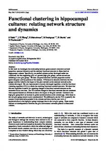
Fig. 1. Comparison of hormone profiles for three women in the Early Pregnancy Study. Frames (a) to (c) show multiple profiles for each woman, while frame the (d) shows the average profile for each woman.

Functional Clustering in Nested Designs

3

with k-means clustering; Heard et al. (2006), where a Bayesian hierarchical clustering approach that relies on spline representations is proposed; Ray & Mallick (2006), who build a hierarchical Bayesian model that employs a Bayesian nonparametric mixture model on the coefficients of the wavelet representations; and Chiou & Li (2007), where a k-centers functional clustering approach is developed that relies on the KarhunenLo`eve representation of the underlying stochastic process generating the curves and accounts for both the means and the modes of variation differentials between clusters. All of the functional clustering methods described above have been designed for situations where a single curve is observed for each subject or experimental condition. Extensions to nested designs where multiple curves are collected per subject typically assume that coefficients describing subject-specific curves arise from a common parametric distribution, and clustering procedures are then applied to the parameters of this underlying distribution. The result is a procedure that generates clusters of subjects based on their average response curve, which is not appropriate in applications in which subjects vary not only in the average but also in the variability of the replicate curves. For example, in studies of trajectories in reproductive hormones that collect data from repeated menstrual cycles, the average trajectory may provide an inadequate summary of a woman’s reproductive functioning. Some women have regular cycles with little variability across cycles in the hormone trajectories, while other women vary substantially across cycles, with a subset of the cycles having very different trajectory shapes. In fact, one indication of impending menopause and a decrease in fecundity is an increase in variability across the cycles. Hence, in forming clusters and characterizing variability among women and cycles in hormone trajectories, it is important to be flexible in characterizing both the mean curve and the distribution about the mean. This situation is not unique to hormone data, and similar issues arise in analyzing repeated medical images as well as other applications. This paper discusses hierarchical Bayes models for clustering nested functional data. We motivate these models using data from the Early Pregnancy Study (EPS) (Wilcox et al., 1998), where progesterone levels were collected for both conceptive and nonconceptive women from multiple menstrual cycles. Our models use splines bases along with mixture priors to create sparse but flexible representations of the hormone profiles, and can be applied directly to other basis systems such as wavelets. We start by introducing a hierarchical random effects model on the spline coefficients which, along with a generalization of the Dirichlet process mixture (DPM) prior (Ferguson, 1973; Sethuraman, 1994; Escobar & West, 1995), allows for mean-responsecurve clustering of women, in the spirit of Ray & Mallick (2006). Then, we extend the model to generate distribution-based clusters using a nested Dirichlet process (NDP) (Rodriguez et al., 2008b). The resulting model simultaneous clusters both curves and subjects, allowing us to identify outlier curves within each group of women, as well as outlying women whose distribution of profiles differs from the rest. To be best of

4

Rodriguez and Dunson

our knowledge, there is no classical alternative for this type of multilevel clustering. In order to provide some insight into the challenges associated with functional clustering in nested designs, consider the hormonal profiles from the EPS depicted in Figure 1. Frames (a) to (c) depict the hormone profiles for 3 women, while frame (d) shows the mean profile corresponding to each one of them, obtained by simply averaging all available observations at a given day within the cycle. When looking at the mean profiles in (d), women 43 and 36 seem to have very similar hormonal responses, which are different from those of woman 3. However, when the individual profiles are considered, it is clear that most of the cycles of woman 43 look like those of woman 3 and that the big difference in the means is driven by the single abnormal cycle. The use of Bayesian nonparametric mixture models for clustering has a long history (Medvedovic & Sivaganesan, 2002; Quintana & Iglesias, 2003; Lau & Green, 2007), and presents a number of practical advantages over other model-based clustering techniques. Nonparametric mixtures induce a probability distribution on the space of partitions of the data, therefore we do not need to specify in advance the number of clusters in the sample. Once updated using the data, this distribution on partitions allows us to measure uncertainty in the clustering structure (including that associated with the estimation of the curves), providing a more complete picture than classical methods. In this paper, we work with a generalized Dirichlet process (GDP) first introduced by Hjort (2000) and study some of its properties as a clustering tool. In particular, we show that the GDP generates a richer prior on data partitions than those induced by popular models such as the Dirichlet process (Ferguson, 1973) or the two parameter Poisson-Dirichlet process (Pitman, 1996), as it allows for an asymptotically bounded number of clusters in addition to logarithmic and power law rates of growth. The paper is organized as follows: Section 2 reviews the basics of nonparametric regression and functional clustering, while Section 3 explores the design of nonparametric mixture models for functional clustering. Building on these brief reviews, Section 4 describes two Bayesian approaches to functional clustering in nested designs, while Section 5 describes Markov chain Monte Carlo algorithms for this problem. An illustration focused on the EPS is presented in Section 6. Finally, Section 7 presents a brief discusson and future research directions.

2.

Model-based functional clustering

To introduce our notation, consider first a simple functional clustering problem where multiple noisy observations are collected from functions f1 , . . . fI . More specifically, for subjects i = 1, . . . , I and within-subject design points t = 1, . . . , Ti , observations

Functional Clustering in Nested Designs

5

consist of ordered pairs (xit , yit ) where it ∼ N(0, σi2 ).

yit = fi (xit ) + it ,

For example, in the EPS, yit corresponds to the level of progesterone in the blood of subject i collected at day xit of the menstrual cycle, and fi denotes a smooth trajectory in progesterone for woman i (initially supposing a single menstrual cycle of data from each woman), and clusters in {fi }Ii=1 could provide insight into the variability in progesterone curves across women, while potentially allowing us to identify abnormal or outlying curves. If all curves are observed at the same covariate levels (i.e., Ti = T and xit = xt for every i), a natural approach to functional clustering is to apply standard clustering methods to the data vectors, yi = (yi1 , . . . , yiT )0 . For example, in the spirit of Ramsay & Silverman (2005), one could apply hierarchical or K-means clustering to the first few principal components (Yeung & Ruzzo, 2001). From a model-based perspective, one could instead suppose that yi is drawn from a mixture of k multivariate Gaussian distributions, with each Gaussian corresponding to a different cluster (Fraley & Raftery, 2002; Yeung et al., 2001). The number of clusters could then be selected using the BIC criteria (Fraley & Raftery, 2002; Li, 2005) or a nonparametric Bayes approach could be used to bypass the need for this selection, while allowing the number of clusters represented in a sample of I individuals to increase stochastically with sample size (Medvedovic & Sivaganesan, 2002). However, in many studies, including the EPS, there are different numbers and spacings of observations on the different subjects. More generally, we can represent the unknown function fi as a linear combination of pre-specified basis functions {bk }pk=1 , i.e., we can write fi (xit ) = θi0 +

p X

θik bk (xit )

k=1

where θ i = (θi0 , θi1 , . . . , θip ) are basis coefficients specific to subject i, with variability in these coefficients controlling variability in the curves {fi }Ii=1 . A common approach to functional clustering is to induce clustering of the curves through clustering of the basis coefficients (Abraham et al., 2003; Heard et al., 2006). Then the methods discussed above for clustering of the data vectors {yi }Ii=1 in the balanced design case can essentially be applied directly to the basis coefficients {θ i }Ii=1 . Although the methods apply directly to other choices, our focus will be on splines, which have been previously used in the context of hormone profiles (Brumback & Rice, 1998; Bigelow & Dunson, 2009); given a set of knots τ1 , . . . , τp , the k-th member of the basis system is defined as bk (x) = (x − τi )q+

6

Rodriguez and Dunson

where (·)+ = max{·, 0}. Given the knot locations, inferences on θ i and σi2 can be carried out using standard linear regression tools, however, selecting the number and location of the nodes τ1 , . . . , τp can be a challenging task. A simple solution is to use a large number of equally spaced knots, together with a penalty term on the coefficients to prevent overfitting. From a Bayesian perspective, this penalty term can be interpreted as a prior on the spline coefficients; for example, the maximum likelihood estimator (MLE) obtained under an L2 penalty on the spline coefficients is equivalent to the maximum a posteriori estimates for a Bayesian model under a normal prior, while the MLE under an L1 penalty is equivalent to the maximum a posterior estimate under independent double-exponential priors on the spline coefficients. Instead of the more traditional Gaussian and double exponential priors, in this paper we focus on zero-inflated priors, in the spirit of Smith & Kohn (1996). Priors of this type enforce sparsity by zeroing out some of the spline coefficients and, by allowing us to select a subset of the knots, provides adaptive smoothing. In their simpler form, zero-inflated priors assume that the coefficients are independent from each other and that θik |γ, σi2 ∼ γN(0, ωk σi2 ) + (1 − γ)δ0 ,

σi2 ∼ IGam(ν1 , ν2 ),

(1)

where δx denotes the degenerate distribution putting all its mass at x, ωk controls the overdispersion of the coefficients with respect to the observations and γ is the prior probability that the coefficient θik is different from zero. In order to incorporate a priori dependence across coefficients, we can reformulate the hierarchical model by introducing 0-1 random variables λi1 , . . . , λip such that yi |θ i , σi2 , Λi ∼ N(B(xi )Λi θ i , σi2 I),

θ i |σi2 ∼ N(0, σi2 Ω),

σi2 ∼ IGam(ν1 , ν2 ),

where yi = (yi1 , . . . , yini ) and xi = (xi1 , . . . , xini ) are, respectively, the vectors of responses and covariates associated with subject i, B(xi ) is the matrix of basis functions also associated with subject i with entries [B(xi )]tk = bk (xit ), and Λi = diag{λi1 , . . . , λip } and λi equals 1 independently with probability γ. Note that if Ω is a diagonal matrix and [Ω]ii = ωi we recover the independent priors in (1). For the single curve case, choices for Ω based on the regression matrix B(xi ) are discussed in DiMatteo et al. (2001), Liang et al. (2005) and Paciorek (2006). Although the preceding two-stage approach is simple to implement using off-theshelf software, it ignores the uncertainty associated with the estimation of the basis coefficients while clustering the curves. In the spirit of Fraley & Raftery (2002), an alternative that deals with this issue is to employ a mixture model of the form yi |{θ ∗k }, {σk∗2 }, {Λ∗k } ∼

K X k=1


wk N B(xj )Λ∗k θ ∗k , σk∗2 I ,

K X k=1

wk = 1,

(2)

Functional Clustering in Nested Designs

θ ∗k

7

Λ∗k

where is the vector of coefficients associated with the k-th cluster, is the diagonal selection matrix for the k-th cluster, σk∗2 is the observational variance associated with observations collected in the k-th cluster, wk can be interpreted as the proportion of curves associated with cluster k, and K is the maximum number of clusters in the sample. From a frequentist perspective, estimation of this model can be performed using expectation-maximization (EM) algorithms, however, such EM algorithm leaves the issue of how many mixture components to use unanswered. Alternatively, Bayesian inference can be performed for this model using Markov chain Monte Carlo (MCMC) algorithms once appropriate priors for the vector w = (w1 , . . . , wK ) and the cluster-specific parameters (θ ∗k , Λ∗k , σk∗2 ) have been chosen, opening the door to simple procedures for the estimation of the number of clusters in the sample. 3.

Bayesian nonparametric mixture models for functional data

Note that the model in (2) can be rewritten as a hierarchical model by introducing latent variables {(θ i , σi2 , Λi )}Ii=1 so that
yi |θ i , σi2 , Λi ∼ N B(xi )Λi θ i , σi2 I

θ i , σi2 , Λi |G ∼ G

G(·) =

K X

wk δ(θ∗k ,σk∗2 ,Λ∗k ) (·).

k=1

(3) Therefore, specifying a joint prior on w and {(θ ∗k , σk∗2 , Λ∗k )}K k=1 is equivalent to specifying a prior on the discrete distribution G generating the latent variables {(θ i , σi2 , Λi )}Ii=1 . In this section we discuss strategies to specify flexible prior distribution on this mixing distribution in the context of functional clustering. In particular we concentrate on nonparametric specifications for G through the class of stick-breaking distributions. A random probability measure G on Rp is said to follow a stick-breaking prior (Ishwaran & James, 2001; Ongaro & Cattaneo, 2004) with baseline measure G0 and L precision parameters {al }L l=1 and {bl }l=1 if G(·) =

K X

wk δϑk (·)

(4)

k=1

where the atoms {ϑk }K k=1 are independent and identically Q distributed samples from K G0 and the weights {wk }K are constructed as w = u k k l=1 s −a yields the two-parameter Poisson-Dirichlet process (Pitman, 1995; Ishwaran & James, 2001), denoted PY(a, b, G0 ), with the choice a = 0 resulting in the Dirichlet Process (Ferguson, 1973; Sethuraman, 1994),

8

Rodriguez and Dunson

denoted DP(b, G0 ). In mixture models such as (3), G0 acts as the common prior for K K the cluster-specific parameters {ϑk }K k=1 , while the sequences {ak }k=1 and {bk }k=1 control the a priori expected number and size of the clusters. The main advantage of nonparametric mixture models such as the Poisson-Dirichlet process as a clustering tool is that they allow for automatic inferences on the number of components in the mixture. Indeed, these models induce a prior probability on all possible partitions of the set of observations, which is updated based on the information contained in the data. However, Poisson-Dirichlet processes have two properties that might be unappealing in our EPS application; firstly, they place a relatively large probability on partitions that include many small clusters, and secondly, they imply that the number of clusters will tend to grow logarithmically (if a = 0) or as a power law (if a > 0) as more observations are included in the data set. However, priors that favor introduction of increasing numbers of clusters without bound as the number of subjects increase have some disadvantages in terms of interpretability and sparsity in characterizing high-dimensional data. For example, in applying DP mixture models for clustering of the progesterone curves in EPS, Bigelow and Dunson (2009) obtained approximately 32 different clusters, with half of these clusters singletons. Many of the clusters appeared similar, and it may be that this large number of clusters was partly an artifact of the DP prior. Dunson (2009) proposed a local partition process prior to reduce dimensionality in characterizing the curves, but this method does not produce easily interpretable functional clusters. Hence, it is appealing to use a more flexible global clustering prior that allows the number of clusters to instead converge to a finite constant. With this motivation, we focus on the generalized Dirichlet process (GDP) introduced by Hjort (2000), denoted GDP(a, b, G0 ). The GDP corresponds to a stickbreaking prior with K = ∞, ak = a and bk = b for all k. When compared against the Poisson-Dirichlet process, the GDP has quite distinct properties. Theorem 1. Let Zn be the number of distinct observations in a sample of size n from a distribution G, where G ∼ GDP(a, b, G0 ) . The expected number of clusters E(Zn ) is given by E(Zn ) =

n X i=1

iaΓ(a + b)Γ(b + i − 1) Γ(b)Γ(a + b + i) − Γ(a + b)Γ(b + i)

The proof can be P seen in appendix A. Note that for a = 1, this expression n b simplifies to E(Zn ) = i=1 b+i−1 ∼ o(log n), a well known result for the Dirichlet process (Antoniak, 1974). Letting Wn = Zn − Zn−1 denote the change in the number of clusters in adding the n-th individual to a sample with n − 1 subjects, Stirling

Functional Clustering in Nested Designs

9

approximation can be used to show that E(Wn ) =

naΓ(a + b)Γ(b + n − 1) ≈ C(a, b)n−a . Γ(b)Γ(a + b + n) − Γ(a + b)Γ(b + n)

where C(a, b) = {aΓ(a + b)/Γ(b)} exp{−2(a + 1)}. Hence, E(Wn ) → 0 as n → ∞ and new clusters become increasingly rare as the sample size increases. Note that for a ≤ 1, the number of clusters will grow slowly but without bound as n increases, with E(Zn ) → ∞. The rate of growth in this case is proportional to n1−a , which is similar to what is obtained by using the Poisson Dirichlet prior (Sudderth & Jordan, 2009). However, when a > 1 the expected number of clusters instead converges to a finite constant, which is a remarkable difference compared with the Dirichlet and Poisson-Dirichlet process. As mentioned above, there may be a number of practical advantages to bounding the number of clusters. In addition, a finite bound on the number clusters seems to be more realistic in many applications, including the original species sampling applications that motivated much of the early development in this area (McCloskey, 1965; Pitman, 1995). In order to gain further insight into the clustering structure induced by the GDP(a, b, G0 ), we present in Figure 2 the relationship between the size of the largest cluster and the mean number of clusters in the partition (left panel), and the mean cluster size and the number of clusters (right panel) for a sample of size n = 1000. Each continuous line correspond to a combination of shape parameters such that a/(a + b) is constant, while the dashed line in the plots corresponds to the combinations available under a Dirichlet process. The plots demonstrate that the additional parameter in the GDP allows us to simultaneously control the number of clusters and the relative size of the clusters, increasing the flexibility of the model as a clustering procedure. The previous discussion focused on the impact of the prior distribution for the mixture weights on the clustering structure. Another important issue in the specification of the model is the selection of the baseline measure G0 . Note that in the functional clustering setting ϑk = (θ ∗k , σk∗2 , Λ∗k ), and therefore a computationally convenient choice that is in line with our previous discussion on basis selection and zero-inflated priors is to write G0 (θ, σ 2 , Λ) = N(θ|0, σ 2 Ω) × IGam(σ 2 |ν1 , ν2 ) ×

p Y

Ber(λs |γ)

(5)

s=1

A prior of this form allows differential adaptive smoothing for each cluster in the data; the level of smoothness is controlled by γ (the prior probability of inclusion for each of the spline coefficients), and therefore it is convenient to assign to it a hyperprior such as γ ∼ Beta(η1 , η2 ).

Rodriguez and Dunson

0.46 0.48 0.5 0.52 0.54

170 160 150

Average size of cluster

640 620

130

● ●

7.0

7.5

8.0

●

8.5

Mean number of clusters

(a)

● ●

●

6.5

0.46 0.48 0.5 0.52 0.54

●

●

600

Size of larger cluster

660

●

140

10

●

●

9.0

●

6.5

7.0

7.5

8.0

8.5

9.0

Mean number of clusters

(b)

Fig. 2. Clustering structure induced by a GDP(a, b, G0 ) for a sample of size n = 1000. Panel (a) shows the relationship between the size of the largest cluster and the mean number of clusters for different GDPs, where each curve shares a common E(uk ) = a/(a + b). Panel (b) shows the relationship between the average cluster size and the mean number of clusters. The dashed lines corresponds to the combinations available under a standard Dirichlet process.

Functional Clustering in Nested Designs

4.

11

Functional clustering in nested designs

Consider now the case where multiple curves are collected for each subject in the study. In this case, the observations consist of ordered pairs (yijt , xijt ) where yijt = fij (xijt ) + ijt , where fij is the jth functional replicate for subject i, with i = 1, . . . , I, j = 1, . . . , ni and t = 1, . . . , Tij . For example, in the EPS, fij is the measurement error-corrected smooth trajectory in the progesterone metabolite PdG over the j-th menstrual cycle from woman i, with t indexing the sample number and xijt denoting the day within the i, j menstrual cycle relative to a marker of ovulation day. A natural extension of (3) to nested designs arises by modeling the expected evolution of progesterone in time for cycle j of woman i as fij = B(xij )θ ij and using a hierarchical model for the set of curve-specific parameters {θ ij } in order to borrow information across subjects and/or replicates. In the following subsections, we introduce two alternative nonparametric hierarchical priors that avoid parametric assumptions on the distribution of the basis coefficients, while inducing hierarchical functional clustering.

4.1. Mean-curve clustering As a first approach, we consider a Gaussian mixture model, which characterizes the basis coefficients for functional replicate j from subject i as conditionally independent draws from a Gaussian distribution with subject-specific mean and variance, in the spirit of Booth et al. (2008): yij |θ ij , σi ∼ N(B(xij )θ ij , σi2 I)

θ ij |θ i , Λi , σi2 ∼ Gi

Gi = N(Λi θ i , σi2 Σ)

(6)

where Λi , θ i , σi2 are as described in expression (3). In this model, the average curve for subject i is obtained as E{fij (x) | Λi , θ i , σi2 } = B(x)Λi θ i , with Λi providing a mechanism for subject-specific basis selection, so that the curves from subject i only depend on the basis functions corresponding to non-zero diagonal elements of Λi . The variability in the replicate curves for the same subject is controlled by σi2 Σ, with the subject-specific multiplier allowing subjects to vary in the degree of variability across the replicates. The need to allow such variability is well justified in the hormone curve application. In order to borrow information across women, we need a hyperprior for the woman specific parameters {(Λi , σi2 , θ i )}Ii=1 . Since we are interested in clustering subjects, a natural approach is to specify this hyperprior nonparametrically through a generalized Dirichlet process centered around the baseline measure in (5), just as we did for the

12

Rodriguez and Dunson

single curve case. This yields (θ i , σi2 , Λi )|G ∼ G

G ∼ GDP(a, b, G0 )

with G0 given in (5). Since the distribution G is almost surely discrete, the model identifies clusters of women with similar average curves. This is clearer if we marginalize out the curve-specific coefficients {θ ij } and the unknown distribution G to obtain the joint likelihood of the data from subject i yi1 , . . . , yini |{wk }, {θ ∗k }, {σk∗2 }, {Λ∗k } ∼ K X k=1

wk

 ni Y 

j=1

 
(7) N B(xij )Λ∗k θ ∗k , σk∗2 (I + Σ) 

By incorporating the distribution of the selection matrices Λ1 , . . . , ΛI in the random distribution G, this model allows for a different smoothing pattern for each cluster of curves. This is an important difference with a straight generalization of the model in Ray & Mallick (2006), who instead treat the selection matrix as a hyperparameter in the baseline measure G0 and therefore induce a common smoothing pattern across all clusters. The model is completed by assigning priors for the hyperparameters. For the random effect variances we take inverse-Wishart priors. Ω ∼ IWis(νΩ , Ω0 )

Σ ∼ IWis(νΣ , Σ0 )

In the spirit of the unit information priors (Paciorek, 2006), the hyper-parameters for these priors can be chosen so that Ω0 and Σ0 are proportional to ni I X X

B(xij )0 B(xij )

i=1 j=1

Finally, the concentration parameters a and b are given gamma priors a ∼ Gam(κa , τa ) and b ∼ Gam(κb , τb ) and the probability of inclusion γ is assigned a beta prior, γ ∼ Beta(η1 , η2 ). 4.2. Distribution-based clustering Because the subject-specific distributions {Gi }Ii=1 were assumed to be Gaussian and the nonparametric prior was placed on their means, the model in the previous section clusters subjects based on their average profile. However, as we discussed in Section 1, clustering based on the mean profiles might be misleading in studies such as the

Functional Clustering in Nested Designs

13

EPS in which there are important differences among subjects in not only the mean curve but also the distribution about the mean. In hormone curve applications, it is useful to identify clusters of trajectories over the menstrual cycle to study variability in the curves and identify outlying cycles that may have reproductive dysfunction. It is also useful to cluster women based not simply on the average curve but on the distribution of curves. With this motivation, we generalize our hierarchical nonparametric specification to construct a model that clusters curves within subjects as well as subjects. To motivate our nonparametric construction, consider first the simpler case in which there are only two types of curves in each cluster of women (say, normal and abnormal), so that it is natural to model the subject-specific distribution as a twocomponent mixture where 2 2 yij |$i , Λ1i , θ 1i , σ1i , Λ2i , θ 2i , σ2i ∼ 2 2 $i N(B(xij )Λ1i θ 1i , σ1i I) + (1 − $i )N(B(xij )Λ2i θ 2i , σ2i I)

(8)

where πi can be interpreted as the proportion of curves from subject i that are in 2 group 1 (say, normal), and (Λ1i , θ 1i , σ1i ) are the parameters that describe curves from 2 a normal cycle and (Λ2i , θ 2i , σ2i ) are the parameters describing the curves from an abnormal cycle. Note that in this case we have not one but two variance parameters for each individual, which provides additional flexibility by allowing each cluster of curves to present a different level of observational noise. This feature is desirable in the EPS because, for a given woman, observational noise in abnormal cycles tends to be larger than in normal cycles. Under this formulation, the subject-specific distribution is described by the vector 2 2 of parameters ($i , Λ1i , θ 1i , σ1i , Λ2i , θ 2i , σ2i ), and clustering subjects could be accomplished by clustering these vectors. We can accomplish this by using another mixture model that mimics (2) and (7), so that ∗2 ∗2 yi1 , . . . , yini |{πk }, {$k }, {θ ∗1k }, {σ1k }, , {Λ∗1k }, {θ ∗2k }, {σ2k }, {Λ∗2k } ∼ K X k=1

πk

ni Y  ∗2 ∗2 $k N(B(xij )Λ∗1k θ ∗1k , σ1k I) + (1 − $k )N(B(xij )Λ∗2l θ ∗2k , σ1k I)

(9)

j=1

As with the simpler model-based functional clustering model we introduced at the end of Section 2, we could generate ML estimators for the parameters of this model using an EM algorithm. However, such an approach still leaves open the question of how many mixture components should be used, both at the subject and curve level. For this reason, we adopt a Bayesian perspective and generalize the model using the nonparametric priors discussed in Section 3. To do so, we start by rewriting (9) as a

14

Rodriguez and Dunson

general mixture model where 2 2 yij |θ ij , σij , Λij ∼ N B(xij )Λij θ ij , σij I




2 θ ij , σij , Λij |Gi ∼ Gi

(10)

and Gi is a discrete distribution which is assigned a nonparametric prior. Note that this is analogous to the formulation in (6), but by replacing the Gaussian distribution with a random distribution with a nonparametric prior we are modeling the withinsubject variability by clustering curves into groups with homogeneous shape. Now, we need to define a prior over the collection {Gi }Ii=1 that induces clustering among the distributions. For example, we could use a discrete distribution whose atoms are in turn random distributions, for example, Gi ∼

∞ X

πk δG∗k

k=1

Q where πk = vk s