Solis, Borkar and Kumar [4] and Giridhar and. Kumar [5] have ... cording to its local clock) just after it receives the packet, de- noted by r. (i,j) ..... San Diego, Dec.
Fundamental Limits on Synchronization of Affine Clocks in Networks∗ Nikolaos M. Freris and P. R. Kumar † Department of Electrical and Computer Engineering, and Coordinated Science Laboratory University of Illinois at Urbana-Champaign Abstract We present some impossibility as well as feasibility results on clock synchronization in wireline or wireless networks. We consider a network of n nodes with affine clocks, where one node is taken as a reference, and each other node’s clock is described by a skew (relative speedup with respect to the reference clock), and an offset (say) at time 0 with respect to the reference clock. In order to establish impossibility results, we allow for noiseless communication of messages that may contain any information that the transmitting node knows about current or past packets that the node has sent or received. The synchronization problem consists of estimating all the unknown parameters, skews and offsets of all the clocks, as well as the delays of all the communication links. We show that, in general, estimation of all unknown parameters is impossible. We show that all nodal skews, as well as all round trip delays between every pair of nodes, can be estimated correctly. However, the unknown link delays and clock offsets can only be determined up to an (n − 1)-dimensional subspace. Each degree of freedom in this subspace corresponds exactly to the offset of one of the n − 1 clocks with respect to the reference node’s clock. On the positive side, we show that every transmitting node can predict precisely the time indicated by the receiver’s clock at the instant it receives the packet. If we further invoke causality, i.e., that packets cannot be received before they are transmitted, the uncertainty set above can be reduced to a compact polyhedron in Rn−1 , which we describe analytically. We also consider a specific model for delays as the sum of a transmitter-dependent delay, a receiver-dependent delay and a propagation delay where the latter is known. We identify conditions on the transmission and reception delays, for which estimation admits a unique solution. ∗ This material is based upon work partially supported by NSF under Con-
tract Nos. CCR-0325716 and CNS 05-19535, DARPA/AFOSR under Contract No. F49620-02-1-0325, DARPA under Contract Nos. N00014-0-1-10576, Oakridge-Battelle under Contract 239 DOE BATT 4000044522 and AFOSR under Contract No. F49620-02-1-0217. † Nikolaos M. Freris and P. R. Kumar, CSL and Dept. of ECE, University of Illinois at Urbana-Champaign, 1308 W. Main Street, Urbana, IL 61801, USA. {nfreris2,prkumar}@uiuc.edu
1. Introduction Distributed clocks generally don’t agree. Yet, several applications in sensor networks and networked control, as well as scheduling in wireless networks, are grounded in accurate time synchronization. This motivates the study of clock synchronization over communication networks. Nodes often need to act in a coordinated fashion in wireless sensor networks or networked control, and accurate knowledge of the exact time is important. Applications include closing control loops in a decentralized system and slotted protocols in communication networks. In sensor networks, time synchronization requirements are omnipresent; in tracking, target localization, data fusion and power-efficient duty-cycling. As we head towards the era of event-cum-time driven systems featuring the convergence of computation and communication with control, the need for well-synchronized clocks becomes vital, affecting both QoS and safety. The specific problem we consider is the characterization of the extent to which synchronization is feasible. We consider clocks which run at constant, but not necessarily identical speed. Thus, each clock is characterized by its “skew,” i.e., relative speed with respect to a reference clock, as well as an “offset,” i.e., the time difference from the reference clock at a particular time, which, for convenience, we take to be the time 0 of the reference clock. Thus, we consider affine clocks. Nodes can exchange packets containing any information. We suppose that packets suffer delays dependent on the transmitter-receiver communication pair; since operating systems, computational loads, CPUs, etc. can vary across platforms. We allow for noiseless communication where latencies in packet transfer are deterministic and time-invariant but unknown. It is important to note that we allow for noiseless communication as well as deterministic delays in timestamping and communication latency since impossibility results proved under such idealistic conditions delineate the fundamental limitations more clearly. We show that all skews can be perfectly determined. However, the delays of links and offsets of nodes cannot be exactly determined. Specifically, the vector of all link delays and node offsets can only be characterized up to a translation of an (n − 1)-dimensional subspace, where n is the number of nodes. In fact, we show that these n − 1 indeterminable
parameters can be regarded as the nodal offset estimates. If we further invoke causality, that packets cannot be received before they are sent, then the uncertainty region can be characterized as a compact polyhedron with non-empty interior. We also address the case where link delays have the structure of being the sum of a transmitter-specific delay, a receiver-specific delay, and a known electromagnetic propagation delay. The rest of the paper is organized as follows. In Section 2 we summarize related literature on clock synchronization. In Section 3, we introduce the affine model for the clocks and the assumptions for the delays. In Section 4, we describe the problem formulation, providing a formal description of the inter-node communication, and generalize an impossibility result for the case of two clocks that was presented in [2]. In Section 5, we prove that with no further assumption on the unknown delays, estimating the offsets is impossible for any network topology and by any communication scheme. We show that while skews can be reliably estimated, offsets involve an inherent indeterminacy. In Section 6, we study the feasibility when the delays have an additive decomposition in terms of transmit, receive and propagation latencies.
2. Related Literature In a distributed system like a wireless network, ordering of events is crucial. Lamport [3] shows how to causally order events by defining the notion of virtual clocks. In applications of networked control and sensor networks, a variety of algorithms have been suggested for synchronization. In most cases, the time difference between clocks is captured by exchanging time-stamped packets, or “pings,” between nodes. The Network Time Protocol (NTP) [7] is a widely used hierarchical protocol implemented to synchronize clocks in large networks like the Internet. NTP provides accuracy in the order of milliseconds ([7], [9]) by typically using GPS to achieve synchronization to external sources that are organized in levels called stratums. While this accuracy is sufficient for most applications, wireless sensor network applications typically require precision in the order of microseconds (µs). Moreover, in some cases, e.g., indoors, or during solar flares, GPS may be unavailable. Sensor network protocols like the Reference Broadcast Synchronization (RBS) and Flooding Time Synchronization Protocol (FTSP) have been developed for this reason. RBS [8] uses transmissions from an intermediate node to synchronize nodes that receive it, by recording and exchanging the receipt times so as to estimate the receiving nodes’ clock differences. It does not make use of time-stamping, but relies on the physical broadcast channel to attain precision within 11 µs. In FTSP [9], the MAC time-stamping capabilities are exploited and linear regression is used to compensate for clock drifts; the precision is in the order of 10 µs. Karp, Elson, Papadimitriou and Shenker [6] study fundamental properties of minimum variance estimates, present algorithms, and analyze the performance in different network topologies. Solis, Borkar and Kumar [4] and Giridhar and
Kumar [5] have designed and implemented a fully decentralized asynchronous algorithm for least-squares estimation of offsets from a reference node, using information about pairwise time differences.
3. Model for Clocks and Delays 3.1. Affine Model for Clocks In general, no two clocks agree. Throughout this paper, we will assume a simple model of affine clocks with constant skew. Denoting the time of a fixed reference clock as t, we will assume that the display of a clock j in the network at time t, denoted by t j (t), satisfies t j (t) := a j t + b j .
(3.1)
We call the ratio of the frequencies of the two clocks a j as the skew, while the difference in their displays will be referred to as the offset at a particular instant. Above, b j is the offset of clock j at time 0. An affine clock can thus be represented by the pair of parameters (a j , b j ), considered constant time-invariant parameters. We suppose that a j > 0, since, in practice, skew takes values very close to 1.1 On the contrary, offsets are sign-indefinite so no constraints are imposed on the values of b j . We will fix the reference node to be node 1; hence a1 := 1, b1 := 0. A useful formula that provides time translation, between two clocks i and j is tj =
aj aj ti + b j − bi . ai ai
(3.2)
3.2. Model for Delay We will suppose that whenever a packet is sent by node i, it is received by node j after a delay of di j time units (measured in the time units of the reference clock). The delays {di j } are assumed to be unknown but fixed. We allow di j 6= d ji and di j 6= dik , since by the word “delay” we mean not only the electromagnetic propagation delay, but also the delay incurred by a packet after it is time-stamped, but before it is transmitted by a node, as well as the delay after it is received but before the time-stamping.
4. Pairwise Synchronization of Two Clocks We begin with the result of Graham and Kumar [2] and further analyze the specifics of pairwise clock synchronization. Let clock 1 (the reference) and clock j be the only two clocks in the system. We consider a sequence of exchanges of time-stamped packets between the reference node 1 and node j. First, we recapitulate the result of [2] that it is impossible to estimate all the unknown parameters, {a j , b j , d1 j , d j1 }. 1 Our analysis essentially requires only that a 6= 0; the only place where j a j > 0 is used is when studying causality.
{a j , a j d1 j , a j d j1 , b j }, of the unknowns in the estimation problem: s1 1 0 1 r1 aj s2 r2 0 −1 1 a j d1 j r3 s3 1 0 1 . (4.8) = s4 r4 0 −1 1 a j d j1 bj .. .. .. .. .. . . . . . Figure 1. Message exchanges between two nodes As shown in Figure 1 (note than in this case i = 1), the two nodes are allowed to communicate repeatedly by exchanging time-stamped packets. In the k-th packet, the transmitting (i, j) node includes its current transmission time, denoted by sk , as measured by its clock just before the transmission. Upon receiving this packet, the receiving node records the time (according to its local clock) just after it receives the packet, de(i, j) noted by rk . When it is unambiguous, as in this section and Figure 1, the superscripts are dropped. For simplicity of notation suppose that odd messages (k odd) correspond to node i transmitting to node j, while even messages (k even) correspond to j transmitting to i. We allow for any packet to contain information about all the past receipt times of all prior packets as recorded at that node, so that each node contains a full log of the transmit/receipt times of packets between them. Equivalently, we can suppose that there is a “genie” that has access to all transmit and receipt times for all packets, as recorded by their respective clocks. Theorem 1 (Impossibility of Pairwise Synchronization, [2]). Even under noiseless communication of an infinite number of packets between the two nodes, estimation of all skew, offset and the two delays is impossible. Proof. Note that by (3.1), if we denote the translation of node j’s time t j to the reference time t by L (t j ), then tj bj L (t j ) := t = − . aj aj
(4.1)
We have (see also Figure 1) k odd: k even:
L (rk ) = sk + d1 j , rk = a j L (rk ) + b j , rk = L (sk ) + d j1 , sk = a j L (sk ) + b j .
(4.2) (4.3) (4.4) (4.5)
Substituting (4.2) into (4.3), and (4.4) into (4.5), we get rk = a j sk + a j d1 j + b j , sk = a j rk − a j d j1 + b j .
Denoting2 the vector on the LHS above by y, the matrix on the RHS by A, and the vector on the RHS by x, we have y = Ax. We observe that y, A contain known information based on the time-stamps, while x is the vector of the unknowns. By the fact that the measurements are noiseless, we know that there exists a solution of y = Ax. A necessary and sufficient condition for this solution to be unique is that the infinite-dimensional matrix A have full-rank, i.e., rank 4. However, in this case, the fourth column of A is the difference between the second and the third column, and so A has rank at most 3. Remark 1.1 The first three columns of matrix A in (4.8) are linearly independent if and only if not all odd (respectively even) entries are the same. Hence the rank of A is considered, w.l.o.g., in the sequel to be exactly 3. Since the above system does not admit a unique solution, it is useful to study the structure of the feasible solution set of the parameters since it represents the uncertainty set. By the fact that the matrix under study has rank 3 while the number of the unknown parameters is 4, and because the noiseless measurements and time invariance of the parameters guarantee consistency, we can restrict our attention to the 4 × 4 principal submatrix of A, which yields the system aj s1 1 0 1 r1 s2 r2 0 −1 1 a j d1 j (4.9) r3 = s3 1 0 1 a j d j1 . r4 0 −1 1 bj s4 Note that (4.9) is equivalent to the full system (4.8), which shows that only four alternating communication pings suffice. For convenience, we denote the finite linear system in (4.9) as y = Ax. The following theorem characterizes precisely what information is deducible and what the structure of the residual uncertainty is. For the remainder of this paper, we use “ ˆ ” as a superscript to denote estimates of unknown quantities, and “ * ” to refer to known quantities derived from the data. Theorem 2 (Characterization of the Uncertainty Set in Pairwise Synchronization). In pairwise synchronization: 1. The skew can be estimated correctly.
(4.6) (4.7)
2. The vector of offsets and delays can only be characterized up to a translated one-dimensional subspace of R3 parametrized by the estimate of the unknown offset. Any
In order to obtain equations that are linear in unknowns, we consider a nonlinear parametrization,
2 By convention, we denote infinite-dimensional vectors and matrices with boldface.
k odd: k even:
point in this translated subspace satisfies (4.8), i.e., is consistent with the data. 3. The round-trip delay can be estimated precisely. 4. If we further use knowledge of causality, that packets cannot be received before they are sent, and also that all skews are strictly positive, then the uncertainty in the offset set reduces to an interval, whose length is proportional to the round-trip delay. Proof. The null space of the matrix A in (4.9) is the subspace of R4 spanned by the vector nA = (0, −1, 1, 1)T . It follows immediately that the skew can be determined without error. Since the null space is one-dimensional, there is exactly one degree of freedom in this solution. We set this one degree of freedom equal to the offset estimate. If we do so and solve for the remaining unknowns, we see that any solution (aˆ j , aˆ j dˆ1 j , aˆ j dˆj1 , bˆ j )T of (4.9) satisfies a∗j aˆ j 0 aˆ j dˆ1 j a∗j d1∗ j = + bˆ j −1 , (4.10) ∗ ∗ 1 aˆ j dˆj1 a d j j1 1 bˆ j 0 where a∗j a∗j d1∗ j a∗j d ∗j1 bˆ j
rk+2 − rk r3 − r1 = = a j, s3 − s1 sk+2 − sk := r1 − a j s1 = r2k+1 − a j s2k+1 , := a j r2 − s2 = a j r2k+2 − s2k+2 ,
:=
∈
R (free parameter).
(4.11) (4.12) (4.13)
(4.15)
where the RHS is deducible from the measured time-stamps. Last, invoking causality, is equivalent to imposing the constraints dˆ1 j ≥ 0, dˆj1 ≥ 0. This and a j > 0 yield bˆ j ∈ [−a∗j d ∗j1 , a∗j d1∗ j ].
(4.16)
By the above characterization of the estimates, an interesting result surfaces: Lemma 3 (Prediction of the Receiving Time by Transmitter). The sending node can determine precisely the time, as measured by the receiver’s clock, at which the receiving node will receive a sent packet. Proof. Manipulation of (4.6), (4.7), and (4.10) yields k odd: k even:
rk = a∗j sk + a∗j d1∗ j , rk =
1 ∗ a∗j sk + d j1 .
where all the quantities on the RHS are deducible.
Theorem 4 (Sufficient conditions for uniqueness of solution). All the parameters {a j , b j , d1 j , d j1 } can be uniquely determined if any one of the following conditions holds: 1. The offset b j , or one of the delays d1 j or d j1 , is known. 2. There is a known affine relationship between the delays in the two directions, i.e., there exist α 6= −1, β known, such that d j1 = αd1 j + β . Proof. The first part follows directly from the fact that both delays are known invertible (since a j 6= 0) affine functions of the offset b j (4.10), and the sum of the delays is known (4.15). For the second part, knowing the sum of the two delays, and an additional linearly independent (since α 6= −1) affine relation between them, yields each of them, and, consequently, the offset. Remark 4.1 Symmetry, d1 j = d j1 , is a special case of Theorem 4.2.
(4.14)
The rest of the results follow from the above characterization. In particular, the parameter a∗j is the unique estimate consistent with the data, and hence the correct estimate of the skew a j . Now, adding the delay estimates dˆ1 j , dˆj1 gives dˆ1 j + dˆj1 = d1∗ j + d ∗j1 ,
When predicting such times, the indeterminacy of offset and delays mutually cancel. This is an important property since predictability of receipt times can be used to measure the accuracy of clock synchronization algorithms. Since the parameter estimation problem does not allow a unique solution for the vector of offset and delays, it is of interest to determine simple additional conditions that will allow precise characterization of offset and delays.
(4.17) (4.18)
5. Network Clock Synchronization Now we turn to the case of networks. We consider a network of n nodes where, again by convention, node 1 is considered to be the reference node. From the results of the previous section, it follows immediately that synchronization is infeasible in the scenario that all nodes are only allowed to bilaterally exchange packets with the reference node, regardless of the actual number of the packets to be exchanged. This is equivalent to having independent parallel pairwise synchronizations of all the nodes, i.e., a star synchronization graph. Note also that in the case of a star graph, there are exactly n − 1 degrees of freedom in the uncertainty set, corresponding to the estimates of the unknown offsets of the n − 1 clocks with respect to the reference clock. The delay estimates are characterized as affine functions of these offset estimates. However, in the multi-node case, it is not trivial to see what is or is not determinable when the nodes are allowed to collaborate. Hence, it is interesting to analyze the case where all nodes are allowed to exchange packets bilaterally, i.e., to study the case of a complete synchronization graph. We will show that even such full collaboration leads to exactly the same uncertainty set as the star graph, thus proving that the indeterminacy set is the same for intermediate sets of collaborations, as well. In fact, Theorem 6 proves that this is so when the set of links, for which the pair of nodes at the ends
of each link exchange packets, constitutes a connected graph and includes every node in the network. The parameter estimation problem in this setting becomes nonlinear, when communication between nodes other than the reference node is enabled. This can be seen from the nonlinear dependency of (3.2) on the unknown parameters {a j , di j }. Nonetheless, the results of the above section carry over to this case through the following corollary. Corollary 5 (Pairwise Synchronization between two nodes other than the reference node). In pairwise synchronization between two nodes i, j neither of which is the reference node, the same impossibility results and structure of the solution presented in the previous section hold, with the relative skew aj ai taking the place of the skew a j , and the relative offset b j − aj ai bi in place of the offset b j . Proof. Using equation (3.2) for time translation between nodes i and j, Figure 1, and the same line of reasoning as in Theorem 1, we get
(i, j)
r1 (i, j) s2 (i, j) r3 (i, j) s4 .. .
=
(i, j)
s1 (i, j) r2 (i, j) s3 (i, j) r4 .. .
1 0 0 −1 1 0 0 −1 .. .. . .
1 1 1 1 .. .
aj ai a j di j a j d ji b j − a j bi ai
.
(iv) If causality is also exploited, the feasible set for the estimates {bˆ i : 2 ≤ i ≤ n} of the offset parameters {bi : 2 ≤ i ≤ n} can be fully characterized as a compact polyhedron of Rn−1 with a non-empty interior. Remark An important consequence is that the star graph is still feasibility-optimal in the sense that it results in the exact same uncertainty set for the parameters, if causality is not invoked. If causality is additionally taken into account, then the collaborations do help to reduce the size of the uncertainty set. Sketch of proof. The complete proof can be found in [1]. Here we highlight the key points in five steps: 1. Multiplying the relative skews along a spanning tree rooted at the reference node allows us to estimate all nodal skews; this establishes (ii). 2. Introduce the following nonlinear over-parametrization: a
a
• { aij , a j di j , a j d ji , b j − aij bi } for i = 2, 3, . . . , n, and j = i + 1, i + 2, . . . , n,
(5.1) Therefore the previous results continue to hold for this new parametrization. We consider a 4 × 4 system of rank 3, derived from (5.1) by considering four distinct communication pings. For compactness of representation we denote this system by y(i, j) = A(i, j) x(i, j) .
(iii) All the unknown delays {di j } can be expressed as known affine combinations of only n − 1 variables {bˆ i : 2 ≤ i ≤ n}, which can be regarded as estimates of the unknown offsets bi . Any choice of these estimates is consistent with the data of all transmit and receipt times of all packets.
(5.2)
Observe that the unknowns are ai , bi , i = 2, 3, . . . , n and di j , i, j = 1, 2, . . . , n, i 6= j, for a total of 2(n − 1) + n(n − 1) = (n + 2)(n − 1) unknown parameters. The following theorem establishes the fundamental result that without any further assumptions, clock synchronization is impossible in a network of n collaborating clocks. It also demonstrates that the feasible solution set is a fully characterized polyhedron. Theorem 6 (Infeasibility of Clock Synchronization in Networks and Polyhedral Structure of Feasible Set). Consider a network of n nodes where from every node i there is a path to node 1 consisting of links such that every pair of nodes connected by a link, bilaterally exchange packets. (i) It is impossible to estimate all (n + 2)(n − 1) unknown parameters ai , bi , i = 2, 3, . . . , n, and di j , i, j = 1, 2, . . . , n, i 6= j, even under noiseless, infinitely many communication pings between all pairs of nodes. (ii) However, all the skews {ai : 2 ≤ i ≤ n} can be estimated correctly.
• {a j , a j d1 j , a j d j1 , b j } for j = 2, 3, . . . , n. This involves four unknowns per communication link, for a total of 2n(n − 1) in the case of a complete graph. This introduces an additional (n − 1)(n − 2) redundant parameters. 3. The new system is linear and fully decoupled in the communicating pairs. For each bilateral communication link, every solution to the estimation of the relative skew and the link delays is of the form
aj (d ai ) \ (a j di j ) \ (a j d ji ) a \ (b − j b ) j
a ( aij )∗ (a j di j )∗ = (a j d ji )∗ 0
0 + θˆi j −1 , (5.3) 1 1
ai i
where the one degree of freedom, denoted by θˆi j , corresponds a to the estimate of the relative offset b j − aij bi . If we denote this system by xˆ(i, j) = x∗ (i, j) + θˆi j nA , then the solution for the entire network takes the following matrix form xˆ(1,2) . . (i,. j) xˆ . . . (n−1,n) xˆ
∗ (1,2) x . . . = x∗ (i, j) . . . ∗ (n−1,n) x
nA . . . + θˆ12 0 . . . 0
0 . . . + · · · + θˆi j nA . . . 0
+ · · · + θˆn−1,n
0 . . . 0 , . . . nA (5.4)
where 0 := (0, 0, 0, 0)T . 4. We exploit the redundancy in the parametrization. Since all skews are deducible, for offset consistency we need that
a aˆ a θˆi j := (b j\ − aij bi ) = bˆ j − aˆij bˆ i = bˆ j − aij bˆ i , i.e., we obtain a known linear expression of θˆi j with respect to the nodal offset estimates {bˆ j }nj=2 . All unknown delays and relative offsets are affine functions of the nodal offsets. This proves (i) and (iii). 5. Causality is equivalent to di j ≥ 0. Using also ai > 0, we obtain aj (5.5) −a j d ∗ji ≤ bˆ j − bˆ i ≤ a j di∗j , ai which combined with (4.16) yields the feasible set as a compact polyhedron which has a non-empty interior iff all roundtrip delays are strictly positive.
6. Analysis of a Structured Model for Delays We now address the case where the delay has additional structure. Let us suppose (see also [10] and [9]) that the delay in the directed communication pair (i, j), di j , consists of the sum of three terms: 1 . A transmission delay αi which accounts for the processing time in the transmitter after time-stamping. This is assumed to be fixed and transmitter-dependent. 2. An electromagnetic propagation delay τi j which can be estimated correctly, say by GPS, or other position information. 3. A receiving delay β j which accounts for the processing time in the receiver before time-stamping. This is also assumed to be fixed and receiver-dependent. To sum up, the model for delay is di j = αi + τi j + β j , i, j = 1, 2, . . . , n and i 6= j.
(6.1)
However it can be seen that adding ε > 0 small enough to all αi ’s and simultaneously subtracting the same value ε from all βi ’s, will make no difference. Hence, in general, this structured delay model is still unsolvable. We can also consider the case where there is an unknown affine relation between the transmission and receiving delays, i.e., αi = γβi + δ for all nodes, where the parameters γ, δ are unknown and γ ≥ 0. For each fixed pair (γ, δ ), we obtain a known affine characterization of the asymmetry, hence there exists a unique solution, by Theorem 4. As one ranges over various γ > 0, and δ , one obtains an uncertainty set parametrized by two degrees of freedom, namely γ, δ . An interesting special case is when δ = 0. This corresponds to the case where nodes run at a constant but unknown speed, and transmission and receiving delays are simply inversely proportional to the speed of the processor at the node. In this case, the uncertainty set is parametrized by a single degree of freedom, γ > 0. A more general analysis of affine structured models for delays can be found in [1].
7. Concluding Remarks We have characterized what is fundamentally feasible and infeasible in synchronizing affine clocks over a wired or wireless network. The main result is that the estimation of the
unknown parameters offsets and delays is, in general, impossible, though the skews can be estimated correctly. This result has been established under the most favorable scenario of noiseless time-stamping, and therefore, continues to hold when noisy measurements are made. We have also characterized the uncertainty set. The delays can be estimated up to the unknown nodal offsets, with the latter being indeterminable parameters. Moreover, invoking causality, we have shown that the offset vector lies in a completely characterized compact polyhedron with non-empty interior. If there is a known asymmetry in the delays that can be affinely characterized, a unique solution exists. Last, we have studied the special case where the delay has structure as the sum of transmission and receiving delay plus a known electromagnetic propagation time, and provided sufficient conditions for uniqueness of solution.
References [1] Nikolaos M. Freris, Scott R. Graham, and P. R. Kumar, ”Fundamental Limits on Synchronizing Clocks over Networks.” Submitted to IEEE Transactions on Automatic Control 2007 - Under review. [2] Scott Graham and P. R. Kumar, “Time in general-purpose control systems: The Control Time Protocol and an experimental evaluation.” Proceedings of the 43rd IEEE Conference on Decision and Control, pp. 4004-4009. Bahamas, Dec. 14-17, 2004. [3] L. Lamport, “Time, Clocks and the Ordering of Events in a Distributed System.” Communications of the ACM, vol. 21, no. 7, pp. 558-565, July 1978. [4] R. Solis, V. Borkar and P. R. Kumar, “A New Distributed Time Synchronization Protocol for Multihop Wireless Networks.” Proceedings of the 45th IEEE Conference on Decision and Control, pp. 2734-2739, San Diego, Dec. 13-15, 2006. [5] Arvind Giridhar and P. R. Kumar, “Distributed Clock Synchronization over Wireless Networks: Algorithms and Analysis.” Proceedings of the 45th IEEE Conference on Decision and Control, pp. 4915-4920, San Diego, Dec. 13-15, 2006. [6] J. Elson, R.M. Karp, C.H. Papadimitriou and S. Shenker, “Global Synchronization in Sensornets.” Proceedings of LATIN, 609-624. [7] D. L. Mills, “Internet Time Synchronization: The Network Time Protocol.” IEEE Trans. Communications, vol. 39 no. 10 pp. 1482-1493, Oct 1991. [8] J. Elson, L. Girod and D. Estrin, “Fine-Grained Network Time Synchronization using Reference Broadcasts.” Proceedings of the Fifth Symposium on Operating Systems Design and Implementation (OSDI 2002), Boston, MA, December 2002. [9] M. Maroti, G. Simon, B. Kusy, and A. Ledeczi, “The Flooding Time Synchronization Protocol.” Proceedings of the Second International Conference on Embedded Networked Sensor Systems, Baltimore, MD, USA, Nov. 2004, pp. 39-49. [10] H. Kopetz and W. Ochsenreiter, “Clock Synchronization in Distributed Real-Time Systems.” IEEE Transactions on Computers, C-36(8), p. 933-939, August 1987.