Fundamental limits to quantum computation: the energy cost of precise quantum logic J. Gea-Banacloche Department of Physics, University of Arkansas, Fayetteville, AR 72701∗ (Dated: November 28, 2005) Quantum computation requires the precise manipulation of very large coherent superpositions of quantum-mechanical states. Fundamental principles of quantum mechanics (broadly speaking, the uncertainty principle) set constraints on the size of the apparatus needed to perform such manipulations. In many cases, this would translate into a minimum energy requirement for accurate quantum logic.
I.
separate systems; that is, the new basis states are objects that can symbolically be written as
QUANTUM COMPUTING: AN INTRODUCTION
The first motivation for thinking about quantum computers may go back to Feynman [1], who, in 1982, remarked on the intrinsic difficulties of simulating the physics of quantum systems on classical computers, and suggested that what one would need for this purpose would be quantum computers. The difficulty with classical computers that Feynman pointed out can be simply explained as follows. An arbitrary state of a quantum-mechanical system is, in general, a vector in a Hilbert space of dimension N . For a particle in ordinary, three-dimensional space, a familiar representation of its state makes use of a wavefunction, which is mathematically a vector in an infinite-dimensional space such as L2 (the space of square-integrable functions); nonetheless, for practical (ccomputational) purposes, one uses most often a discretized and truncated representation of the wavefunction. For instance, one can introduce a spatial grid, and a vector that contains the values of the wavefunction sampled at the grid points; or one could expand the wavefunction on a complete, discrete (and, in general, infinite) set of orthogonal functions, and work with the vectors containing the coefficients of this expansion, truncated after a suitable order in the expansion. Either way, the result is, for practical purposes, a vector in a Hilbert space of finite (but usually large) dimension N . If the basis states are symbolically represented as |ni, with n = 0, . . . , N − 1, then the general state of the system can be written as |ψi =
N −1 X n=0
Cn |ni
(1)
with some coefficients Cn . Now consider what happens when a second, identical system is added, and allowed to interact with the first one. It is a fundamental postulate of quantum mechanics that the description of the joint system requires a vector space that is a tensor product of the spaces of the two
∗
[email protected]
|n1 i ⊗ |n2 i
(2)
with both indices n1 and n2 running from 0 to N − 1. Therefore, the resulting Hilbert space has dimension N 2 , which is typically a number much larger than N . In fact, it is clear that as more particles are added to the problem, the dimension d of the total Hilbert space increases exponentially with the number of particles n: d = N n . This means that N n coefficients are needed to describe the most general state of the system of n particles—an impossibly large number, as soon as n becomes moderately large, even for very small N . Very soon, one finds it impossible to even store all the coefficients in memory (not to mention manipulate them) in a conventional, classical computer. This is a difficulty that is constantly faced by scientists working on, for instance, quantum chemistry (attempting to describe atoms and molecules form first principles using quantum mechanics), or theoretical solid state physics. In this context, Feynman’s idea is very simple and very sensible. To deal with the exponential growth of the Hilbert space, use as the “computer” a physical system with a comparably large “working space”—which is to say, another quantum system. The result, which might be called a quantum simulator, is conceptually closer to conventional analog computers than to general-purpose digital classical computers. Basically, it would consist of a system, S, of quantum “objects” over which one has very precise experimental control, and whose evolution can be followed with great accuracy. By establishing a precise mathematical correspondence between observables in S and observables in the system O that is the true object of the study, and between their respective dynamics, one could in principle learn anything about a property of O (including, for instance, how it evolves in time, or how it varies with some external parameters) by measuring the corresponding property in S. This general idea of a quantum simulator remains, in this author’s opinion, one of the most attractive potential applications of quantum computers, and probably the one that will be most easy to implement in the not-too-distant future. In the years following Feynman’s proposal, a number of scientists started to look into the possibilities of digital quantum computation; they introduced formal models of
2 digital computers, based on the laws of quantum mechanics (in particular, the principle of superposition, as embodied in the linear structure of the Hilbert space and of the Schr¨odinger equation), and asked whether these devices could do some things that classical Turing machines (the archetype of universal classical computers) were incapable of. The basic physical element of a digital quantum computer is the quantum bit or qubit. A qubit can be any quantum system whose Hilbert space is (for practical purposes) two dimensional. Its basis states can therefore be written as |0i and |1i, and these are, in fact, identified with the corresponding “0” and “1” states of a classical bit. But, in addition, the quantum system can also be in any of an infinite set of other possible states, given by |ψi = C0 |0i + C1 |1i
(3)
with all the possible values of C0 and C1 compatible with the normalization condition |C0 |2 + |C1 |2 = 1. The state (3) is called a “coherent superposition” state, and, for general values of C0 and C1 it corresponds to the qubit being in some sense in both the |0i and |1i states simultaneously, in much the same way as, in the classical double-slit interference experiment with single photons, each photon passes through both slits simultaneously (much more on this in the next section). This principle of superposition is at the root of the “quantum parallelism” characteristic of quantum computers. To see how it works, consider a set of two qubits. Classically, a two-bit register can be used to store (in binary) any of the numbers 0, 1, 2 or 3. Quantummechanically, any of these numbers corresponds to a basis state of the two-qubit Hilbert space. For instance, the number 2 ≡ 10 in binary would be stored as the two-qubit state |2i ≡ |1i ⊗ |0i = |1i|0i = |10i
(4)
(The above line gives an idea of the various equivalent notations that can be used for the same state.) Now, consider what happens if, starting from the state |00i, we apply a Hadamard transform to both qubits. This is a unitary operation that √ turns the state |0i into the superposition (|0i + |1i)/ 2 and the state |1i into (|0i − √ |1i)/ 2. The final state of the register is then 1 1 1 √ (|0i+|1i)⊗ √ (|0i+|1i) = (|00i+|01i+|10i+|11i) 2 2 2 (5) and we can see that now “somehow” all the possible values from 0 to 3 are “in” the register, in superposition form. Clearly, the idea generalizes: if we have a register of n qubits, n Hadamard transforms suffice to “initialize it” into a coherent superposition of all the 2n values that could be stored in a classical register of that size—all of them, in some sense, present simultaneously. Now suppose that we have a physical way to apply a transformation to the register that corresponds to some
mathematical operation—a multiplication, or division, or something like that. By the linearity of quantum mechanics, the operation will act on all of the possible values of the input simultaneously, yielding a degree of parallelism that is exponential in the number of qubits. Ultimately, of course, we do not want (nor would we be able to extract) all of the values of the coefficients in the large superposition state that would result from these operations; what we hope is that some combination of these will produce a useful result, essentially a set of at most n bits that will correspond to the answer to some interesting mathematical problem. The first indication that one could use these ideas— superposition and quantum parallelism—to answer a query in fewer computational steps than with a classical computer was provided by the Deutsch algorithm in 1985 [2] (see [3] for a detailed discussion). The real breakthrough, however, did not come until 1994, when Peter Shor [4] announced an algorithm for, in essence, obtaining the order of an integer a modulo another integer b (a < b) in a number of steps of the order of L3 , where L = log2 b. The order r is the lowest strictly positive integer such that ar mod b = 1 (assuming a and b have no common factors). This is believed to be a “hard” problem for classical computers, which means that no classical algorithms are known that can calculate r in a number of steps that is a polynomial in L. Shor’s method requires, naturally, enough qubits to store the input numbers a and b, and, later, the answer, r, which is always ≤ b. The problem seems ideally suited for quantum computers, because it can be specified with relatively few bits of information (of the order of L) and the output involves also relatively few bits, but the “na¨ıve” way to approach it, on a classical computer, would require generating a large (exponential in L) number of intermediate results that in themselves are not really interesting at all. These would be the values of a1 mod b, a2 mod b, a3 mod b, . . ., and so on, until one finally hits the correct exponent r. The quantum algorithm somehow simultaneously “calculates” all these numbers by preparing a register x in a superposition of all the values of x from 0 to b − 1, and then evaluating in parallel ax mod b for all these values; then it does something to the coefficients of the resulting superposition state that ensures that a number from which one could determine r gets written to an appropriate register. In some sense, therefore, in the intermediate stages, the quantum computer does use the exponentially large amount of potential information represented by all the values of ax mod b, but it only uses this to generate, in the end, an amount of information, in bits, strictly smaller than the input. To be slightly more precise, note that the function f (x) = ax mod b is periodic with period r (since f (0) = f (r) = 1), and all we want is to determine this period. The quantum computer accomplishes this task by using what is called the “quantum Fourier transform” algorithm, which acts on a superposition state to convert it into another superposition whose coefficients are
3 given by the (discrete) Fourier transform of the original coefficients. This gives us just what we need, because the Fourier transform of a periodic function consists of “peaks” at the fundamental frequency and its multiples. A measurement of the appropriate register at the end of the calculation will then yield a state whose amplitude in the superposition is large, i.e., it corresponds to one of the peaks in the Fourier transform, and therefore the number corresponding to that basis state must be a good approximation to an integer multiple of 1/r; a few runs of the algorithm are then sufficient to determine r from this information, with high probability (see [3] or [5] for the full details). Shor’s algorithm is important for several reasons, of which the main one is that the problem of factoring a large integer b can be reduced to the problem of finding the order of a mod b, where a is an (almost) random number in the range 0 < a < b. Factoring, in turn, is an important problem in cryptographic applications: the security of RSA (a form of public-key encryption) cryptography depends on the computational difficulty of factoring, with today’s computers, numbers of more than 500 bits. A quantum computer would thus be able to break today’s most-widely used public-key encryption codes in virtually no time at all. Shor’s discovery, therefore, made quantum computers extremely interesting to the Intelligence agencies, and this is what primarily accounted for the large sums of money that have been invested, and continue to be invested, on quantum computing research since then.
II.
COHERENCE AND DECOHERENCE
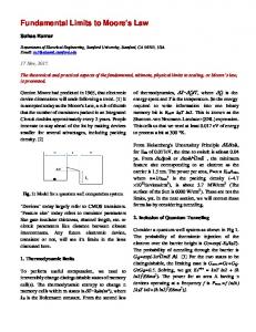
It was very soon realized that the main challenge to the realization of a large-scale quantum computer would come from the phenomenon generally known as “decoherence.” “Coherence” is a word used mostly in optics, where it refers to the ability of light from different sources to produce observable interference patterns. For instance, in the classic double-slit experiment, one can only see an interference pattern if the light coming from both slits is (mutually) coherent (figure 1a); more precisely, the visibility of the interference pattern is a measure of the degree of mutual coherence between the light at both slits. When the slits are illuminated by spatially incoherent light, no interference is seen (figure 1b). This traditional optical concept of coherence is closely related to its quantum mechanical counterpart. In fact, in the quantum-mechanical description of the double-slit experiment, each photon “goes through both slits simultaneously” and as a result interference fringes are formed that contain information about, for instance, the spacing between the slits—something that would not be possible if each photon went through only one slit. In this situation, if |0i represents, symbolically, the state in which a photon goes through slit “0”, and |1i the state in which it goes through slit “1”, the physical state could be written
(a)
(b) FIG. 1: (a) Interference fringes in a double-slit arrangement produced when each photon goes through both slits simultaneously. This is a coherent superposition of the two situations depicted in (b), where each photon goes through only one slit. An incoherent superposition of the two patterns shown in (b) would exhibit no interference fringes.
as the superposition 1 |ψi = √ (|0i + |1i) 2
(6)
and we call this superposition “coherent” precisely because the physical system displays interference. On the other hand, an incoherent superposition (or mixture) of the two alternatives, described by the density matrix ρinc =
1 1 |0ih0| + |1ih1| 2 2
(7)
does not display interference, and corresponds to the situation where each photon goes through one slit or the other, not both at once; that is, it corresponds to the completely incoherent case of classical optics. Note that the state |ψi of Eq. (6) also admits of a density matrix representation, which would be ρcoh = |ψihψ| =
1 1 1 1 |0ih0|+ |1ih1|+ |0ih1|+ |1ih0| (8) 2 2 2 2
Comparing Eq. (7) with (8), we see that the difference between the coherent and incoherent case lies in the absence of off-diagonal elements in (7). In general, the degree of “decoherence” of a superposition state can be measured from the relative size of these off-diagonal elements, in some appropriate basis. The reason why decoherence is an important problem for quantum algorithms can be illustrated by considering again Shor’s order-finding algorithm. At some point, this requires performing the quantum Fourier transform on a register of about L qubits that may be in a state such as |a0 i + |a0 + ri + |a0 + 2ri + . . . + |a0 + nri
(9)
4
FIG. 2: Coherent light diffracted by an array of many slits (a grating) exhibits very sharp interference maxima whose spacing reflects the spacing of the slits in the diffracting screen (the period of the grating). Observing the location of a few of these maxima may be enough to infer the period of the grating, and this could be accomplished, in principle, with just a few photons. Shor’s period-finding algorithm in a quantum computer works in a very similar way, but the coherent superposition is prepared in a mathematical Hilbert space, rather than in “real” space.
where n may be a large number, perhaps of the order of 2L−1 . Now, recall that in classical optics the electromagnetic field diffracted by a plane screen is, far from the screen, given by the Fourier transform of the field on the screen plane. Hence, the quantum computer’s task is, formally, completely equivalent to obtaining the distribution, in the far field, of light that has been put through a set of equally-spaced slits (with r acting as the spacing); see Fig. 2. Then, just as the optical system will not produce a proper Fourier transform (from which one could infer the value of r) unless the light coming from all the slits is coherent, the quantum Fourier transform will fail if the superposition (9) is not fully coherent: the quantum Fourier transform relies on quantum interference in just the same way as the optical Fourier transform relies on optical interference. But how does a quantum-mechanical superposition lose coherence? Again the double-slit example provides an answer. We are familiar with the statement that it is impossible to simultaneously observe interference and determine through which slit the photon went. Physically, this means that any attempt to locate the photon at either one of the two slits destroys the interference pattern, and hence the underlying state coherence. The general principle may be stated thus: if the photon leaves any indication behind of having passed through one slit, and not the other, the coherence of the state is lost, at least in part—it is lost completely if the record leaves no doubt as to which slit the photon went through. Remember the interpretation of a superposition such as (9) as representing a situation in which the system is in some sense “simultaneously” in all of the states shown. Then what we are saying is that coherence will be lost if the “environment” (anything with which the system of qubits might interact in its surroundings) has any way to tell the states apart, to measure, however imperfectly, the system as being in one of them and not the others.
Suppose, for instance, that the qubits were spins, and the states |0i and |1i represented “spin up” and “spin down”, respectively. Then the states being superimposed in (9) would all correspond to different local magnetic fields (since every spin carries with it a magnetic field). Anything in the environment that could tell the difference between, for instance, a state with two spins up, |00i, and a state with two spins down, |11i could, at least in part, destroy the coherence of a superposition √ like (|00i + |11i)/ 2, by responding to the magnetic field of the qubits in a way that would identify one of the two possibilities, and not the other one, as being actually present at that location.
Now, a coherent superposition like (9) would, in a typical application of Shor’s algorithm, contain an extremely large number of states, exponential in L—after all, as discussed in the introduction, it is precisely this exponentially large Hilbert space that gives the quantum algorithm its advantage over the classical one. To preserve the coherence requires to arrange for the interaction with the environment to be so weak that none of these terms leaves a distinctive trace on the environment, at least, for as long as the computation lasts. This is a daunting task: it has long been known that, under fairly general circumstances, the rate at which a superposition decoheres tends to be, itself, exponential in the physical size of the system, so that a superposition state of L qubits would decohere approximately 2L times faster than a superposition state of just one qubit. If this scaling applies generically to quantum computers, it would precisely negate their calculational advantage, since the time available for the computation would shrink exponentially.
The above point was soon made by a number of scientists, such as Unruh [6] and, perhaps most famously, Haroche and Raymond [7], in a special column in Physics Today. Ironically, even at the same time as these observations were being published, a solution was being worked out. This was the realization that quantum error correction was possible, and moreover, that it was possible to do it fault-tolerantly [8]. The practical meaning of this, probably the most important discovery in the history of quantum information processing, was that, as long as one could perform error correction on a system of qubits before it had had a chance to decohere much, the initial coherent superposition could be restored with high probability, and the process could be kept up, for as long as necessary, provided that the error probability per qubit (due to all error sources, including decoherence) per error correction step was kept below a certain threshold value. Estimates of the threshold vary, depending on assumptions about the computer’s architecture and the error-correction process itself, but it is probably safe to set it around 10−4 for most practical purposes.
5 III. ERRORS DUE TO THE QUANTUM NATURE OF THE CONTROL SYSTEMS
From the point of view of error correction, anything that may cause a qubit to be in a state other than the one it was supposed to be in is an error. The error probability can be quantified, if the actual density operator ρ for the system is known, by comparing it to whatever it was supposed to be, say, ρ0 . The overlap of these operators, as measured, for instance, by the trace of their product, gives the probability that no error occurred, and 1 − T r(ρρ0 ) gives the error probability: Pe = 1 − T r(ρρ0 )
(10)
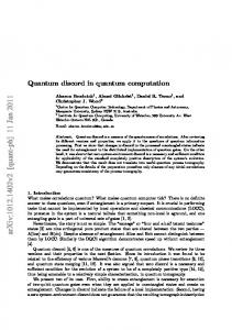
(it is easy to see, for instance, that if a qubit has decohered to the point that its state is given by (7) instead of (8), equation (10) predicts an error probability of 1/2). Decoherence of the qubits due to their interaction with the environment is just one of several possible sources of errors. Others include imperfections in the control systems that need to act on the qubits in order to perform the logical operations needed for the computation (such as, e.g., the Hadamard transforms introduced in Section 1). For instance, a particular radiation pulse could be too strong or too long, or have the wrong relative phase. A few years ago a number of authors, simultaneously and independently, started to explore the errors that would be introduced in quantum computation by the quantum nature of these control systems (in what follows we will most often refer to these as control fields, since they would typically be electromagnetic fields applied to the qubit system). It is interesting to observe that there is also a clear parallel here with the discussions of the double-slit interference experiment, mostly by Einstein and Bohr [9], at the dawn of quantum mechanics. When Einstein suggested that a movable screen could in principle be used to obtain information on which slit the photon went through, Bohr countered that the screen itself would then, for consistence, have to be described by quantum mechanics, in which case the uncertainty principle applied to the screen would prevent the simultaneous determination of the path taken by the photon and the observation of the interference pattern. Einstein’s idea (or, rather, a popular, somewhat modified version of it, perhaps due to Feynman [10]) is schematically illustrated in Figure 3. For a photon that reaches a particular point on the screen, a movable screen would experience a different momentum recoil depending on whether the photon passed through the upper or the lower slit. If this momentum could be measured, one could tell which way the photon went. There are a number of ways to see why this would not work, if the screen is treated as a quantum, rather than a classical, object . Perhaps the most fundamental one is to note that the full state of the system would then be, instead of (6), the joint (entangled) state of photon and
p0 d p1
D FIG. 3: Einstein’s concept of a double-slit screen, on frictionless rollers, that can move in the transverse direction. Each of the two possibilities shown for a difracted photon (p0 and p1 ) leaves the screen in a different transverse momentum state. By measuring this momentum, one could determine, in principle, which way the photon went. However, Bohr showed that, in this case, the quantum-mechanical nature of the screen would cause the interference fringes to disappear.
screen 1 |ψi = √ (|0i|p0 i + |1i|p1 i) 2
(11)
where |p0 i and |p1 i represent the states of the screen after it has given the photon a transverse momentum p0 or p1 , respectively. When one traces over the state of the screen, one finds the following reduced density operator for the state of the photon 1 1 ρ = |0ih0| + |1ih1| 2 2 1 1 + hp1 |p0 i|0ih1| + hp0 |p1 i|1ih0| 2 2
(12)
This is a partly decohered state, which becomes a completely incoherent state (like (7)) if the states |p0 i and |p1 i are orthogonal, in which case they are perfectly distinguishable. In this case, the interference completely vanishes, as discussed in connection with (7) and illustrated in Figure 1b. An alternative approach invokes the uncertainty principle as applied to the screen. To be able to determine the photon’s path, the uncertainty in the screen’s transverse momentum must be ∆p < |p0 − p1 | ≃ ¯hd/λD. But then its position uncertainty is ∆x ≥ ¯h/∆p = λD/d, which is just of the order of magnitude of the width of the interference fringes. With such a large uncertainty in the position of the screen, the patterns formed by successive photons would not overlap properly, and no interference would be visible. Either way, we may conclude that, when a quantum system, like the photon in this example, interacts with a seemingly classical apparatus, treating the apparatus quantum-mechanically generally results in decoherence,
6 i.e., a loss of the system’s quantum ability to interfere. We may expect the same thing to happen when the quantum nature of the control systems used for quantum computation is taken into account. Indeed, this was shown to be the case in some of the first papers to address this question, which roughly followed, independently, the same two approaches sketched above. Thus, Van Enk and Kimble [11] considered the entanglement between an atomic qubit and a quantized laser field, whereas Gea-Banacloche [12] considered the errors in the state evolution that would arise from the fluctuations in the phase and intensity of the quantized field (for a quantum field, phase and intensity are approximately conjugate variables, similarly to position and momentum for a material particle). At about the same time, Ozawa [13] had been exploring the similarity between certain quantum logical operations and measurements, and focused on the constraints imposed on quantum measurements by conservation laws, originally discussed by Wigner, Araki and Yanase (WAY) [14, 15]. Note that a conservation law (namely, conservation of momentum) is the basis of the proposed used of the screen as a measuring device in the double-slit experiment, as well as the reason for the entanglement exhibited by the state (11). There are a number of ways in which different quantum logic operations can be reinterpreted as stages in a measurement of some qubit operator, and restrictions on the operation can then be derived from the WAY theorem, which states that any observable that does not commute with an additively conserved quantity cannot be measured with absolute precision. In a series of papers, Ozawa [13, 16] was able to express these constraints as requirements on the “size” of the auxiliary (or control) system needed in order to be able to perform the operation approximately, to some desired accuracy. For bosonic controls, such as electromagnetic fields, these constraints amount to the observation that the minimum error probability scales as 1/¯ n, where n ¯ is the average number of photons in the field (assuming that the field is in the “most classical” state possible). This was in agreement with the results obtained by other approaches, mentioned above. Many of these limits can be obtained from a conservation law of the form σz + 2ˆ n = const
(13)
where σz = |0ih0| − |1ih1| is one of the Pauli matrices, which represent possible operators acting on the qubit, and n ˆ is the photon number operator for the quantized field. Conservation laws of the form (13) are related to the conservation of angular momentum and/or energy in matter-radiation interactions, and they apply to Hamiltonians used to model single-qubit quantum logic in many physical systems. For all these systems, the “conservation-law induced quantum limit” (CQL) takes
the form (for instance, for a Hadamard transformation) Pe ≥
1 1 4 1 + 4σ(n)2
(14)
where Pe is the error probability of the operation, maximized over all possible initial states, and σ(n) is the standard deviation of the photon number fluctuations in the initial state of the control field. Recently Ozawa and Gea-Banacloche have shown [17] that the CQL derived from laws of the type (13) reproduces, in an appropriate limit, the constraints due to (quantum) phase fluctuations postulated for these systems in [12]. The simplest way to state, approximately, all these various results would be to say that fundamental quantummechanical considerations require that, to perform a quantum logical operation with an error probability of the order of, say, 10−5 , using an electromagnetic field, a minimum of about 105 photons must be employed. For optical photons, which carry an energy of the order of 1 eV each, this means a very large energy requirement per logical operation when compared to a classical computer, which may dissipate only about 100 eV per elementary operation today. Still, 105 eV is “only” about 10−14 J, so it looks like one could perform many such operations without a substantial energy cost, especially if the number of qubits is relatively small. However, one must keep in mind that when using error correction, especially when concatenated for fault tolerance, the number of physical qubits can greatly exceed the number of logical qubits. In order to factor a 1000-bit number, one might need a quantum computer consisting of 105 –106 physical qubits, and using error correction to protect all those qubits against decoherence would require an almost constant application of electromagnetic pulses to a large fraction of these qubits simultaneously. In fact, the pulses must be applied on a much smaller time scale than the characteristic decoherence time of the system, in order to keep the error probability below the fault-tolerant error threshold. For instance, if the decoherence time is τc , one expects the off-diagonal elements of the density operator to decay as e−t/τc , so that, for very short times, the error probability will go as t/τc . To keep this smaller than, say, 10−5 , we need t < 10−5 τc . Suppose τc = 10−3 s, and that some 105 pulses of about 10−14 J each need to be applied to the system every 10−8 s. The required power is then already of the order of 0.1 W. A much shorter decoherence time or a much larger computer would result in probably unmanageable power requirements, given the relatively low efficiency of most laser systems. In fact, the actual power requirements are likely to be substantially greater because in most cases the coupling between the electromagnetic pulse and the qubit is far from optimal, and only the photons within a cross section of the order of a wavelength squared actually interact appreciably with the qubit [18]. This makes it possible to rephrase the constraint as one on the required power density (i.e., power per unit area). A possible way to express it is as follows: if we are to keep Pe smaller
7 than some number, say ǫ, we need an energy density of the order of h ¯ ω/ǫλ2 , with ω = 2πc/λ. Also, if frequency addressing is used, the frequency of the oscillator and the operation time must satisfy a relationship like (ωt)2 > 1/ǫ, in order for the frequency to be sufficiently sharply defined. Putting this together with the requirement t/τc < ǫ, one arrives at a power per unit area that scales as ¯hǫ−7/2 τc−2 λ−2 . Consider also that it would be unrealistic to expect the electromagnetic field to be focused to a spot size much smaller than a wavelength; then, if the spacing between the qubits is d, with d < λ (which may be especially true of solid-state proposals), and one has to work simultaneously on a substantial fraction of all the qubits most of the time, of the order of λ2 /d2 fields would overlap at any spot, and the actual power density would be of the order of h ¯ ǫ−7/2 τc−2 d−2 . −5 −6 With ǫ = 10 , τc = 10 s (typical of today’s solid-state qubits) and d = 10−6 m, this results in power densities of about 3 kW/cm2 . The above analysis shows, perhaps more than anything, the difficulties inherent in trying to work with systems that have very short decoherence times. It does not seem that a large-scale quantum computer with a decoherence time shorter than a millisecond is a realistic possibility, given the fundamental constraints on the required energy and power illustrated above. On the other hand, it should be understood that these fundamental constraints do not at all prove that quantum computing is impossible; they simply show how difficult it is likely to be. There are still a few open questions regarding the fundamental constraints presented here. There are encoding schemes that do not seem to suffer from the CQL-related constraints [19, 20], since the qubit part of the additive conserved quantity would commute with all the quan-
tum logical operations (for instance, one could encode the qubit using a pair of states with zero total angular momentum). Depending on how the interactions are turned on and off, however, some of the other constraints (for instance, those related to field intensity fluctuations) might still apply. This point was made by the present author in [21], but a precise proof of the general applicability of the arguments in [21] to all the relevant experimental setups is still not really available.
[1] R. P. Feynman, Int. J. Theor. Phys. 21, 467 (1982). [2] D. Deutsch, Proc. R. Soc. London A 400, 97 (1985). [3] M. A. Nielsen and I. L. Chuang, Quantum Computation and Quantum Information, Cambridge University Press (2000). [4] P. W. Shor, in Proceedings, 35th Annual Symposium on Foundations of Computer Science, IEEE Press, Los Alamitos, CA (1994). [5] A. Ekert and R. Jozsa, Rev. Mod. Phys. 68, 1 (1996). [6] W. Unruh, Phys. Rev. A 51, 992 (1995). [7] S. Haroche and J.-M. Raimond, Physics Today, 49, no. 8, p. 51 (1996). [8] P. W. Shor, in Proceedings, 37th Annual Symposium on Fundamentals of Computer Science, IEEE Press, Los Alamitos, CA (1996). [9] N. Bohr, in Albert Einstein: Philosopher, Scientist, edited by P. A. Schilpp, pp. 200-241 (The Library of Living Philosophers, Evanston, 1949). Reprinted in Quantum Theory and Measurement, edited by J. A. Wheeler
and W. H. Zurek (Princeton University Press, 1983). [10] R. P. Feynman, R. B. Leighton and M. Sands, The Feynman Lectures in Physics, vol. 3, section 1-8 (AddisonWesley, Reading, Massachusetts, 1965). [11] S.J. van Enk and H.J. Kimble, J. Quantum Info. Comput. 2, 1 (2002). [12] J. Gea-Banacloche, Phys. Rev. A 65, 022308 (2002). [13] M. Ozawa, Phys. Rev. Lett. 89, 057902 (2002). [14] E. P. Wigner, Z. Phys. 133, 101 (1952). [15] H. Araki and M. M. Yanase, Phys. Rev. 120, 622 (1960). [16] M. Ozawa, Int. J. Quantum Inf. 1, 569 (2003). [17] J. Gea-Banacloche and M. Ozawa, to appear in J. Optics B: Quantum Semiclass. Opt. (2005). [18] J. Gea-Banacloche, Phys. Rev. A 68, 046303 (2003). [19] D. A. Lidar, Phys. Rev. Lett. 91, 089801 (2003). [20] M. Ozawa, Phys. Rev. Lett. 91, 089802 (2003). [21] J. Gea-Banacloche, Phys. Rev. Lett. 89, 217901 (2002).
IV.
CONCLUSIONS
The possibility of building quantum computers is certainly an exciting one. Initially, decoherence was expected to be a fundamental obstacle, but fault-tolerant error correction showed that this was not the case. The quantum nature of the controls used for quantum logic does pose fundamental restrictions, but these only show that the task is difficult, not, in principle, impossible. A small “quantum simulator” along the lines first envisioned by Feynman might use only a few tens of qubits, and work using only minimal error correction, provided the simulations are short and the qubits have intrinsically long decoherence times: ion traps would probably be the ideal physical system for this purpose. At the current pace of entanglement engineering, one should not expect to see such devices become a reality for at least another couple of decades, but once they become widespread they could be a useful computational tool for workers in a number of technical and scientific fields. Whether the large-scale quantum factoring machine is ever actually built remains a question for an even more distant future.