Hong Kong University of Science and Technology, Clear Water Bay, Kowloon,. Hong Kong. He is now with the School of Quantitative Methods and Mathemat- ical Sciences, University of ... ifornia, Riverside, CA 92521-0425 USA. Digital Object ...
IEEE TRANSACTIONS ON AUTOMATIC CONTROL, VOL. 48, NO. 8, AUGUST 2003
1371
Fundamental Performance Limitations in Tracking Sinusoidal Signals Weizhou Su, Li Qiu, Senior Member, IEEE, and Jie Chen, Senior Member, IEEE
Abstract—This paper attempts to give a thorough treatment of the performance limitation of a linear time invariant multivariable system in tracking a reference signal which is a linear combination of a step signal and several sinusoids with different frequencies. The tracking performance is measured by an integral square error between the output of the plant and the reference signal. Our purpose is to find the fundamental limit for the attainable tracking performance, under any control structure and parameters, in terms of the characteristics and structural parameters of the given plant, as well as those of the reference signal under consideration. It is shown that this fundamental limit depends on the interaction between the reference signal and the nonminimum phase zeros of the plant and their frequency-dependent directional information. Index Terms—Linear system structure, nonminimum phase, optimal control, performance limitation, tracking.
Fig. 1. Two-parameter control structure with reference full information.
where , are distinct real frequencies satand , are complex isfying . Implicitly, we have and vectors satisfying is real. The reference defined in such a way is always a real valued signal. We use the vector
I. INTRODUCTION
T
HIS paper considers the performance limitations of a linear time-invariant (LTI) multivariable feedback control system in tracking a reference that is a linear combination of a step and several sinusoids of various frequencies. The is the transfer matrix of setup is shown in Fig. 1. Here, and output may a given plant whose measurement is the transfer matrix of a two degree not be the same, of freedom (2DOF) controller which is to be designed, is the exosystem driven by an impulse which generates the reference. We assume that the controller has full information , the state of of the reference in the sense that it takes , in addition to the measurement of the exosystem the plant, as its inputs. Whether or not the measurement contains the full information of the plant, i.e., the state of the plant, is not important. The tracking problem is to design a so that the closed loop system is internally controller asymptotically tracks a stabilized and the plant output of the form reference signal (1)
Manuscript received April 15, 2002; revised November 29, 2002. Recommended by Guest Editor R. H. Middleton. This work was supported by the Hong Kong Research Grants Council under Grant HKUST6046/00E and by the National Science Foundation under Grant ECS-9912533. W. Su was with the Department of Electrical and Electronic Engineering, Hong Kong University of Science and Technology, Clear Water Bay, Kowloon, Hong Kong. He is now with the School of Quantitative Methods and Mathematical Sciences, University of Western Australia, Sydney, NSW 2747, Australia. L. Qiu is with the Department of Electrical and Electronic Engineering, Hong Kong University of Science and Technology, Kowloon, Hong Kong. J. Chen is with the Department of Electrical Engineering, University of California, Riverside, CA 92521-0425 USA. Digital Object Identifier 10.1109/TAC.2003.815019
to capture the magnitude and phase information of all frequency components of the reference. The transient error is measured by its energy (2) The tracking problem has a well-known solution, with wellknown numerical methods to design controllers so that is small. Nevertheless, it is desirable to have a deeper understanding of the smallest tracking error (3) obtainable when the controller is chosen among all possible stabilizing controllers. Such a smallest error then gives a fundamental limit in the transient performance of tracking. In this paper, we achieve this understanding in the form of an explicit, simple, and informative relationship between this fundamental limit and the plant characteristics. of course depends on . If we are interThe value ested in an overall performance measure of the feedback system in tracking all references of the type (1), then we normally turn our attention to an averaged version of the tracking error, averaged over all possible whose entries have zero mean, are mutually uncorrelated, and have a unit variance. Such an averaged performance measure is given by (4) is the expectation operator. In this case, the perforwhere mance limit becomes
0018-9286/03$17.00 © 2003 IEEE
(5)
1372
IEEE TRANSACTIONS ON AUTOMATIC CONTROL, VOL. 48, NO. 8, AUGUST 2003
It turns out that the averaged performance limit is simple enough to be presented as follows. Under some minor assumptions (6) , are the nonminimum phase zeros of where to . The dependent perforthe transfer function from need more elaborations but also turn out to mance limit be simple. Results of this sort can be traced back for over a decade. For single-input–single-output (SISO) systems and constant references, vector degenerates to a real scalar. Then, the linearity of and . the plant implies that It is obtained in [11] that
For multivariable systems and for the case when the reference is either a constant or a sinusoid with a single frequency , it was obtained in [14] that
respectively. The study of the performance limit for a fixed constant reference in the multivariable case started in [5]. It is shown there that the performance limit in this case depends on not only the locations of the nonminimun phase zeros but also their directional information. The study in [5] has since been extended to more general references [6], [7], and discrete-time systems [18]. There have also been generalizations to nonright-invertible plant [20], [3], to the cases where the controller has previewed information of [7], where the plant input is subject to saturation [12], and where the tracking performance measure includes the input energy [4], respectively. It has been shown that, consistent with common intuitions, the preview of the reference can reduce the best achievable tracking error and on the other hand any input saturation or any input energy constraint would likely increase the best achievable tracking error. Related issues for nonlinear systems and filtering problems are studied in [17], [1], and [15]. gives an overall quality measure for the plant Although as far as tracking is concerned, the reference direction dependent gives more information and deeper performance limit and if the optimal which mininsights. If we know is independent of , then can be obtained imizes after simple operations. This is why we adopt the thinking in [5] . In the aforementioned to place our main emphasis on formulation, the assumption that the state of the exosystem is available to the controller is crucial. This means that not only the reference but also all magnitude and phase information of its frequency components is known to the controller. This may look unrealistic in the first glance, but it does give a limitation more fundamental than any other one based only on the partial
information of the reference. It is this assumption that makes it possible to find a uniformly optimal controller to minimize for all . Note that when the reference only contains a constant term, the value of the reference already contains its full information. Therefore in this particular case, whether or not the controller can assess the state of the reference is not an issue. This paper gives a rather complete picture for the tracking performance limitation problem for general reference signals containing several frequency components. We first give some new insight on linear system structure. We show that each nonminimum phase zero has associated frequency dependent directions. A key technical result in this paper is a relation among directions at different frequencies. Using this result, we derive an which elegantly exhibits the effect of the expression for plant nonminimum phase zeros, as well as the interaction between each frequency component and the directions mentioned above, toward the performance limitations. There has been a surge of activities in the study of performance limitations in feedback control. In addition to the type of performance limitations studied in this paper, which focus on system time responses and, hence, are called time domain performance limitations, there is a whole body of literature on design limitations on system frequency responses, known as frequency domain performance limitations. For the history and the recent progress on frequency domain performance limitations, see [2], [8], [16]. Some intriguing connections have been realized between the time domain limitations and the frequency domain ones [10]. The organization of this paper is as follows. In Section II, preliminary materials on linear system factorizations are presented. It is shown that a right-invertible system can be factorized as a cascade connection of a series of first-order inner factors and a minimum phase factor. The factorization is frequency dependent. The inner factors then contain all the information associated with the nonminimum phase zeros. In Section III, we formally formulate the problems studied and then state and discuss the main result and some of its consequences. Section IV extends the main result in Section III to the case where the plant contains time delays. Section V is the conclusion. Finally, the proof of the results in Sections III and IV are given in Appendices I and II, respectively. The notation used throughout this paper is fairly standard. For any complex number, vector, and matrix, denote their conjugate, transpose, conjugate transpose, real and imaginary part , and , respectively. Denote the by . Let the open-right expectation of a random variable by and , respectively. and left-half plane be denoted by is the standard frequency domain Lebesgue space. and are subspaces of containing functions that are analytic in and , respectively. It is well-known that and conis the set of all stitute orthogonal complements in . stable, rational transfer matrices. Finally, the inner product beis defined by . tween two complex vectors II. PRELIMINARIES Let be a real rational matrix representing the transfer function of a continuous time finite-dimensional, linear time in-
SU et al.: FUNDAMENTAL PERFORMANCE LIMITATIONS IN TRACKING SINUSOIDAL SIGNALS
variant (FDLTI) system. Let us assume that is right invertible. Its poles and zeros, including multiplicity, are defined is said to be minaccording to its Smith–McMillan form. imum phase if all its zeros have nonpositive real parts; otherwise, it is said to be nonminimum phase. , where , be Let . Let be a nonmina right coprime factorization of . Then is also a nonminimum phase imum phase zero of and there exists a unit vector such that zero of
We call the vector a (left or output) zero vector of corresponding to the nonminimum phase zero . (or Let us now order the nonminimum phase zeros of equivalently) as . Assume that each pair of complex conjugate zeros are ordered in adjacent order. Let us . We first find a unit zero vector also fix a frequency of corresponding to and define
where is a unitary matrix with the first column equal to . Here, is so constructed that it is inner, has the as a zero vector corresponding to , only zero at with . Since is a generalization of the and standard scalar Blaschke factor, we call it a matrix Blaschke and a corresponding Blaschke factor at the frequency is vector. Also, notice that the choice of other columns in has zeros . Find immaterial. Now of corresponding to and a zero vector define
Fig. 2.
1373
Cascade factorization.
factors depend on the order of the nonminimum zeros, as well as on the frequency . The product
is called a matrix Blaschke product. is One should note that even when the order of is not unique since fixed, the factorization at the frequency is not uniquely determined. Furthermore, if we have different frequencies , then the factorizations at different frequencies are in general different. Nevertheless, they can be intimately related if we make the choices properly. For example, it is easy to see from the above construction , the first Blaschke vector, can be chosen independent that of . The following lemma provides such relations and is the key technical vehicle that leads to the main result of this paper. is fixed. Lemma 1: Suppose that the order of different frequencies Also suppose that we are given . Then the cascade factorizations and (7) can be chosen so that for all (9) Proof: Let us first prove that the factorizations can be and chosen so that for all (10)
(11)
where is a unitary matrix with the first column equal to . Then has zeros . Continue this process until Blaschke vectors and Blaschke factors are all obtained. can be factorized as This procedure shows that
are constant unitary matrices. Here, it is understood that . The proof is based on an induction in . Let us first consider . We know that can be chosen indethe case when can also be chosen independent of pendent of . Hence, . Thus, rather trivially, for all
(7) where
(8) has no nonminimum phase zero. We call this and , which factorization a cascade factorization at frequency is shown schematically in Fig. 2. In this factorization, each Blaschke vector and Blaschke factor correspond to one nonminimum phase zero. Keep in mind that these vectors and
are constant unitary matrices. Now, assume that have been chosen so that
and
1374
IEEE TRANSACTIONS ON AUTOMATIC CONTROL, VOL. 48, NO. 8, AUGUST 2003
for
and
. III. MAIN RESULT
are constant unitary matrices for all the frequency , choose a unit vector
and a unitary matrix . Define
Then, the first column
This shows that
for all
. For such that
such that its first column is
of
Let us go back to the setup shown in Fig. 1. The measurement of the plant might be different from the tracking output . We denote the transfer function from to output by and that from to by , i.e., (13) In order for the tracking problem to be meaningful and solvable, we make the following assumptions throughout the paper. Assumption 1: , and have the same unstable poles. 1) has no zero at . 2) The first item in the assumption means that the measurement can be used to stabilize the system and at the same time does not introduce any additional unstable modes. A more precise way of stating this is that if
satisfies
is indeed what we need. Define
is a coprime factorization, then we assume that and are also coprime factorizations. The second item is necessary for the solvability of the tracking problem. We now state our main result, whose proof will be given in Appendix I. have nonminimum phase zeros Theorem 1: Let with corresponding Blaschke vectors , satisfying Lemma 1. Then
. Then, we have
This formula shows that each nonminimum phase zero contributes additively to the performance limit. However, the contribution of each frequency component of the reference enters the performance limit in a quadratic form and the cross coupling of pairs of frequencies appears in the performance limit. It also shows that generically, perfect tracking is impossible when the plant is nonminimum phase. However, if it happens that the vector is orthogonal to the vectors
are unitary matrices for all . This proves (10) and (11). Finally, (9) follows from substituting (11) into . (10) with replaced by One may wonder what these Balschke vectors look like when is SISO. In this case, proper choices lead to (12)
then perfect tracking can be achieved. Here, captures the magnitude and phase information of the reference and captures the property of the plant at the nonminimum phase zero . This orthogonality may happen in two ways. One is over the output is orthogonal to for all channels: . This can only occur for multivariable systems. The other is over the frequencies: the orthogonality over output channels does not occur but and are orthogonal due to some special alignment of the magnitude and phase of the reference.
SU et al.: FUNDAMENTAL PERFORMANCE LIMITATIONS IN TRACKING SINUSOIDAL SIGNALS
This can happen even for the SISO case. For example, in the and is SISO, if happens to make case when imaginary for all , then the performance limit is zero. , i.e., the reference only has a step In the case when component, we get
This is exactly the formula given in [5]. is SISO, the performance In the case when the system limit becomes
(14) are scalars with unit modulus given where by (12). The proof of Theorem 1, as given in Appendix I, shows that a controller or a sequence of controllers, independent of , can . Therefore be found to attain the performance limit (15)
1375
where is a real unit vector characterizing the directional information of this delay and is a real orthogonal matrix whose is assumed to be a Blaschke factor with first column is . , not necessarily rational, is aszero . The last factor with an sumed to have a coprime factorization . It is easy to see that a multivariable FDLTI system outer with independent delays in all output channels can be written in the form of (17). However, at this moment, it is not clear what is the general class of transfer matrices that admit this type of factorizations. It is not even clear how we can write a multivariable system with independent time delays in the input channels in the form of (17). It would be interesting to clarify these issues. For systems given in the form of (17), we have a generalized version of Lemma 1. different freLemma 2: Suppose that we are given . Then, there exist casquencies cade factorizations
where for
and for
(16) The factorizations can be chosen such that for all
This immediately leads to the following theorem. have nonminimum phase zeros Theorem 2: Let . Then
From Theorem 2 it is seen that the average performance limit has a strikingly simple form; it is the simple sum of the contributions of all nonminimum phase zeros at all frequencies; each of such contributions is the reciprocal of the distance between a nonminimum phase zero and a mode of the reference.
The proof of this lemma, in a constructive way, is similar to that of Lemma 1 and is omitted. Now, again we consider the setup shown in Fig. 1, with refergiven in (1) and the performance limits ence signal and defined in (3) and (5). Assume that Assumption 1 , the holds. Before stating the result, we note that when should be interpreted fraction as , the limit of the fraction as goes to . be a system with factorizations satisTheorem 3: Let fying Lemma 2. Then
IV. PERFORMANCE LIMITATION FOR SYSTEMS WITH TIME DELAYS
(18)
In this section, we generalize the previous result a bit further admits a facto systems with time delays. We assume that torization of the form
(19)
(17) Here,
The proof of this theorem is given in Appendix II.
is assumed to have the form V. CONCLUSION In this paper, we have accomplished the following.
1376
1) A formula is obtained for the best tracking performance when the reference is a given linear combination of step and sinusoidal signals. This is given in Theorem 1. This formula clearly reveals the role that each nonminimum phase zero, as well as its corresponding frequency-dependent directions, plays toward the performance limitation. 2) A formula is obtained for the best average tracking performance over all references with the same frequency components. This is given in Theorem 2. 3) The formulas are extended beyond FDLTI systems to systems with time delays. This is done in Theorem 3. In our derivation, great emphasis has been placed on the simplicity and the elegance of the formulas obtained. We believe that these results are significant in the further understanding of linear system structures and their effects on the best achievable performance by feedback control. We have used 2DOF controllers in our study of tracking performance limitations in this paper. Since such controllers are the most general controllers with given plant measurement and reference information, the performance limits obtained herein are the most fundamental regardless of what controller structure may be used. A pleasant consequence of using 2DOF controllers is that the performance limits only depend on the nonminimum phase zeros, together with their directional properties, but not on the poles and other zeros. One may also notice that the tracking performance when using 2DOF controllers depends on only one degree of freedom among the two available. In other words, the other degree of freedom in the controller is completely irrelevant as far as the tracking error is concerned. This gives us an opportunity to use this extra degree of freedom to achieve other performance specifications, such as disturbance rejection and robustness. We are currently trying to propose a meaningful performance specification which requires the proper utilization of both degrees of freedom in the controller and will then study the limitation in achieving such a performance specification. In the setup of this paper, we assumed that the controller has full information of the reference. What will happen if the full information of the reference is unavailable, in particular if only the value of the reference is available, to the controller? Recently, we have shown that in this case the best achievable performance will suffer deterioration compared to the performance limitations reported in this paper. In some special cases, the increment in the minimum achievable cost due to the partial information of the reference can be exactly characterized, in a rather simple way, in terms of the nonminimum phase zeros and the reference frequencies. Such results will be reported in a follow-up paper. Another possible extension is to the case when the controller has previewed information of the reference, which occurs in many practical tracking problems. It is easy to conclude that the preview can help to reduce the performance limitation in general, but a simply and exact characterization on the amount of reduction seems technically difficult.
IEEE TRANSACTIONS ON AUTOMATIC CONTROL, VOL. 48, NO. 8, AUGUST 2003
Fig. 3.
Matrix Blaschke factor.
APPENDIX I PROOF OF THE THEOREM 1 is a
We start with a system shown in Fig. 3. Here, matrix Blaschke factor of the form
(20) and respecThe input and output of the system are tively. Let us first consider the following problem. Given a reference signal
which is parameterized by the vector shown in the equation at to minimize the bottom of the page, find a bounded input
Applying the Parseval’s identity and denoting the Laplace transby , we have form of
Obviously, the optimal
and the minimum value of
which minimizes
is
is
(21)
SU et al.: FUNDAMENTAL PERFORMANCE LIMITATIONS IN TRACKING SINUSOIDAL SIGNALS
1377
By repeatedly applying this procedure, we get
Fig. 4. Matrix Blaschke product.
(22) Next,
we
and signal bounded input
consider a matrix Blaschke product shown in Fig. 4. The signals , are the inputs and outputs of , respectively. Suppose that a reference is given and we wish to find a so that
is minimized. If we denote the Laplace transform of , then can be rewritten as
by
, and the optimal
where is given by
(23) The procedure in deriving (22) shows that the problem of finding an optimal input to minimize the tracking error of a Blaschke product can be decomposed into a series of such problems for its factors. The reference signal for a particular factor is the optimal input of the subsequent factor. The synthesis of the optimal input is carried out in an opposite direction to that of the signal flow. Now, let us consider our original tracking problem as shown be a coprime factorizain Fig. 1. Let tion. Using the parametrization of all stabilizing 2DOF controllers [19], we find that, under Assumption 1, all possible to are given by , transfer functions from is an arbitrary transfer function in . Let us dewhere by and that of by note the Laplace transform of . Then, the integral square error (2) becomes
Notice that is stable and its nonminimum phase zeros are . If is factored as the same as those of
where
is a Blaschke factor of the form of (20) and is minimum phase. Then has the inner–outer factorization
where and which minimizes exactly It follows from the orthogonality that
is .
The tracking performance
It is easy to see that
can be rewritten as
1378
IEEE TRANSACTIONS ON AUTOMATIC CONTROL, VOL. 48, NO. 8, AUGUST 2003
Fig. 5.
can be made to belong to follows that
by properly choosing
Delay factor.
. It then made arbitrarily small by choosing Consequently
(24)
If we let , then exactly the optimal input
, independent of .
is defined in (23). Therefore
Without loss of generality, we can assume
Partition
where and the expression, we get
consistently as
. Plugging
into
Then, we have
Finally, Lemma 1 immediately yields
This completes the proof. .. .
APPENDIX II PROOF OF THEOREM 3
Let
where
is a right inverse of
and notice that it is an
. Also, denote
function. Then
We will only sketch the proof since it follows the same idea as that for the delay-free case. Let us first consider the folwhere lowing problem: Given and , choose a bounded to minimize
where the transfer function between and is given by as shown in Fig. 5. The Laplace transform of is
Denote the Laplace transform of
Since
is outer, we can always find , such that the above expression is arbitrarily small. This shows that the second term of (24) can be
by
. Apparently
SU et al.: FUNDAMENTAL PERFORMANCE LIMITATIONS IN TRACKING SINUSOIDAL SIGNALS
Using the orthogonality, we see that the optimal
and the optimal
is
is
1379
, and is defined as and . In this expression, the first term gives the performance limit due to the delay factors and the second term gives that due to the nonminimum phase zeros. Plugging and into the previous expression and, using Lemma 2, we then obtain
REFERENCES Rewriting the previous expression in an inner product form, we have
The Parseval’s identity leads to
By using the same idea as in the delay-free case, we can show that the equation at the top of the page holds, where is defined as and
[1] J. H. Braslavsky, M. M. Seron, D. G. Mayne, and P. V. Kokotovic, “Limiting performance of optimal linear filters,” Automatica, vol. 35, pp. 189–199, 1999. [2] H. W. Bode, Network Analysis and Feedback Amplifier Design. New York: Van Nostrand, 1945. [3] G. Chen, J. Chen, and R. Middleton, “Optimal tracking performance for SIMO systems,” IEEE Trans. Automat. Contr., vol. 47, pp. 1770–1775, Oct. 2002. [4] J. Chen, S. Hara, and G. Chen, “Best tracking and regulation performance under control energy constraint,” IEEE Trans. Automat. Contr., vol. 48, pp. 1320–1336, 2003. [5] J. Chen, L. Qiu, and O. Toker, “Limitations on maximal tracking accuracy,” IEEE Trans. Automat. Contr., vol. 45, pp. 326–331, Feb. 2000. [6] , “Limitation on maximal tracking accuracy, part 2: Tracking sinusoidal and ramp signals,” in Proc. Amer. Control Conf., 1997, pp. 1757–1761. [7] J. Chen, Z. Ren, S. Hara, and L. Qiu, “Optimal tracking performance: Preview control and exponential signals,” IEEE Trans. Automat. Contr., vol. 46, pp. 1647–1654, Oct. 2001. [8] J. S. Freudenberg and D. P. Looze, Frequency Domain Properties of Scalar and Multivariable Feedback Systems. New York: Springer-Verlag, 1988. [9] H. Kwakernaak and R. Sivan, Linear Optimal Control Systems. New York: Wiley, 1972. [10] R. H. Middleton and J. H. Braslavsky, “On the relationship between logarithmic sensitivity integrals and limiting optimal control problems,” Proc. 39th IEEE Conf. Decision Control, pp. 4990–4995, 2000. [11] M. Morari and E. Zafiriou, Robust Process Control. Upper Saddle River, NJ: Prentice-Hall, 1989. [12] T. Perez, G. C. Goodwin, and M. M. Seron, Cheap control performance limitations of input constrained linear systems, in 15th IFAC World Congr., Barcelona, Spain, 2002. Preprints. [13] L. Qiu and J. Chen, “Time domain characterizations of performance limitations of feedback control,” in Learning, Control, and Hybrid Systems, Y. Yamamoto and S. Hara, Eds. New York: Springer-Verlag, 1999, pp. 397–415. [14] L. Qiu and E. J. Davison, “Performance limitations of nonminimum phase systems in the servomechanism problem,” Automatica, vol. 29, pp. 337–349, 1993. [15] L. Qiu, Z. Ren, and J. Chen, “Performance limitations in estimation,” Commun. Inform. Syst., vol. 2, pp. 371–384, Dec. 2002. [16] M. M. Seron, J. H. Braslavsky, and G. C. Goodwin, Fundamental Limitations in Filtering and Control. New York: Springer-Verlag, 1997.
1380
[17] M. M. Seron, J. H. Braslavsky, P. V. Kokotovic, and D. Q. Mayne, “Feedback limitations in nonlinear systems: From Bode integrals to cheap control,” IEEE Trans. Automat. Contr., vol. 44, pp. 829–833, Apr. 1999. [18] O. Toker, J. Chen, and L. Qiu, “Tracking performance limitations in LTI multivariable discrete-time systems,” IEEE Trans. Circuits Syst. I, vol. 49, pp. 657–670, Apr. 2002. [19] M. Vidyasagar, Control System Synthesis: A Factorization Approach. Cambridge, MA: MIT Press, 1985. [20] A. R. Woodyatt, M. M. Seron, J. S. Freudenberg, and R. H. Middleton, “Cheap control tracking performance for nonright-invertible systems,” Int. J. Robust Nonlinear Control, vol. 12, pp. 1253–1273, 2002. [21] K. Zhou, J. C. Doyle, and K. Glover, Robust and Optimal Control. Upper Saddle River, NJ: Prentice-Hall, 1995.
Weizhou Su received the B.Eng. and M.Eng. degrees in automatic control engineering from Southeast University, Nanjing, Jiangsu, China, in 1983 and 1986, respectively, and the Ph.D. degrees in electrical engineering from the University of Newcastle, Newcastle, NSW, Australia, in 2000. From 2000 to 2002, he was with the Department of Electrical and Electronic Engineering, Hong Kong University of Science and Technology, Kowloon, Hong Kong. He is currently a Research Fellow in the School of Quantitative Methods and Mathematical Sciences, University of Western Australia, Sydney. His current research interests include robust control, fundamental limitations of feedback control, and system identification.
Li Qiu (S’85–M’90–SM’98) received the B.Eng. degree in electrical engineering from Hunan University, Hunan, China, in 1981, and the M.A.Sc. and Ph.D. degrees in electrical engineering from the University of Toronto, Toronto, ON, Canada, in 1987 and 1990, respectively. Since 1993, he has been with the Department of Electrical and Electronic Engineering, Hong Kong University of Science and Technology, Kowloon, Hong Kong, where he is currently an Associate Professor. He has also held research and teaching positions in the University of Toronto, Toronto, ON, Canada, the Canadian Space Agency, the University of Waterloo, Waterloo, Canada, the University of Minnesota, Minneapolis, Zhejiang University, Hangzhou, China, and the Australia Defence Force Academy. His current research interests include systems control theory, signal processing, and control of electrical machines. Dr. Qiu has served as an Associate Editor of the IEEE TRANSACTIONS ON AUTOMATIC CONTROL and of Automatica.
IEEE TRANSACTIONS ON AUTOMATIC CONTROL, VOL. 48, NO. 8, AUGUST 2003
Jie Chen (S’87–M’89–SM’98) was born in The People’s Republic of China in 1963. He received the B.S. degree in aerospace engineering from Northwestern Polytechnic University, Xian, China, in 1982 and the M.S.E. degree in electrical engineering, the M.A. degree in mathematics, and the Ph.D. degree in electrical engineering, all from The University of Michigan, Ann Arbor, in 1985, 1987, and 1990, respectively. He teaches in the field of systems and control, and signal processing. From 1990 to 1993, he was with School of Aerospace Engineering and School of Electrical and Computer Engineering, the Georgia Institute of Technology, Atlanta. He joined the University of California, Riverside, in 1994, where he has been a Professor since 1999, and Professor and Chair of Electrical Engineering, since 2001. He has held Guest Positions and Visiting Appointments with Northwestern Polytechnic University, Xian, China, Zhejiang University, Hangzhou, China, Hong Kong University of Science and Technology, Hong Kong, China, Dalian Institute of Technology, Dalian, China, the Tokyo Institute of Technology, Tokyo, Japan, and The University of Newcastle, Callaghan, Australia. His main research interests are in the areas of linear multivariable systems theory, system identification, robust control, optimization, and nonlinear control. He is the author of two books, respectively, (with G. Gu) Control-Oriented System Identification: An Approach (New York: Wiley, 2000), and (with K. Gu and V. L. Kharitonov) Stability of Time-Delay Systems (Boston, MA: Birkhäuser, 2003). Dr. Chen is a recipient of the National Science Foundation CAREER Award. He was an Associate Editor for the IEEE TRANSACTIONS ON AUTOMATIC CONTROL from 1997 to 2000, and is currently a Guest Editor for the Special Issue on New Developments and Applications in Performance Limitation of Feedback Control of the same TRANSACTIONS.
H