Jun 21, 2016 - Binomial point process, finite wireless network, k-coverage analysis, ... Proper spatial modeling of wireless networks is important for their ...
1
Fundamentals of Modeling Finite Wireless Networks using Binomial Point Process Mehrnaz Afshang and Harpreet S. Dhillon
arXiv:1606.04405v2 [cs.IT] 21 Jun 2016
Abstract Modeling the locations of nodes as a uniform binomial point process (BPP), we present a generic mathematical framework to characterize the performance of an arbitrarily-located reference receiver in a finite wireless network. Different from most of the prior works on the analysis of BPP where the serving transmitter (TX) node is located at the fixed distance from the reference receiver, we consider two general TX-selection policies: i) uniform TX-selection: the serving node is chosen uniformly at random amongst transmitting nodes, and ii) k-closest TX-selection: the serving node is the k th closest node out of transmitting nodes to the reference receiver, where k = 1 models the so called nearest neighbor connectivity. The key intermediate step in our analysis is the derivation of a new set of distance distributions that lead not only to the tractable analysis of coverage probability but also enable the analyses of wide range of classical and currently trending problems in wireless networks, where transmitting nodes are confined in a finite area. In particular, using the new set of distance distributions, we first study the classical problem of diversity loss due to signal-to-interference (SIR) correlation under selection combining scheme. Our analysis reveals that ignoring the SIR correlation caused by the common locations of interfering nodes significantly overestimates the performance of selection combining scheme. Second, we characterize network spectral efficiency (NSE) of a given finite network for the two TX-selection policies. Our analysis shows that the optimal number of simultaneously active nodes that maximizes NSE strongly depends on TX-selection policy. Third, using the new coverage probability result, we evaluate the optimal caching probability of the popular content to maximize the total hit probability. Our analysis demonstrates that optimal caching probability is a strong function of the number of simultaneously active nodes in the network. Index Terms Binomial point process, finite wireless network, k-coverage analysis, optimal cache placement, selection combining scheme, stochastic geometry. The authors are with Wireless@VT, Department of ECE, Virgina Tech, Blacksburg, VA, USA. Email: {mehrnaz, hdhillon}@vt.edu. The support of the US NSF (Grant CCF-1464293) is gratefully acknowledged. This paper will be presented in part at the IEEE SPAWC, Edinburgh, UK, 2016 [1].
Last updated: June 22, 2016.
2
I. I NTRODUCTION Proper spatial modeling of wireless networks is important for their accurate visualization, design, and performance analysis. Irrespective of the wireless network topology, homogeneous (often infinite) Poisson Point Process (PPP) is the most popular choice due to its simplicity and tractability [2]–[4]. Despite its relevance in modeling large-scale random networks, it cannot be used to model finite network with a given number of nodes. This scenario is becoming mainstream with the popularity of millimeter wave (mmWave) communications. A popular choice in such cases is a BPP [5]. The performance analysis of a wireless network modeled by a BPP is significantly more challenging compared to an infinite PPP due to three main reasons. First, the performance is location dependent. For instance, the aggregate interference and the SIR seen at the center of network are different from that of network boundary. Second, the distances from all transmitting nodes to an arbitrarily located reference receiver are correlated due to the common distance from the reference receiver to the center of the network. As discussed next, these challenges have already been addressed in the literature under the assumption that the receiving nodes are located at a given fixed distance from their corresponding serving nodes [6]–[12]. The third challenge is induced by the selection of the serving node from the set of finite nodes confined in the finite region. For example, if the reference receiver is served by its nearest transmitting node, the distribution of the point process after removing serving node is not the same as that of the original BPP. The selection of serving node from the point process is important for the modeling and analysis of cellular networks and several emerging applications of wireless networks. This challenge has not yet been addressed comprehensively in the literature and is the main focus of this paper. In particular, we develop new tools to facilitate performance analysis of finite wireless networks under generic TX selection policies. We also present several applications of the proposed analytic tools to both classic and emerging problems in wireless networks. A. Motivation and Related Work Existing works on modeling and analysis of finite wireless networks have taken two main directions. The first considers a relatively simple setup where the reference receiver is located at the center of circular or annular region [6]–[9], [13]. This simple setup is widely used in the analysis of metrics defined in terms of SIR distribution such as outage probability and transmission capacity of wireless ad hoc [6], [7] and mmWave communication networks [8],
3
[9]. Second, which can actually be treated as an extension of the first, is to consider more general setups with an arbitrarily located reference receiver in arbitrarily-shaped finite wireless networkss [10]–[12]. However, all these works [6]–[12] study the performance of a given link where the transmitter is located at a fixed distance from the receiver. While the fixed link distance analysis provides some useful insights on the performance of finite networks, it is not always accurate. For example, users are typically associated to the base station (BS) that provides maximum average received power in the existing cellular network [14]. This maximum average received power association can be interpreted as nearest neighbor connectivity wherein the user connects to the closest BS in a single tier network. As a direct consequence, interfering BSs must be farther than serving BS to the reference receiver. While this effect can be easily captured when the nodes are distributed according to an infinite PPP [14], the characterization of the nearest neighbor connectivity in finite networks is challenging. It is studied in [15] by approximating the SIR conditioned on the location of serving node as a lognormal random variable. However, the exact characterization of interference field in finite networks (e.g., hotspots and indoor network) where the serving node is a part of the point process is still an open problem. This problem gets more challenging where the serving node is the k th closest node to the reference receiver (k = 1 is the closest). The exact characterization of the performance of an arbitrarily-located reference receiver under two generic TX-selection policies where the serving node is a part of the transmitting node process is the main focus of this paper. More details are provided next. B. Contributions and Outcomes Modeling and analysis of finite wireless network. We develop a comprehensive framework for the performance evaluation of finite wireless networks. In particular, we model the locations of nodes as a uniform BPP to study the performance of an arbitrarily-located reference receiver under two TX-selection policies: i) uniform TX-selection policy where the serving node is chosen uniformly at random amongst set of transmitting nodes, and ii) k-closest TX-selection policy where the serving node is the k th closest node out of transmitting nodes to the reference receiver. It is worth noting that uniform TX-selection policy is more relevant to ad hoc setup where the reference receiver may connect to one of the nodes at random. On the other hand, k-closest TXselection policy is more relevant for the performance analysis of cellular networks, especially its applications to localization [16] and geographic caching [17]. The coverage probability of k-closest TX-selection policy is analogous to k-coverage result of [18] for infinite PPP. As
4
discussed next, the performance analysis of these two setups where the serving node is a part of the point process bring forth new technical challenges, e.g., the need to characterize the distribution of distances from reference receiver to the interfering and serving nodes. Coverage probability analysis. We first derive the “exact” expression for coverage probability of an arbitrarily-located reference receiver under two TX-selection policies explained above. It is then specialized and extended to two cases of interest: i) central receiver: the receiver is located at center of circular region, and ii) random receiver: the receiver is a randomly chosen receiver out of receiving nodes. To perform this analysis, we characterize distance distributions from an arbitrarily-located reference receiver to the serving and interfering nodes as a key intermediate step in the two TX-selection policies. The exact analysis of k-closest TX-selection policy requires more careful analysis of the interference field. In particular, we prove that the distances from interfering nodes conditioned on the location of serving node and the reference receiver are independently and identically distributed (i.i.d.). Using this i.i.d. property, we derive the Laplace transform of interference distribution that is the main component of coverage probability analysis. The new distance distributions and coverage probability results are used to study several metrics related to classical and currently trending problems of wireless networks. System design insights. Our analysis leads to three main insights and design guidelines. First, we use the new distance distributions to study diversity loss due to SIR correlation under selection combining scheme in a finite network.
Our analysis reveals that neglecting correlation in
SIR distribution significantly overestimates the performance of the selection combining scheme. Second, using the coverage probability result, we characterize the NSE of the whole network. We observe three different trends for NSE by increasing number of simultaneously active links in our current setup: i) NSE under uniform TX-selection policy decreases, ii) NSE under kclosest TX-selection policy with k = 1 increases, and iii) there exists an optimal number of simultaneously active links that maximize NSE for k-closest TX-selection policy with k > 1. Third, we use coverage probability result to characterize the throughput and determine the optimal caching strategy that maximizes total hit probability in finite wireless networks. Our analysis demonstrates that the increasing number of active nodes has a conflicting effect on the maximum hit probability and the throughput: maximum hit probability decreases whereas throughput increases. This shows that more nodes can be simultaneously activated as long as the hit probability remains acceptable.
5
rd
o
Serving node
⌫0 Receiver wk:N t
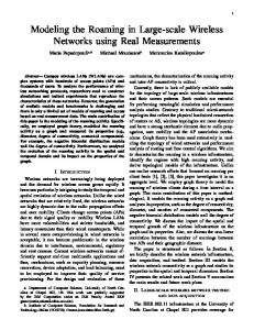
Interfering nodes 2 B out Interfering nodes 2 B in Fig. 1. Illustration of the system model.
II. S YSTEM M ODEL A. System Setup and Key Assumptions We model the locations of transmitting nodes as a uniform-BPP, where a fixed number of nodes are i.i.d. in a finite region A ⊂ R2 . For notational and expositional simplicity, we consider A = b(o, rd ), which is a common assumption in the literature [6]–[9], [12]. Here b(o, rd )
denotes ball of radius rd that is centered at the origin. We assume N t transmitting nodes are independently and uniformly distributed in this ball. Denoting the locations of transmitting nodes by {yi } ≡ Φt , the probability density function (PDF) of each element yi is: 12 kyi k ≤ rd πrd . f (yi ) = 0 otherwise
(1)
It is worth noting that with some work our theoretical results can be extended to the case of arbitrarily-shaped polygon by using the methodology developed in [19]. This is however not in the scope of this paper. We further assume that N a out of N t transmitting (serving and interfering) nodes simultaneously reuse the same resource block. The locations of simultaneously active nodes is denoted by Φa ⊂ Φt . For this setup, we first perform analysis on the reference receiver at an arbitrary location x0 in b(o, rd ) ⊂ R2 . Since uniform-BPP in b(o, rd ) is rotation invariant around the origin, we assume that x-axis is aligned with the location of reference receiver such that x0 = (ν0 , 0), where ν0 = kx0 k ∈ [0, rd ]. We then specialize and extend the analysis of an arbitrarily-located reference receiver to the two cases: i) central receiver, where
6
the reference receiver is located at the center of b(o, rd ), and ii) random receiver, where the reference receiver is chosen uniformly at random amongst set of receiving nodes which are independently and uniformly distributed in b(o, rd ). B. TX-selection Policies and Propagation Model We evaluate the network performance under two generic TX-selection policies: 1) uniform TX-selection policy, where the serving node is chosen uniformly at random from N t transmitting nodes. 2) k-closest TX-selection policy, where the serving node is the k th closest node out of N t transmitting nodes to the reference receiver. These two policies have various applications in ad-hoc and cellular networks. For instance, the special case of k = 1 can be used for modeling and analysis of downlink cellular network and generic k-closest TX-selection policy has several applications to the performance evaluations of emerging paradigms such as cache-enabled networks [17]. More details on the applications of these two policies will be discussed in Section IV. To keep the setup simple, we assume that the background noise is negligible compared to the interference and is hence ignored. Denoting the location of the serving node with y` , the SIR experienced by the reference receiver located at x0 is:
h` kx0 + y` k−α , −α yi ∈Φa \y` hi kx0 + yi k
SIR = P
(2)
where hi ∼ exp(1) and k.k−α model Rayleigh fading and power law path-loss, respectively. It is important to note that after fixing the location of serving node for each policy, the interfering nodes (located at yi ∈ Φa \ y` ⊂ Φt ) are assumed to be chosen uniformly at random amongst set of possible transmitting nodes, i.e., Φt . For a quick reference, we summarize the notation of this paper in Table I. Remark 1 (Scale invariance of BPP network). Since the serving and interfering nodes are chosen from the same point process, the locations of these nodes with respect to the origin get scaled with the same factor when we change rd . This implies that the SIR at the reference receiver located at x0 = (ν0 , 0), where ν0 = κ0 rd and κ0 ∈ [0, 1], is independent of the choice of rd for a given κ0 . Therefore, without loss of generality, we normalize rd to 1. For this setup, we are interested in studying the network performance in terms of coverage probability, which is formally defined next.
7
TABLE I S UMMARY OF NOTATION
Notation
Description
Φt ; N t
Uniform-BPP modeling the locations of transmitting nodes; number of transmitting nodes
Φa ⊆ Φt ; N a
Set of simultaneously active transmitting nodes; number of simultaneously active transmitting nodes
Bin (Bout )
Set of simultaneously active transmitting nodes closer (farther) than serving node to the reference reciver
hi ;α
Channel power gain under Rayleigh fading where hi ∼ exp(1); path loss exponent where α > 2
Pc ; β; NSE (u)
Coverage probability; target SIR; network spectral efficiency
(k)
Coverage probability of an arbitrarily-located reference receiver under uniform TX-selection (k-closest TX-selection) policy
Pcent (Pcent )
(u)
(k)
Coverage probability of a central receiver under uniform TX-selection (k-closest TX-selection) policy
(u) Prand
(k) (Prand )
Coverage probability of a random receiver under uniform TX-selection (k-closest TX-selection) policy
Pref (Pref )
NSE(u) (NSE(k) )
Network spectral efficiency of uniform TX-selection (k-closest TX-selection) policy
PRj ;bj ; Phit
Request probability; caching probability; total hit probability
Definition 1 (Coverage probability). It is defined as the probability that SIR at the reference receiver exceeds the predefined threshold needed to establish a successful connection. Mathematically, it is: Pc = E[1{SIR ≥ β}] = P(SIR ≥ β), where β is the minimum SIR required to establish a successful connection.
III. C OVERAGE P ROBABILITY A NALYSIS This is the first main technical section of the paper, where we evaluate the network performance in terms of coverage probability. Before going into the detailed analysis, we first characterize the distribution of the distances from the reference receiver to the transmitting nodes in the next subsection. This will be a key intermediate result in the coverage analysis. A. Relevant Distance Distributions in a BPP As stated above, the distribution of distances from the interfering and serving nodes hold a key to the derivation of the coverage probability. If the reference receiver is assumed to be located at the origin (i.e., central receiver), it is easy to infer that the sequence of distances from transmitting nodes to the reference receiver which is denoted by {Wi = kyi k} contains i.i.d. elements with PDF and CDF given by [6]: PDF :
fWi (wi ) =
2wi ; rd2
0 ≤ wi ≤ rd ,
CDF :
FWi (wi ) =
wi2 ; rd2
0 ≤ w i ≤ rd .
(3)
However, the sequence of distances from an arbitrarily-located reference receiver, i.e., {Wi = kx0 + yi k}, are correlated due to common factor x0 . This means that if we condition on x0 , the
8
set of distances {Wi = kx0 + yi k}i=1:N t becomes conditionally i.i.d. The conditional CDF and PDF of each element of {Wi }i=1:N t are stated in the next two Lemmas. Lemma 1. The conditional CDF of Wi for a given ν0 = kx0 k is: FWi (wi |ν0 ) F (wi |ν0 ) = w2i2 , 0 ≤ w i ≤ r d − ν0 Wi,1 rd = , F (wi |ν0 ) = wi22 (θ∗ − 1 sin 2θ∗ )+ 1 (φ∗ − 1 sin 2φ∗ ), rd − ν0 < wi ≤ rd + ν0 Wi,2 2 π 2 πr
(4)
d
where θ∗ = arccos
wi2 +ν02 −rd2 2ν0 wi
� , and φ∗ = arccos
ν02 +rd2 −wi2 � . 2ν0 rd
Proof: As noted already, the distances between the transmitting nodes and a reference receiver are independent of coordinates system. Here, we assume that the reference receiver lies on the positive side of x-axis, and hence conditioning on ν0 = kx0 k, instead of x0 suffices. The CDF of FWi (wi |ν0 ) can be derived by using the same geometric argument applied in [20, Theorem 2.3.6]. For completeness the proof is provided in the Appendix A. Lemma 2. The conditional PDF of Wi for a given ν0 is: f (wi |ν0 ) = 2w2i , 0 ≤ wi ≤ rd − ν0 Wi,1 rd fWi (wi |ν0 ) = . � 2 2 2 f (wi |ν0 ) = 2w2i arccos wi +ν0 −rd , rd − ν0 < wi ≤ rd + ν0 Wi,2 2ν0 wi πr
(5)
d
Proof: fWi (wi |ν0 ) can be derived by taking the derivative of FWi (wi |ν0 ) with respect to wi , and using basic algebraic manipulations. It is to be noted that this PDF is also provided in [19]. As discussed above the N t elements of the sequences of distances {Wi = kx0 + yi k}i=1:N t are conditionally i.i.d. with density functions characterized by Lemmas 1 and 2. This i.i.d. property is useful in characterizing the distributions of serving and interfering distances for the two TX-selection policies. We first focus on the distributions of various distances for uniform TX-selection policy, where the serving distance is one the elements of {Wi }i=1:N t that is chosen uniformly at random. The random selection of serving distance infers that the density function of serving distance simply follows that of Wi given by Lemma 2. Denoting the serving distance by R = kx` + yi k, the conditional PDF of serving distance corresponding to the uniform TXselection policy is: (u)
fR (r|ν0 ) = fWi (r|ν0 ).
(6)
9
Similarly, the N a − 1 elements of interfering distances {U = kx0 + yi k, i 6= `} are chosen uniformly at random. Hence the elements of {U } are conditionally i.i.d., where the PDF of each element is: fU (u|ν0 ) = fWi (u|ν0 ),
(7)
where subscript i is dropped for notational simplicity. We now focus on k-closest TX-selection policy, where the serving node is the k th closest node to the reference receiver. Therefore, it is required to “order” the distances from transmitting nodes to the reference receiver to characterize the density functions of serving and interfering distances. We define an ordered set {wi:N t }i=1:N t by sorting the value of wi -s in ascending order such that w1:N t < w2:N t < ... < wN t :N t . Using the conditionally i.i.d. property of {Wi }, the conditional PDF of serving distance R = Wk:N t is: f (k) (r|ν0 ), 0 ≤ r ≤ rd − ν0 R,1 (k) (8) fR (r|ν0 ) = f (k) (r|ν0 ), rd − ν0 < r ≤ rd + ν0 R,2 (k)
with fR,j (r|ν0 ) =
N t! k−1 N t −k (r|ν )) ; j = {1, 2}, (r|ν )(1 − F (r|ν ) f F 0 0 W 0 W W i,j i,j i,j (k − 1)!(N t − k)!
(k)
where, fR (r|ν0 ) can be obtained from the PDF of the k order statistics of the sequence of i.i.d. random variables {Wi }i=1:N t with sampling PDF fWi (wi |ν0 ) [21]. It is important to note that the possible interfering nodes can lie at any place except the location of the serving node. This means that the k th closest transmitting node to the reference receiver is explicitly removed from the interference field. In order to incorporate this in the analysis, we partition the set of distances from active transmitting nodes (located at yi ∈ Φa ) to the random receiver into three
subsets {B in , wk:N t , B out } such that B in and B out represent the set of interfering nodes closer and farther to the reference receiver, respectively, compared to the serving node. This setup is illustrated in Fig. 1. The following Lemma deals with conditional i.i.d. property of Uin ∈ B in and Uout ∈ B out , and their density functions.
Lemma 3. Under k-closest TX-selection policy, the sequences of random variables Uin ∈ B in
and Uout ∈ B out conditioned on r = wk:N t , and ν0 are independent. Moreover,
i) the elements in the sequence of random variables Uin ∈ B in conditioned on r = wk:N t , and
10
ν0 are i.i.d., where the PDF of each element is fUin (uin |ν0 , r) fW (uin |ν0 ) i,1 , 0 < r < w− , 0 < uin < r FWi,1 (r|ν0 ) fWi,1 (uin |ν0 ) fWi (uin |ν0 ) = , w− < r < w+ , 0 < uin < w− , uin < r FWi (r|ν0 ) FWi,2 (r|ν0 ) = , fWi,2 (uin |ν0 ) , w− < r < w+ , w− < u < r in FWi,2 (r|ν0 ) 0, uin ≥ r
(9)
ii) the elements in the sequence of random variables Uout ∈ B out conditioned on r = wk:N t , and ν0 are i.i.d, where the PDF of each element is fUout (uout |ν0 , r) fW (uout |ν0 ) i,1 , 0 < r < w− , r < uout < w− 1−FWi,1 (r|ν0 ) fWi,2 (uout |ν0 ) fWi (uout |ν0 ) = , 0 < r < w− , w− < uout < w+ , uout > r 1−FWi (r|ν0 ) 1−F Wi,1 (r|ν0 ) = , fWi,2 (uout |ν0 ) , w− < r < w+ , r < u < w+ out 1−FWi,2 (r|ν0 ) 0, uout ≤ r
(10)
with w− = rd − ν0 , and w+ = rd + ν0 , where FWi (.|ν0 ), and fWi (.|ν0 ) are given by Lemmas 1 and 2. Proof: See Appendix B. Please note that in [22], [23], we proved similar i.i.d. property for the distribution of distances in Thomas cluster process. B. Laplace transform of interference In this subsection, we characterize the Laplace transform of interference distributions for various choices of intended receiver and transmitter by using the density functions of distances derived in the previous subsection. As will be evident in the sequel, the characterization of Laplace transform of interference distribution is the key intermediate step in the coverage probability analysis. 1) Laplace transform of interference under uniform TX-selection policy: The Laplace transform of interference under uniform TX-selection policy is given in the next Lemma. Lemma 4. Under uniform TX-selection policy, the Laplace transform of interference distribution (u)
conditioned on the location of reference receiver, i.e., ν0 = kx0 k, is LI (s|ν0 ) = �N a −1 � Z rd +ν0 u 2 u2 + ν02 − rd2 � 1 C(α, s, rd − ν0 ) + arccos du , −α πr rd2 2ν0 u d rd −ν0 1 + su
(11)
11
2 2 with C(α, s, x) = x2 − x2 2 F1 (1, , 1 + , −xα /s)), α α P∞ zk Qk−1 (a+l)(b+l) where 2 F1 (a, b; c; z) = 1 + k=1 k! l=0 . c+l
(12)
Proof: See Appendix C The Laplace transform of interference distribution given by Lemma 4 reduces to the simple closed-form expression for the special case of central receiver. This result is presented in the next Corollary and can be readily proved by substituting ν0 = 0 in Lemma 4. Corollary 1. Under uniform TX-selection policy, the Laplace transform of interference at the central receiver is: (u) LI (s)
� =
�N a −1 1 C(α, s, rd ) , rd2
(13)
which for α = 4 simplifies to (u) LI (s)
� �N a −1 √ s rd2 = 1 − 2 arctan √ , rd s
(14)
where C(α, s, rd ) is given by (12). We will use this result to approximate the coverage probability of an arbitrarily-located reference receiver later in this section. 2) Laplace transform of interference under k-closest TX-selection policy: As stated in the previous subsection, the potential interfering nodes can lie at any place except the location of the serving node (i.e., the k th closest node to the reference receiver). We mathematically incorporated this by partitioning the set of distances from interfering nodes to the reference receiver into subsets: B in and B out . In Lemma 3, we formally showed that the sequence of distances Uin ∈ B in and Uout ∈ B out conditioned on the location of the serving node are i.i.d.
Now, using the PDF of distances presented in Lemma 3, the “exact” expression of the Laplace transform of interference distribution at an arbitrarily-located reference receiver is provided in the next Lemma. Lemma 5. Under k-closest TX-selection policy, the Laplace transform of interference conditioned on the location of reference receiver and the serving distance is: A(s, r, ν ), 0 ≤ r ≤ w− 0 (k) LI (s|ν0 , r) = , with B(s, r, ν0 ), w− < r ≤ w+
(15)
12
a
A(s, r, ν0 ) = ×
Z
w−
r
nm X
ξ(p, nam )
0
`=0
fWi,1 (uin |ν0 ) 1 duin −α 1 + suin FWi,1 (r|ν0 )
!`
!N a −`−1 Z w+ fWi,1 (uout |ν0 ) fWi,2 (uout |ν0 ) 1 1 duout + duout , and −α 1 − F 1 + suout −α 1 − FWi,1 (r|ν0 ) Wi,1 (r|ν0 ) w− 1 + suout a
B(s, r, ν0 ) =
where w
r
Z
−
nm X
Z
ξ(p, nam )
0
`=0
= rd − ν0 , w
w−
+
!` Z r fWi,1 (uin |ν0 ) fWi,2 (uin |ν0 ) 1 1 duin + duin −α F 1 + suin −α FWi,2 (r|ν0 ) Wi,2 (r|ν0 ) w− 1 + suin !N a −`−1 Z w+ fWi,1 (uout |ν0 ) 1 duout , × 1 + suout −α 1 − FWi,2 (r|ν0 ) r
= rd + ν0 ,
nam = min(k − 1, N a − 1).
ξ(p, nam )
=
a −`−1 N a −1 ` Pnam ` a N a −`−1 N −1 p (1−p) `=0 `
p` (1−p)N
(
)
(
)
, p =
k−1 , N t −1
and
Proof: See Appendix D. This result can be simplified further for the special case of the central receiver, where it reduces to a simple expression presented in the next Corollary. Corollary 2. The Laplace transform of interference distribution at the central receiver conditioned on the serving distance r = wk:N t is: � �` � �N a −`−1 nam X C(α, s, r) C(α, s, rd ) − C(α, s, r) (k) a ξ(p, nm ) LI (s|r) = , 2 2 2 r r − r d `=0
(16)
where C(α, s, x) is given by (12). Proof: This result can be simply derived by substituting ν0 = 0 in Lemma 5, where the final expression is obtained by using [24, eq (3.194.1)]. This simple expression will be used to characterize the performance of the central receiver and approximate the coverage probability of an arbitrarily-located reference receiver in the next subsection. C. Coverage Probability Using the Laplace transform of interference distributions derived in the previous subsection, we now derive the coverage probability for the two TX-selection polices. We begin our discussion with the uniform TX-selection policy.
13
1) Coverage probability under uniform TX-selection policy: The coverage probability for uniform TX-selection policy is presented in the next Theorem. Theorem 1 (Uniform TX-selection policy). The coverage probability of the reference receiver located at distance ν0 = kx0 k from origin is: Z Z rd −ν0 (u) (u) α LI (βr |ν0 )fWi,1 (r|ν0 )dr + Pref (ν0 ) =
rd +ν0
rd −ν0
0
(u)
LI (βrα |ν0 )fWi,2 (r|ν0 )dr,
(17)
(u)
where fWi,1 (.|ν0 ), fWi,2 (.|ν0 ) are given by Lemma 2, and LI (.|ν0 ) is given by Lemma 4. Proof: Using the definition of coverage probability, we have � X X � (a) h P h` ≥ βrα hi kyi k−α =ER exp − βrα
yi ∈Φa \y`
yi ∈Φa \y`
� i hi kyi k−α R
where (a) follows from h` ∼ exp(1). From this step, the final result can be obtained by using the definition of Laplace transform, followed by de-conditioning over serving distance R. From Theorem 1, two corollaries are in order. First, we specialize the result to the case of central receiver in the next Corollary. This result can be easily proved by substituting ν0 = 0 in Theorem 1, and using Laplace transform of interference distribution given by Corollary 1. Corollary 3 (Uniform TX-selection policy). The coverage probability of the central receiver located at the origin is: (u) Pcent
Z = 0
rd
(u)
LI (βrα )fWi (r)dr,
(18)
(u)
where fWi (.) and LI (.) are given by (3) and (13), respectively. Second, we generalize the result of Theorem 1 to analyze the performance of a random receiver, where the intended receiver is chosen uniformly at random. This result can be simply obtained by de-conditioning the result of Theorem 1 with respect to distance from a randomly chosen receiver to the origin. Now, recall that the receiving nodes are independently and uniformly distributed in b(o, ν0 ), and hence the PDF of distance from a random receiver to the origin is [6]: fV0 (ν0 ) =
2ν0 . rd2
Using this PDF, the coverage probability of a random receiver is stated next.
(19)
14
1
0.38
Na = 5
Na = 4
0.36 Coverage probability
Coverage probability
0.8 N a = 10 0.6 N a = 20 0.4 (u)
0.2
Corollary 4: Prand (u) Corollary 3: Pcent Simulation
0.34
(u)
Theorem 1: Pref (ν0 ) (u)
0.32
Corollary 3: Pcent
0.3 Na = 5
0.28 0.26 0.24
Na = 6 0.22
0 -60
-40
-20 SIR thereshold, β
0
20
0
0.2 0.4 0.6 0.8 Distance from reference receiver to origin, ν0
1
Fig. 2. Coverage probability as a function of SIR threshold
Fig. 3. Coverage probability of reference receiver as a function
(α = 4, and rd = 1).
of its distance to the origin (β = −6 dB, α = 4, and rd = 1).
Corollary 4 (uniform TX-selection policy). The coverage probability of a random receiver is: Z rd (u) (u) Prand = Pref (ν0 )fV0 (ν0 ) dν0 , (20) 0
where
(u) Pref (.)
and fV0 (.) are given by (17) and (19), respectively.
Remark 2. The coverage probability of the central receiver provides an approximation for that of a random receiver. This is because putting the receiver at the center of b(o, rd ) has two conflicting effects on the coverage probability: i) interfering link distances decrease that increase interference power, and ii) serving link distance decreases that increases received power of the desired signal. Depending upon the network parameters and TX-selection policy, one of these effects (increasing interference/ received power) dominates the other. Hence, the approximation provided by central receiver is not strictly a bound ( i.e., lower or upper bounds) of coverage probability of a random receiver. We plot the coverage probability of a random receiver and central receiver as a function of SIR threshold in Fig. 2. The theoretical results of coverage probability under uniform TXselection policy match perfectly with simulation, thereby validating the accuracy of the analysis. As formally stated in Remark 2 and evident from Fig. 2, the coverage probability of the central receiver given by Corollary 3 results in approximation for that of a random receiver. This observation emphasizes on the importance of the accurate random receiver analysis. In order to understand how the performance of the central receiver differs from that of an arbitrarily-
15
1
Increasing k=1,2,3,5.
Coverage probability
0.8
0.6
0.4 (k)
Corollary 6: Prand (k) Corollary 5: Pcent (u) Corollary 4: Prand Simulation
0.2
0 -60
Fig. 4.
-40
-20 0 SIR threshold, β (dB)
Coverage probability as a function of SIR threshold (α = 4, rd = 1, and N a = N t = 5) 0.56
0.8
β = −10 dB 0.54
β = −2 dB
0.75
Coverage probability
Coverage probability
20
0.7 β = 0 dB 0.65
0.6
Theorem 2: Corollary 5:
β = 2 dB
(1) Pref (ν0 ) (1) Pcent
0.2
0.4
0.6
0.8
β = −9 dB
0.5 0.48
β = −8 dB
0.46 0.44 (2)
Theorem 2: Pref (ν0 ) (2) Corollary 5: Pcent
0.42
0.55 0
0.52
1
Distance from reference receiver to origin, ν0
0.4 0
0.2
0.4
0.6
0.8
1
Distance from reference receiver to origin, ν0
Fig. 5. Coverage probability of reference receiver as a function
Fig. 6. Coverage probability of reference receiver as a function
of its distance to the origin (α = 4, rd = 1, and N a = N t = 5)
of its distance to the origin (α = 4, rd = 1, and N a = N t = 5)
located reference receiver, Fig. 3 plots coverage probability of the reference receiver as a function of its distance from origin. In this and the rest of the plots, asterisk will be used to denote the extrema (maximum and minimum) of the curves. As evident from Fig. 3, the coverage probability strongly depends upon the location of the reference receiver. 2) Coverage probability under k-closest TX-selection policy: We now use the Laplace transform of interference distribution derived in Lemma 5 to characterize the coverage probability of an arbitrarily-located reference receiver under k-closest TX-selection policy in the next Theorem. As noted earlier, this result can be specialized to study coverage probability in a cellular network modeled as a finite network (such as in mmWave communications). It can also be used to study
16
several emerging applications in wireless networks. Some examples will be provided in the next Section. Theorem 2 (k-closest TX-selection policy). Using the Laplace transform of interference given by Lemma 5, the coverage probability of the reference receiver located at distance ν0 = kx0 k from origin is: (k) Pref (ν0 )
Z
rd −ν0
A(βr
= 0
α
(k) , r, ν0 )fR,1 (r|ν0 )dr
Z
rd +ν0
+ rd −ν0
(k)
B(βrα , r, ν0 )fR,2 (r|ν0 )dr,
(21)
(k)
where fR,j (.|ν0 ) for j ∈ {1, 2} is given by (8). Proof: The proof follows on the same line as that of Theorem 1. This result is specialized to the case of central receiver in the next Corollary. Corollary 5 (k-closest TX-selection policy). The coverage probability of the central receiver for k-closest TX-selection policy is: Z rd (k) (k) (k) LI (βrα |r)fR (r)dr, Pcent =
(22)
0
with,
(k)
fR (r) = (k)
N t! t FWi (r)k−1 fWi (r)(1 − FWi (r))N −k , t (k − 1)!(N − k)!
(23)
where fWi (.) and LI (.|r) are given by (3) and (16), respectively. We further extend the result of Theorem 2 to characterize the performance of a random receiver. This result is presented in the next Corrolary. Corollary 6 (k-closest TX-selection policy). The coverage probability of a random receiver for k-closest TX-selection policy is: (k) Prand
Z =
rd
(k)
Pref (ν0 )fV0 (ν0 )dν0 ,
(24)
0 (k)
where fV0 (.) and Pref (ν0 ) are given by (19) and (21), respectively. Proof: This result can be simply obtained by taking expectation over the coverage probability of an arbitrarily-located reference receiver given by (21) with respect to the distribution of V0 .
The coverage probabilities of the random and central receivers as a function of SIR threshold are presented in Fig. 4. It is evident that the analytical results presented in Corollaries 5 and 6 match perfectly with simulation, which confirms the accuracy of the analyses. Moreover, it
17
can be seen that the coverage probability of the central receiver leads to an approximation for that of a random receiver. The intuition behind this approximation has been stated in Remark 2. We also plot the coverage probability as a function of distance from reference receiver to the origin in Figs. 5 and 6. It can be observed that the coverage probability strongly depends on the location of the reference receiver, which again confirms the necessity of the “exact” analysis for an arbitrarily-located reference receiver. This analysis can also be used for characterizing the performance of the worst and best case receiver in a finite wireless network. IV. A PPLICATIONS AND D ISCUSSION This is the second main technical section of the paper, where we use the distance distributions and coverage probability results presented in the above section to characterize various classical and currently trending problems related to wireless networks. In particular, we study: i) diversity loss due to SIR correlation under selection combining scheme in a finite network, ii) optimal number of simultaneously active links in a finite network, and iii) optimal geographic caching in a finite network. A. Diversity Loss Due to SIR Correlation Diversity loss due to SIR correlation in multi-antenna communication systems has been studied under different assumptions by modeling the system as infinite PPP in [25]–[28]. In this Section, we demonstrate how the distance distributions derived in subsection III-A can be used to extend these analyses to finite network case. Due to space limitations, we will just study the performance of selection combining under interference correlation, which was presented for infinite PPP case in [25]. As will be evident from the analysis, the same approach can be used to study other communications schemes, such as the automatic repeat request, where instead of combining signal in the spatial domain, it is combined over time domain. We consider the same setup as in the previous two sections with the only difference being that the reference receiver is now assumed to have n > 1 antennas. The (Rayleigh) fading coefficients between transmitting nodes and the reference receiver are assumed to be independent across all links. Despite independent fading, the SIR observed across antennas at the reference receiver is correlated due to the common locations of the transmitting nodes. This correlation makes the analysis of coverage probability under diversity combining schemes challenging.
Before going in to the detailed coverage
analysis, we derive the probability of joint occurrence of success event at all n antennas which
18
will serve as the basis for the coverage probability of selection combining under SIR correlation. Recall that the serving distance was denoted by r, and hence the joint success probability is defined as: Pjoint = P(∩nj=1 SIRj ≥ β) = P(∩nj=1 h`,j > βrα Ij ), where SIRj is the SIR observed at the j th antenna, Ij =
P
yi ∈Φa \y`
(25)
hi,j kx0 + yi k−α and hi
and hi,j are exponential random variables with unit mean (modeling Rayleigh fading). We study the impact of correlation on the coverage probability under selection combining for the two TX-selection policies next. 1) Uniform TX-selection policy: Using the density functions of distances presented in Lemma 2, the joint success probability for uniform TX-selection policy is stated in the next Lemma. Lemma 6. The joint success probability of the reference receiver for uniform TX-selection (u)
policy is Pjoint (ν0 , n) = Z Z rd −ν0 (u) α LIn (βr |ν0 )fWi,1 (r|ν0 )dr +
rd +ν0
rd −ν0
0
(u) LIn (s|ν0 )
(u)
LIn (βrα |ν0 )fWi,2 (r|ν0 )dr, with
(26)
� �n �N t −1 Z rd +ν0 � 1 u2 + ν02 − rd2 � 2u 1 = 2 D(α, s, rd − ν0 , n) + arccos du , rd 1 + su−α π 2ν0 u rd −ν0 α
where D(α, s, x, n) =
2x2 ( xs )n F (n, α2 2+α n 2 1
+ n, 1 + α2 + n, −xα /s)), and fWi,1 (.|ν0 ), fWi,2 (.|ν0 ) are
given by Lemma 2. Proof: See Appendix E We now use the result of Lemma 6 to study the effect of SIR correlation on selection combining scheme where transmission is successful if maxj∈{1,2,..n} SIRj ≥ β. Using inclusion-exclusion principle [25], the coverage probability under selection combining scheme can be equivalently expressed as: PSC = P
max m∈{1,2,..n}
�
SIRm ≥ β = P
∪nm=1
�
SIRm ≥ β =
n X
m+1
(−1)
m=1
� � n P(∩m j=1 SIRj ≥ β). (27) m
This definition can be readily used to characterize the coverage probability of a reference receiver for uniform TX-selection policy under selection combining scheme. The result is formally presented in the next Theorem.
19
Theorem 3 (Uniform TX-selection policy). Using the joint success probability given by (26), the coverage probability of a reference receiver under selection combining scheme is: � � n X (u) (u) m+1 n PSC−corr (ν0 , n) = (−1) Pjoint (ν0 , m), m m=1
(28)
where the probability of the same event, i.e., maxm∈{1,2,..n} SIRm ≥ β under the assumption of independent SIR is: �n (u) (u) PSC−ind (ν0 , n) = 1 − 1 − Pref (ν0 ) ,
(29)
(u)
where Pref (ν0 ) is give by (17). 2) k-closest TX-selection policy: We now use the density functions of distances presented in Lemma 3 to derive the joint success probability of a reference receiver for k-closest TX-selection policy. This result is formally stated in the next Lemma. Lemma 7. Using the PDF of serving distances given by (8), the joint success probability of a (k)
reference receiver for k-closest TX-selection policy is Pjoint (ν0 , n) = Z rd −ν0 Z rd +ν0 (k) (k) α Ajoint (βr , r, ν0 , n)fR,1 (r|ν0 )dr + Bjoint (βrα , r, ν0 , n)fR,2 (r|ν0 )dr, where (30) rd −ν0
0
a
Ajoint (s, r, ν0 , n) = w−
Z
�
r
nm X
ξ(p, nam )
Z r� 0
`=0
1 1 + suout −α
�n
Bjoint (s, r, ν0 , n) = Z +
r
�
w−
1 1 + suin −α
ξ(p, nam )
`=0
�n
�n
fWi,1 (uin |ν0 ) duin FWi,1 (r|ν0 )
!`
!N a −`−1 �n Z w+ � fWi,1 (uout |ν0 ) fWi,2 (uout |ν0 ) 1 duout + duout , 1 − FWi,1 (r|ν0 ) 1 + suout −α 1 − FWi,1 (r|ν0 ) w−
a
nm X
1 1 + suin −α
Z
w−
�
0
fWi,2 (uin |ν0 ) duin FWi,2 (r|ν0 )
!`
1 1 + suin −α Z r
w+
�
�n
fWi,1 (uin |ν0 ) duin FWi,2 (r|ν0 )
1 1 + suout −α
where w− = rd − ν0 , and w+ = rd + ν0 , ξ(p, nam ) = nam = min(k − 1, N a − 1).
�n
fWi,1 (uout |ν0 ) duout 1 − FWi,2 (r|ν0 )
a −`−1 N a −1 ` a p` (1−p)N a −`−1 N `−1
p` (1−p)N Pnam `=0
(
)
(
)
, p =
!N a −`−1
k−1 , N t −1
Proof: The proof follows on the same line as that of Lemma 6 where Ajoint (.) and Bjoint (.) can be derived by using the same argument applied in the proof of Lemma 5, and is hence skipped.
20
0.8
1 0.95
Coverage probability
Coverage probability
0.7 0.6 (u)
Theorem 3: PSC−corr (ν0 , n) (u) Theorem 3: PSC−ind (ν0 , n)
0.5 0.4 0.3 Increasing n=2:5
n=1
0.9 0.85 (k)
Theorem 4: PSC−corr (ν0 , n) (k) Theorem 4: PSC−ind (ν0 , n)
0.8 0.75 Increasing n=2:5 0.7
n=1
0.65 0.6
0.2 0
0.2
0.4
0.6
0.8
1
Distance from reference receiver to origin, ν0
0
0.2
0.4
0.6
0.8
1
Distance from reference receiver to origin, ν0
Fig. 7. Coverage probability of reference receiver as a function
Fig. 8. Coverage probability of reference receiver as a function
of its distance to the origin (α = 4, rd = 1, N a = 5, and
of its distance to the origin (α = 4, rd = 1, N a = N t = 5,
β = −5 dB)
and β = 0 dB)
Now using the result of Lemma 7, the coverage probability of a reference receiver for k-closest TX-selection policy under selection combining scheme is presented next. Theorem 4 (k-closest TX-selection policy). Using the joint success probability given by (30), the coverage probability of a reference receiver under selection combining scheme is: � � n X (k) (k) m+1 n PSC−corr (ν0 , n) = (−1) Pjoint (ν0 , m), m m=1
(31)
where the probability of the event maxm∈{1,2,..n} SIRm ≥ β under the assumption of independent SIR is: �n (k) (k) PSC−ind (ν0 , n) = 1 − 1 − Pref (ν0 ) ,
(32)
(k)
where Pref (ν0 ) is give by (21). In Figs. 7 and 8, we plot the coverage probability under selection combining scheme for uniform TX-selection and k-closest TX-selection policies, respectively. It can be seen that the number of antennas at the receiver, n, the coverage probability of both uniform TX-selection and k-closest TX-selection policies improve. However, due to SIR correlation, the actual gains are much smaller compared to the ones predicted under the independent SIR assumption. This observation emphasizes the importance of the exact characterization of SIR correlation for the performance evaluation of diversity combining techniques. Note that this analysis for finite
21
networks would not have been possible without the new distance distributions and coverage results derived in Section III. B. Maximum Number of Simultaneously Active Links In this subsection, we are interested in evaluating the optimal number of links that must be simultaneously activated in a finite wireless network in the same time frequency resource block. In particular, we study the classical trade-off between aggressive frequency reuse (i.e., more number of simultaneously active links on the same frequency band) and the resulting interference. To study this trade-off, we assume all transmitting nodes employ symbols from a Gaussian codebook for their transmissions, then, the minimum spectral efficiency (SE) of the links conditioned on the successful transmission (i.e., when SIR > β) is log2 (1 + β). Hence, SE can be defined as: SE = E[log2 (1 + β) 1{SIR > β}] = log2 (1 + β) P{SIR > β} bits/s/Hz.
(33)
Using this, network spectral efficiency (NSE), i.e., total number of bits transmitted per unit time per unit bandwidth across the whole network, can be defined as: NSE = N a log2 (1 + β) P{SIR > β} bits/s/Hz.
(34)
It should be noted that the NSE is simply a scaled version of the area spectral efficiency, which is a well known metric used typically in the analysis of infinite networks. The definition of NSE is specialized to our setup in the next Proposition. Proposition 1 (NSE). The total number of bits transmitted per unit time per unit bandwidth for uniform TX-selection policy is: (u)
NSE(u) = N a log2 (1 + β) Prand bits/s/Hz,
(35)
(u)
where Prand is given by (20), and under k-closest TX-selection policy NSE is: (k)
NSE(k) = N a log2 (1 + β) Prand bits/s/Hz,
(36)
(k)
where Prand is given by (24). In Fig. 9, we present NSE as a function of number of simultaneously active links for different values of k. Interestingly, it can be seen that when the distance between random receiver and the serving node decreases, i.e., the value of k is reduced, the “optimal number of simultaneously
22
12
4 3.5
Network spectral efficiency (NSE)
Network spectral efficiency (NSE)
4.5 Increasing k=2:6 Proposition 1: NSE(k)
3 2.5 2 1.5 1 0.5 0
10
Proposition 1: NSE(u) Proposition 1: NSE(1)
8 1 6
0.95 0.9
4
0.85 2 2
4
6
0 5
10
15
20
Number of simultaneously active links, N a
Fig. 9. NSE as a function of number of active links (rd = 1, t
β = 0 dB, α = 4, and N = 20)
5
10
15
20
Number of simultaneously active links, N a
Fig. 10. NSE as a function of number of active links (rd = 1, β = 0 dB, α = 4, and N t = 20)
active links” increases. We also compare NSE of uniform TX-selection and k-closest TX-selection (k=1) policies in Fig. 10. It can be observed that increasing number of simultaneously active links has conflicting effect on NSE of these two policies: NSE for uniform TX-selection policy decreases and NSE for k-closest TX-selection (k = 1) policy increases. C. Optimal Geographic Caching in Finite Wireless Networks In this subsection, we demonstrate the applicability of the tools developed in this paper to the performance analysis of cache-enabled finite networks. For detailed motivation and discussions, please refer to the shorter version of this paper [1], where we studied this setup for the central user case. We consider the same setup as the previous two sections, except that the transmitting nodes are now assumed to have a local cache in which they can store some popular files that may be of interest to the other users. The metric of interest in this study is the total hit probability, which is the probability that the receiver of interest finds its requested content in one of the nodes that is accessible from this receiver. The total hit probability in turn depends upon: (i) request probability, which is the probability with which a particular content is requested by the reference receiver (assumed to be known a priori), (ii) caching probability, which is the probability with which a content is cached at a transmitting node (it depends upon the caching strategy), and (iii) coverage probability that guarantees the minimum SIR for successful reception [17]. Our goal is to maximize the total hit probability. To perform this analysis, we consider a finite library of popular contents C = {c1 , c2 , ..., cJ } with size J , where cj denotes the j th most
23
popular content. For simplicity of exposition, we assume that all the contents have same size, which are normalized to one. We further assume that the transmitting nodes are equipped with cache storage of size mc and hence each node can store at most mc popular contents. Now, denoting the specific set of contents at a generic transmitting node by Ω, the caching probability is: bj = P(cj ∈ Ω), where bj denotes the probability that the content cj is stored at a given transmitting node. To model the content popularity in this system, we use Zipf’s distribution due to its practical relevance [29]. Hence, the request probability for file cj is: j −γ PRj = PJ ; −γ i=1 i
1 ≤ j ≤ J,
(37)
where γ represents the parameter of Zipf’s distribution. Now, the total hit probability can be mathematically expressed as: Phit =
J X
t
PRj
j=1
N X k=1
(k)
Prand (1 − bj )k−1 bj ,
(38)
where (1 − bj )k−1 bj indicates that the closest node with content of interest is the k th closest node to the random receiver. Note that we considered random receiver in this case because by construction, we need a “network-averaged” metric. In other words, the content of interest was not found at (k − 1) closet transmitting nodes to the random receiver. On the same lines as [17], the problem of optimal geographic caching in finite wireless networks can be formulated as: P∗hit
s.t.
= max {bj }
J X j=1
J X
t
PRj
j=1
bj ≤ m c ;
N X k=1
(k)
Prand (1 − bj )k−1 bj
0 ≤ bj ≤ 1 ∀j,
(39)
(40)
(k)
where Prand is the new coverage probability result derived in Corollary 6. The necessity and sufficiency of the constraints given by (40) have already been discussed in [17]. For better understanding of this optimization problem, Fig. 11 plots the total hit probability for the simple setup of J = 2, and mc = 1. It can be seen that by increasing the number of simultaneously active transmitting nodes, N a , the optimal caching probability for the most popular content (i.e., b1 ) moves toward one. This is mainly because increasing N a results in higher interference, which in turn decreases coverage probability. For example when there is only one active node (completely orthogonal channel allocation), coverage probability is equal to one under interference limited regime. Hence, it is optimal to cache the two contents with the same probability, i.e., b1 = b2 =
24
1 Increasing Na = 1 : Nt
0.9 Total hit probability
0.8 0.7 0.6 0.5 0.4 0.3 0.2 0.1 0
0.2 0.4 0.6 0.8 Caching probability for file 1
1
Fig. 11. Total hit probability as a function of caching probability for file 1, where asterisk shows optimal hit probability (J = 2, mc = 1, α = 4, β = 0 dB, γ = 1.2, and N t = 20) (k)
0.5. However, by increasing the number of active transmitting nodes, Prand for k > 1 decreases significantly due to increased interference. As demonstrated in Fig. 11, this makes it optimal to cache the more popular contents more often. Though channel orthogonalization is beneficial in terms of total hit probability, it is not desirable for the network throughput which favors having multiple active links as long as the resulting interference remains acceptable. In order to study the trade-off between the number of active links and the resulting interference, we define throughput as: T∗ = N a P∗hit . Figs. 12 and 13 plot maximum hit probability and throughput versus number of active transmitting nodes, respectively. Interestingly, increasing the number of active nodes has a conflicting effect on the maximum hit probability and the throughput: maximum hit probability decreases and throughput increases. This implies that more nodes can be simultaneously activated if the total hit probability remains within acceptable limits. V. C ONCLUSION In this paper, we developed a comprehensive framework for the performance analysis of finite wireless networks. Modeling the locations of nodes as a uniform BPP, we considered two generic TX-selection policies: i) uniform TX-selection policy: the serving node is chosen uniformly at random amongst the set of transmitting nodes, and ii) k-closest TX-selection policy: the serving node is the k th closest node out of N t transmitting nodes to the reference receiver. For these two policies, we derived “exact” expressions of coverage probability corresponding to an arbitrarilylocated reference receiver, using which we specialized and extended the analyses to several cases
25
10
7.5
0.56
0.9
0.54
0.8
8
0.52 0.5
0.7
Increasing γ = 0 : 0.3 : 1.2
7
Increasing γ = 0 : 0.3 : 1.2
0.48 12
13
Throughput, T∗
Maximum hit probability, P∗hit
1
14
0.6 0.5
6.5 6 12
6
13
14
4
0.4
2 β = −2 dB β = 2 dB
β = −2 dB β = 2 dB
0.3
0
0.2 1
5 10 15 Number of simultaneously active links, N a
20
Fig. 12. Maximum hit probability as a function of number of t
active devices (rd = 1, J = 2, mc = 1, α = 4, and N = 20)
1
5
10
15
20
Number of simultaneously active links, N a Fig. 13. Throughput as a function of number of active devices (rd = 1, J = 2, mc = 1, α = 4, and N t = 20)
of interest. The new set of distance distributions and coverage probability results have numerous application in the performance analyses of various modern and classical wireless systems. For instance, k-closest TX-selection result can be easily specialized to study the performance of finite cellular networks. This case is becoming mainstream with the popularity of mmWave communications. We also discussed three possible applications of our new results. First, we investigated the diversity loss due to SIR correlation in a finite network. Second, we obtained the optimal number of links that can be simultaneously activated to maximize NSE. Third, we evaluated optimal caching probability to maximize the total hit probability in cache-enabled finite networks. This work has many extensions. From modeling perspective, it can be extended to an arbitrary shape (instead of a circle) where the node locations follow a more general distribution. Further, this framework can be extended to analyze Mat´ern cluster process where each finite network form one cluster. From system perspective, it can be used for the performance analysis of indoor communication and hotspots, where the infinite PPP assumption may not be applicable. Finally, these tools can also be extended to study the performance of mmWave communication systems where the receiver of interest may experience interference from a finite number of nodes due to blocking.
26
Serving node
o
o ⌫0
rd
rd
(a)
r
r rd
Case 1
⌫0
Receiver Serving node Interfering nodes 2 B in Interfering nodes 2 B out
Case 3
⌫0
Case 2
(b)
Fig. 14. System model of k-closest TX-selection policy wherein (a) r < rd − ν0 , and in (b) r > rd − ν0 .
A PPENDIX A. Proof of Lemma 1 The derivation of the CDF corresponding to the distances between an arbitrarily-located reference receiver to the transmitting nodes can be partitioned into two parts: a) wi ≤ rd −ν0 , and b) wi ≥ rd − ν0 . First, if wi ≤ rd − ν0 , then FWi,1 (wi |ν0 ) simply is FWi,1 (wi |ν0 ) =
πwi2 . πrd2
Second,
if wi > rd − ν0 , then FWi,2 (wi |ν0 ) is the area of intersection of between the circles x2 + y 2 = rd2 , and (x − ν0 )2 + y 2 = wi2 divided by πrd2 . These circles intersect when x = x∗ =
ν02 +rd2 −wi2 . 2ν0
So,
the CDF of Wi,2 can be written as: Z x∗ p Z rd p i 1 h 2 (1 − ((x − ν0 )/wi ) dx + 2rd 1 − (x/rd )2 dx . FWi,2 (wi |ν0 ) = 2 2wi πrd ν0 −wi x∗ By changing variables (ν0 − x)/wi = cos θ in the first integral and x/rd = cos φ in the second integral, we have � � Z 0 Z θ∗ 1 2 2 (1 − cos 2φ)dφ FWi,2 (wi |ν0 ) = 2 2wi (1 − cos 2θ)dθ − 2rd πrd 0 φ∗ � 1 � = 2 wi2 (θ∗ − 1/2 sin 2θ∗ )+rd2 (φ∗ − 1/2 sin 2φ∗ ) , πrd w2 +ν 2 −r2 � ν 2 +r2 −w2 � where θ∗ = arccos i 2ν00wi d , and φ∗ = arccos 0 2ν0drd i . B. Proof of Lemma 3 The joint PDF of “ordered” subset {wi:N t }i=1:N t conditioned on R = Wk:N t and V0 is: Q t f (w1:N t , ..., wN t :N t |ν0 ) (a) N t ! N i=1 fWi (wi:N t |ν0 ) f (w1:N t , ..., wN t :N t |wk:N t , ν0 ) = = fWk:N t (wk:N t |ν0 ) fWk:N t (wk:N t |ν0 )
27
t
N Y fWi (wi:N t |ν0 ) fWi (wi:N t |ν0 ) t (N − k)! = (k − 1)! , F (wk:N |ν0 ) 1 − FWi (wk:N |ν0 ) i=1 Wi i=k+1 | {z }| {z } k−1 Y
(b)
joint PDF of {Wi:N t }i=1:k−1
joint PDF of {Wi:N t }i=k+1:N t
(k)
where fWk:N t (.|ν0 ) = fR (.|ν0 ). Here (a) follows from definition of the joint PDF of order statistics [21, eqn. (2.10)] with sampling PDF fWi (.|ν0 ) given by (5), and (b) follows from substituting the expression of fWk:N t (.|ν0 ) which is given by (8). The product of joint PDFs in (b) implies that the {Wi:N t }i=1:k and {Wi:N t }i=k+1:N t conditioned on the serving distance R = Wk:N and V0 are independent. The joint PDF of {Wi:N t }i=1:k conditioned on R = Wk:N t and V0 is: f (w1:N t , ..., wk−1:N t |wk:N t , ν0 ) = (k − 1)!
k−1 Y i=1
fWi (wi:N t |ν0 ) . FWi (wk:N t |ν0 )
Note that (k−1)! gives possible permutations of distances from “ordered” subset, {Wi:N t }i=1:k−1 , and doesn’t appear in the joint PDF of “unordered” subset {Wi }i=1:k−1 , that is: f (w1 , ..., wk−1 |wk:N t , ν0 ) =
k−1 Y i=1
fWi (wi |ν0 ) ; wi ≤ wk:N t , FWi (wk:N t |ν0 )
where the product of same functional form of the joint PDF f (w1 , ..., wk−1 |wk:N t , ν0 ) infers that the subset of distances in “unordered” set {Wi }i=1:k−1 are i.i.d. with PDF
fWi (wi |ν0 ) . FWi (wk:N t |ν0 )
Recall
that after fixing the location of serving distance the interfering nodes in B in are chosen uniformly at random. This random selection of the interfering distances infers that the PDF of each element of distance in B in is also
fWi (wi |ν0 ) . FWi (wk:N t |ν0 )
Now, recall that the distribution of serving distance has a
piece-wise form. We denote the distances in “unordered” subset B in by uin , and substitute wk:N t with r. From Fig. 14, it can be seen that there are three cases for the distance of interfering nodes closer than serving node to the reference receiver. •
Case 1: the distances from interfering nodes that are closer than the serving node to the reference receiver, where the serving distance is smaller than rd −ν0 , i.e., uin < r < rd −ν0 .
•
Case 2: the distances from interfering nodes that are closer than the serving node to the reference receiver is less than rd − ν0 and the serving distance is greater than rd − ν0 , i.e., uin < rd − ν0 < r < rd + ν0
•
Case 3: the distances from interfering nodes that are closer than the serving node to the reference receiver and the serving distance are greater than rd − ν0 , i.e., rd − ν0 < uin < r < rd + ν0 .
28
The appropriate pieces of PDF and CDF of Wi (see Lemmas 1 and 2) are chosen according to the ranges of r and uin in each case. Thus, we have
fWi (uin |ν0 ) = FWi (r|ν0 )
fWi,1 (uin |ν0 ) FWi,1 (r|ν0 ) fWi,1 (uin |ν0 ) FWi,2 (r|ν0 ) fWi,2 (uin |ν0 ) FWi,2 (r|ν0 )
0 < r < rd − ν0 , 0 < uin < r
,
, rd − ν0 < r < rd + ν0 , 0 < uin < rd − ν0 , , rd − ν0 < r < rd + ν0 , rd − ν0 < uin < r
where the CDF and PDF of Wi,1 and Wi,2 are given by Lemmas 1 and 2. Similar arguments can be applied for the derivation of fUout (.|ν0 , r). C. Proof of Lemma 4 The conditional Laplace transform of interference is: h � �i h X (u) LI (s|ν0 ) = E exp − s hi kx0 + yi k−α = E yi ∈Φa \y`
" (a)
Y
=E
yi ∈Φa \y` (c)
=
�
2 rd2
1 1 + skx0 + yi k−α
rd −ν0
Z 0
u du + 1 + su−α
Z
#
Z
(b)
Y yi ∈Φa \y`
rd +v0
=
0 rd +ν0
rd −ν0
� �i exp − shi kx0 + yi k−α
1 fU (u|ν0 )du 1 + su−α
!N a −1
u 2 u2 + ν02 − rd2 � arccos du 1 + su−α πrd 2ν0 u
�N a −1 ,
where (a) follows from hi ∼ exp(1), (b) follows from converting Cartesian to polar coordinates using density function of distance given by (7) along with conditional i.i.d. property of U with realization denoted by u = kx0 + yi k, and (c) follows from substituting the density function, fU (u|ν0 ), given by (7). The final result can be obtained by using [24, eq(3.194.1)]. D. Proof of Lemma 5 The Laplace transform of interference conditioned on V0 and R = Wk:N t is: h Y � � Y � �i (k) LI (s|ν0 , r) = E exp − shi uin −α exp shi uout −α uout ∈Bout
uin ∈Bin
h Y (a) =E uin ∈Bin (b)
=
nam
X
×
Z r
Y uout ∈Bout
i 1 1 + suout −α
N a −1 ` � a p)N a −`−1 N `−1
p` (1 − p)N
a −`−1
�
Z
r
1 fU (uin |ν0 , r)duin 1 + suin −α in !N a −`−1
Pnam
p` (1 −
ν0 +rd
1 fU (uout |ν0 , r)duout 1 + suout −α out
`=0
`=0
1 1 + suin −α
0
!`
29
where (a) follows from hi ∼ exp(1), and (b) follows from the fact that uin ∈ B in and uout ∈ B out are conditionally i.i.d. with PDF fUin (.|ν0 , r), and fUout (.|ν0 , r), followed by the fact that number of nodes in Bin is a binary random variable with probability p =
k−1 N t −1
conditioned on total being
less than nam = min(k −1, N a −1). Substituting the PDFs of fUin (.|ν0 , r), and fUout (.|ν0 , r) given by Lemma 1 completes the proof. E. Proof of Lemma 6 According to the definition of joint success probability, we have n i � (a) h Y (u) n α Pjoint (ν0 , n) = P ∩j=1 h`,j > βr Ij = E exp(βrα Ij ) j=1
h =E
Y
n Y
yi ∈Φa \y` j=1
Z
rd −ν0
�
0
−α
α
exp βr hi,j kx0 + yi k
1 1 + βrα u−α
�n
2u du + rd2
Z
" �i (b) =E
Y yi ∈Φa \y`
rd +ν0
rd −ν0
�
1 1 + βrα u−α
�n
�
1 α 1 + βr kx0 + yi k−α
�n #
(c)
��
= ER
�N a −1 � u2 + ν02 − rd2 � 2u arccos du πrd2 2ν0 u
where (a) follows from h`,j ∼ exp(1), (b) follows from expectation over hi,j -s along with the fact hi,j -s are i.i.d., and (c) follows from converting Cartesian to polar coordinates by using the density function of distance given by (7) along with conditional i.i.d. property of u = kx0 + yi k. The first integral of (c) reduces to closed form expression by using [24, eq (3.241.4)] and some algebraic manipulation. The final result is obtained by taking expectation over serving distance. R EFERENCES [1] M. Afshang and H. S. Dhillon, “Optimal geographic caching in finite wireless networks,” in Proc., IEEE International workshop on Signal Processing advances in Wireless Commun. (SPAWC), Jul. 2016, available online: arxiv.org/abs/1603.01921. [2] J. G. Andrews, R. K. Ganti, M. Haenggi, N. Jindal, and S. Weber, “A primer on spatial modeling and analysis in wireless networks,” IEEE Commun. Magazine, vol. 48, no. 11, pp. 156–163, Nov. 2010. [3] H. ElSawy, E. Hossain, and M. Haenggi, “Stochastic geometry for modeling, analysis, and design of multi-tier and cognitive cellular wireless networks: A survey,” IEEE Commun. Surveys and Tutorials, vol. 15, no. 3, pp. 996–1019, 3th quarter 2013. [4] J. G. Andrews, A. K. Gupta, and H. S. Dhillon, “A primer on cellular network analysis using stochastic geometry,” arXiv preprint, Apr. 2016, available online: arxiv.org/abs/1604.03183. [5] M. Haenggi, Stochastic Geometry for Wireless Networks.
Cambridge University Press, 2012.
[6] S. Srinivasa and M. Haenggi, “Distance distributions in finite uniformly random networks: Theory and applications,” IEEE Trans. on Vehicular Technology, vol. 59, no. 2, pp. 940–949, 2010. [7] D. Torrieri and M. C. Valenti, “The outage probability of a finite ad hoc network in nakagami fading,” IEEE Trans. on Commun., vol. 60, no. 11, pp. 3509–3518, 2012.
30
[8] K. Venugopal, M. C. Valenti, and R. W. Heath, “Interference in finite-sized highly dense millimeter wave networks,” in Information Theory and Applications Workshop (ITA), 2015, pp. 175–180. [9] ——, “Analysis of millimeter wave networked wearables in crowded environments,” in Proc., IEEE Asilomar, Nov. 2015, pp. 872–876. [10] J. Guo, S. Durrani, and X. Zhou, “Outage probability in arbitrarily-shaped finite wireless networks,” IEEE Trans. on Commun., vol. 62, no. 2, pp. 699–712, 2014. [11] ——, “Performance analysis of arbitrarily-shaped underlay cognitive networks: Effects of secondary user activity protocols,” IEEE Trans. on Commun., vol. 63, no. 2, pp. 376–389, 2015. [12] M. C. Valenti, D. Torrieri, and S. Talarico, “A direct approach to computing spatially averaged outage probability,” IEEE Commun. Letters, vol. 18, no. 7, pp. 1103–1106, 2014. [13] V. V. Chetlur Ravi and H. S. Dhillon, “Downlink coverage probability in a finite network of unmanned aerial vehicle (UAV) base stations,” in Proc., IEEE SPAWC, Jul. 2016. [14] J. G. Andrews, F. Baccelli, and R. K. Ganti, “A tractable approach to coverage and rate in cellular networks,” IEEE Trans. on Commun., vol. 59, no. 11, pp. 3122–3134, 2011. [15] S. Banani, A. Eckford, and R. Adve, “Analyzing the impact of access point density on the performance of finite-area networks,” IEEE Trans. on Commun., vol. 63, no. 12, pp. 5143–5161, 2015. [16] J. Schloemann, H. Dhillon, and R. M. Buehrer, “Towards a tractable analysis of localization fundamentals in cellular networks,” to appear, IEEE Trans. on Wireless Commun., 2015, available online: arxiv.org/abs/1502.06899. [17] B. Błaszczyszyn and A. Giovanidis, “Optimal geographic caching in cellular networks,” in Proc., IEEE Intl. Conf. on Commun. (ICC), 2015. [18] H. P. Keeler, B. Błaszczyszyn, and M. K. Karray, “SINR-based k-coverage probability in cellular networks with arbitrary shadowing,” in Proc., IEEE Intl. Symposium on Information Theory (ISIT), Jul. 2013, pp. 1167–1171. [19] Z. Khalid and S. Durrani, “Distance distributions in regular polygons,” IEEE Trans on Vehicular Technology, vol. 62, no. 5, pp. 2363–2368, 2013. [20] A. M. Mathai, An introduction to geometrical probability: distributional aspects with applications.
Philadelphia, PA,
USA: Gordon and Breach, 1999, vol. 1. [21] M. Ahsanullah and V. B. Nevzorov, Order Statistics: Examples and Exercises.
New York: Nova Science, 2005.
[22] M. Afshang, H. S. Dhillon, and P. H. J. Chong, “Modeling and performance analysis of clustered device-to-device networks,” to appear IEEE Trans. on Wireless Commun., available online: arxiv.org/abs/1508.02668. [23] ——, “Fundamentals of cluster-centric content placement in cache-enabled device-to-device networks,” to appear IEEE Trans. on Commun., 2015, available online: arxiv.org/abs/1509.04747. [24] D. Zwillinger, Table of integrals, series, and products.
Elsevier, 2014.
[25] M. Haenggi, “Diversity loss due to interference correlation,” IEEE Commun. Letters, vol. 16, no. 10, pp. 1600–1603, 2012. [26] R. Tanbourgi, H. S. Dhillon, J. G. Andrews, and F. K. Jondral, “Effect of spatial interference correlation on the performance of maximum ratio combining,” IEEE Transactions on Wireless Communications, vol. 13, no. 6, pp. 3307–3316, Jun. 2014. [27] R. Tanbourgi and F. K. Jondral, “Analysis of heterogeneous cellular networks under frequency diversity and interference correlation,” IEEE Wireless Communications Letters, vol. 4, no. 1, pp. 2–5, Feb. 2015. [28] R. Tanbourgi, H. S. Dhillon, and F. K. Jondral, “Analysis of joint transmit-receive diversity in downlink MIMO heterogeneous cellular networks,” IEEE Trans. on Wireless Commun., vol. 14, no. 12, pp. 6695–6709, Dec. 2015. [29] M. Cha, H. Kwak, P. Rodriguez, Y.-Y. Ahn, and S. Moon, “I Tube, You Tube, Everybody Tubes: analyzing the world’s largest user generated content video system,” in Proc., ACM Intl. Conf. on Special Interest Group on Data Commun. (SIGCOMM), 2007.