Fundamentals of Turbo Codes - Pearsoncmg.com

Fundamentals of Turbo Codes by Bernard Sklar Introduction Concatenated coding schemes were first proposed by Forney [1] as a method for achieving large coding gains by combining two or more relatively simple buildingblock or component codes (sometimes called constituent codes). The resulting codes had the error-correction capability of much longer codes, and they were endowed with a structure that permitted relatively easy to moderately complex decoding. A serial concatenation of codes is most often used for power-limited systems such as transmitters on deep-space probes. The most popular of these schemes consists of a Reed-Solomon outer (applied first, removed last) code followed by a convolutional inner (applied last, removed first) code [2]. A turbo code can be thought of as a refinement of the concatenated encoding structure plus an iterative algorithm for decoding the associated code sequence. Turbo codes were first introduced in 1993 by Berrou, Glavieux, and Thitimajshima, and reported in [3, 4], where a scheme is described that achieves a -5 bit-error probability of 10 using a rate 1/2 code over an additive white Gaussian noise (AWGN) channel and BPSK modulation at an Eb/N0 of 0.7 dB. The codes are constructed by using two or more component codes on different interleaved versions of the same information sequence. Whereas, for conventional codes, the final step at the decoder yields hard-decision decoded bits (or, more generally, decoded symbols), for a concatenated scheme such as a turbo code to work properly, the decoding algorithm should not limit itself to passing hard decisions among the decoders. To best exploit the information learned from each decoder, the decoding algorithm must effect an exchange of soft decisions rather than hard decisions. For a system with two component codes, the concept behind turbo decoding is to pass soft decisions from the output of one decoder to the input of the other decoder, and to iterate this process several times so as to produce more reliable decisions.

Likelihood Functions The mathematical foundations of hypothesis testing rest on Bayes’ theorem. For communications engineering, where applications involving an AWGN channel are of great interest, the most useful form of Bayes’ theorem expresses the a posteriori

probability (APP) of a decision in terms of a continuous-valued random variable x in the following form: P (d = i | x) =

p ( x | d = i ) P (d = i) p ( x)

i = 1 ,..., M

(1)

and p( x ) =

M

∑ i=1

p ( x | d = i ) P (d = i )

(2)

where P(d = i|x) is the APP, and d = i represents data d belonging to the ith signal class from a set of M classes. Further, p(x|d = i) represents the probability density function (pdf) of a received continuous-valued data-plus-noise signal x, conditioned on the signal class d = i. Also, P(d = i), called the a priori probability, is the probability of occurrence of the ith signal class. Typically x is an “observable” random variable or a test statistic that is obtained at the output of a demodulator or some other signal processor. Therefore, p(x) is the pdf of the received signal x, yielding the test statistic over the entire space of signal classes. In Equation (1), for a particular observation, p(x) is a scaling factor, since it is obtained by averaging over all the classes in the space. Lowercase p is used to designate the pdf of a continuous-valued random variable, and uppercase P is used to designate probability (a priori and APP). Determining the APP of a received signal from Equation (1) can be thought of as the result of an experiment. Before the experiment, there generally exists (or one can estimate) an a priori probability P(d = i). The experiment consists of using Equation (1) for computing the APP, P(d = i|x), which can be thought of as a “refinement” of the prior knowledge about the data, brought about by examining the received signal x.

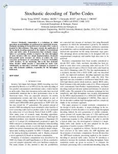
The Two-Signal Class Case Let the binary logical elements 1 and 0 be represented electronically by voltages +1 and -1, respectively. The variable d is used to represent the transmitted data bit, whether it appears as a voltage or as a logical element. Sometimes one format is more convenient than the other; the reader should be able to recognize the difference from the context. Let the binary 0 (or the voltage value -1) be the null element under addition. For signal transmission over an AWGN channel, Figure 1 shows the conditional pdfs referred to as likelihood functions. The rightmost function, p(x|d = +1), shows the pdf of the random variable x conditioned on d = +1 being transmitted. The leftmost function, p(x|d = -1), illustrates a similar pdf conditioned on d = -1 being transmitted. The abscissa represents the full range of 2

Fundamentals of Turbo Codes

possible values of the test statistic x generated at the receiver. In Figure 1, one such arbitrary value xk is shown, where the index denotes an observation in the kth time interval. A line subtended from xk intercepts the two likelihood functions, yielding two likelihood values ℓ1 = p(xk|dk = +1) and ℓ2 = p(xk|dk = -1). A well-known harddecision rule, known as maximum likelihood, is to choose the data dk = +1 or dk = -1 associated with the larger of the two intercept values, ℓ1 or ℓ2, respectively. For each data bit at time k, this is tantamount to deciding that dk = +1 if xk falls on the right side of the decision line labeled γ0, otherwise deciding that dk = -1.

Figure 1 Likelihood functions.

A similar decision rule, known as maximum a posteriori (MAP), which can be shown to be a minimum probability of error rule, takes into account the a priori probabilities of the data. The general expression for the MAP rule in terms of APPs is as follows: H1 > P ( d = +1| x ) P ( d = − 1| x ) < H2

(3)

Equation (3) states that you should choose the hypothesis H1, (d = +1), if the APP P(d = +1|x), is greater than the APP P(d = -1|x). Otherwise, you should choose hypothesis H2, (d = -1). Using the Bayes’ theorem of Equation (1), the APPs in Equation (3) can be replaced by their equivalent expressions, yielding the following: H1 > p ( x | d = +1) P ( d = +1) p ( x | d = − 1) P (d = − 1) < H2 Fundamentals of Turbo Codes

(4)

3

where the pdf p(x) appearing on both sides of the inequality in Equation (1) has been canceled. Equation (4) is generally expressed in terms of a ratio, yielding the so-called likelihood ratio test, as follows: H1 p ( x | d = +1) > P ( d = − 1) p ( x | d = +1) P ( d = +1) or p ( x | d = − 1) < P ( d = +1) p ( x | d = − 1) P ( d = − 1) H2

H1 > 1 < H2

(5)

Log-Likelihood Ratio By taking the logarithm of the likelihood ratio developed in Equations (3) through (5), we obtain a useful metric called the log-likelihood ratio (LLR). It is a real number representing a soft decision out of a detector, designated by as follows:  P ( d = +1| x )   p ( x | d = +1) P ( d = +1)  L( d | x ) = log   = log    P ( d = − 1| x )   p ( x | d = − 1) P ( d = − 1) 

(6)

 p ( x | d = +1)   P ( d = +1)  L( d | x ) = log   + log    p ( x | d = − 1)   P ( d = − 1) 

(7)

L( d | x ) = L( x | d ) + L( d )

(8)

where L(x|d) is the LLR of the test statistic x obtained by measurements of the channel output x under the alternate conditions that d = +1 or d = -1 may have been transmitted, and L(d) is the a priori LLR of the data bit d. To simplify the notation, Equation (8) is rewritten as follows: L′( dˆ ) = Lc( x ) + L( d )

(9)

where the notation Lc(x) emphasizes that this LLR term is the result of a channel measurement made at the receiver. Equations (1) through (9) were developed with only a data detector in mind. Next, the introduction of a decoder will typically yield decision-making benefits. For a systematic code, it can be shown [3] that the LLR (soft output) L( dˆ ) out of the decoder is equal to Equation 10: L( dˆ ) = L′( dˆ ) + Le( dˆ )

4

(10)


where L′( dˆ ) is the LLR of a data bit out of the demodulator (input to the decoder), and Le( dˆ ) , called the extrinsic LLR, represents extra knowledge gleaned from the decoding process. The output sequence of a systematic decoder is made up of values representing data bits and parity bits. From Equations (9) and (10), the output LLR L( dˆ ) of the decoder is now written as follows: L( dˆ ) = Lc( x ) + L(d ) + Le( dˆ )

(11)

Equation (11) shows that the output LLR of a systematic decoder can be represented as having three LLR elements—a channel measurement, a priori knowledge of the data, and an extrinsic LLR stemming solely from the decoder. To yield the final L( dˆ ) , each of the individual LLRs can be added as shown in Equation (11), because the three terms are statistically independent [3, 5]. This soft decoder output L( dˆ ) is a real number that provides a hard decision as well as the reliability of that decision. The sign of L( dˆ ) denotes the hard decision; that is, for positive values of L( dˆ ) decide that d = +1, and for negative values decide that d = -1. The magnitude of L( dˆ ) denotes the reliability of that decision. Often, the value of Le( dˆ ) due to the decoding has the same sign as Lc(x) + L(d), and therefore acts to improve the reliability of L( dˆ ) .

Principles of Iterative (Turbo) Decoding In a typical communications receiver, a demodulator is often designed to produce soft decisions, which are then transferred to a decoder. The error-performance improvement of systems utilizing such soft decisions compared to hard decisions are typically approximated as 2 dB in AWGN. Such a decoder could be called a soft input/hard output decoder, because the final decoding process out of the decoder must terminate in bits (hard decisions). With turbo codes, where two or more component codes are used, and decoding involves feeding outputs from one decoder to the inputs of other decoders in an iterative fashion, a hard-output decoder would not be suitable. That is because hard decisions into a decoder degrades system performance (compared to soft decisions). Hence, what is needed for the decoding of turbo codes is a soft input/soft output decoder. For the first decoding iteration of such a soft input/soft output decoder, illustrated in Figure 2, we generally assume the binary data to be equally likely, yielding an initial a priori LLR value of L(d) = 0 for the third term in Equation (7). The channel LLR value,


5

Lc(x), is measured by forming the logarithm of the ratio of the values of ℓ1 and ℓ2 for a particular observation of x (see Figure 1), which appears as the second term in Equation (7). The output L( dˆ ) of the decoder in Figure 2 is made up of the LLR from the detector, L′( dˆ ) , and the extrinsic LLR output, Le( dˆ ) , representing knowledge gleaned from the decoding process. As illustrated in Figure 2, for iterative decoding, the extrinsic likelihood is fed back to the decoder input, to serve as a refinement of the a priori probability of the data for the next iteration.

Figure 2 Soft input/soft output decoder (for a systematic code).

Log-Likelihood Algebra To best explain the iterative feedback of soft decoder outputs, the concept of loglikelihood algebra [5] is introduced. For statistically independent data d, the sum of two log-likelihood ratios (LLRs) is defined as follows: L(d1) ⊞ L(d2) L L(d1

 e L ( d 1) + e L ( d 2 )  = ) log ⊕ d2 e L ( d 1) L ( d 2 )  e 1 + e 

≈ (-1) × sgn [L(d1)] × sgn [L(d2)] × min (| L(d1) |, | L(d2) |)

6

(12) (13)


where the natural logarithm is used, and the function sign () represents “the polarity of.” There are three addition operations in Equation (12). The + sign is used for ordinary addition. The ⊕ sign is used to denote the modulo-2 sum of data expressed as binary digits. The ⊞ sign denotes log-likelihood addition or, equivalently, the mathematical operation described by Equation (12). The sum of two LLRs denoted by the operator ⊞ is defined as the LLR of the modulo-2 sum of the underlying statistically independent data bits [5]. Equation (13) is an approximation of Equation (12) that will prove useful later in a numerical example. The sum of LLRs as described by Equations (12) or (13) yields the following interesting results when one of the LLRs is very large or very small: L(d) ⊞ ∞ = -L(d) and L(d) ⊞ 0 = 0 Note that the log-likelihood algebra described here differs slightly from that used in [5] because of a different choice of the null element. In this treatment, the null element of the binary set (1, 0) has been chosen to be 0.

Product Code Example Consider the two-dimensional code (product code) depicted in Figure 3. The configuration can be described as a data array made up of k1 rows and k2 columns. The k1 rows contain codewords made up of k2 data bits and n2 - k2 parity bits. Thus, each row (except the last one) represents a codeword from an (n2, k2) code. Similarly, the k2 columns contain codewords made up of k1 data bits and n1 - k1 parity bits. Thus, each column (except the last one) represents a codeword from an n1, k1 code. The various portions of the structure are labeled d for data, ph for horizontal parity (along the rows), and pv for vertical parity (along the columns). In effect, the block of k1 x k2 data bits is encoded with two codes—a horizontal code, and a vertical code. Additionally, in Figure 3, there are blocks labeled Leh and Lev that contain the extrinsic LLR values learned from the horizontal and vertical decoding steps, respectively. Error-correction codes generally provide some improved performance. We will see that the extrinsic LLRs represent a measure of that improvement. Notice that this product code is a simple example of a concatenated code. Its structure encompasses two separate encoding steps—horizontal and vertical.


7

Figure 3 Product code.

Recall that the final decoding decision for each bit and its reliability hinges on the value of L( dˆ ) , as shown in Equation (11). With this equation in mind, an algorithm yielding the extrinsic LLRs (horizontal and vertical) and a final L( dˆ ) can be described. For the product code, this iterative decoding algorithm proceeds as follows: 1.

Set the a priori LLR L(d) = 0 (unless the a priori probabilities of the data bits are other than equally likely).

2.

Decode horizontally, and using Equation (11) obtain the horizontal extrinsic LLR as shown below: Leh( dˆ ) = L ( dˆ ) − Lc( x ) − L ( d )

3.

Set L ( d ) = Leh( dˆ ) for the vertical decoding of step 4.

4.

Decode vertically, and using Equation (11) obtain the vertical extrinsic LLR as shown below:

Lev ( dˆ ) = L ( dˆ ) − Lc ( x ) − L ( d )

8


5.

Set L ( d ) = Lev( dˆ ) and repeat steps 2 through 5.

6.

After enough iterations (that is, repetitions of steps 2 through 5) to yield a reliable decision, go to step 7.

7.

The soft output is L ( dˆ ) = Lc ( x ) + Leh ( dˆ ) + Lev ( dˆ )

(14)

An example is next used to demonstrate the application of this algorithm to a very simple product code.

Two-Dimensional Single-Parity Code Example At the encoder, let the data bits and parity bits take on the values shown in Figure 4(a), where the relationships between data and parity bits within a particular row (or column) expressed as the binary digits (1, 0) are as follows: di ⊕ dj = pij di = dj ⊕ pij

i, j = 1, 2

(15) (16)

where ⊕ denotes modulo-2 addition. The transmitted bits are represented by the sequence d1 d2 d3 d4 p12 p34 p13 p24. At the receiver input, the noise-corrupted bits are represented by the sequence {xi}, {xij}, where xi = di + n for each received data bit, xij = pij + n for each received parity bit, and n represents the noise contribution that is statistically independent for both di and pij. The indices i and j represent position in the encoder output array shown in Figure 4(a). However, it is often more useful to denote the received sequence as {xk}, where k is a time index. Both conventions will be followed below—using i and j when focusing on the positional relationships within the product code, and using k when focusing on the more general aspect of a time-related signal. The distinction as to which convention is being used should be clear from the context. Using the relationships developed in Equations (7) through (9), and assuming an AWGN interference model, the LLR for the channel measurement of a signal xk received at time k is written as follows:  p ( x k | d k = +1)    p ( x k | d k = − 1) 

Lc ( x k ) = loge 


(17a)

9

2   1 1  xk − 1     exp −    σ 2π  2 σ     = loge  2  1 1  xk + 1     exp −    σ 2π  2 σ      2

       

(17b)

2

1 1  xk + 1  2 − 1 = −  xk  +   = 2 xk 2 σ  2 σ  σ

(17c)

where the natural logarithm is used. If a further simplifying assumption is made that the noise variance is σ2 is unity, then Lc(xk) = 2xk

(18)

Consider the following example, where the data sequence d1 d2 d3 d4 is made up of the binary digits 1 0 0 1, as shown in Figure 4. By the use of Equation (15), it is seen that the parity sequence p12 p34 p13 p24 must be equal to the digits 1 1 1 1. Thus, the transmitted sequence is {di}, {pij} = 1 0 0 1 1 1 1 1

(19)

When the data bits are expressed as bipolar voltage values of +1 and -1 corresponding to the binary logic levels 1 and 0, the transmitted sequence is {di}, {pij} = +1 -1 -1 +1 +1 +1 +1 +1 Assume now that the noise transforms this data-plus-parity sequence into the received sequence {xi}, {xij} = 0.75, 0.05, 0.10, 0.15, 1.25, 1.0, 3.0, 0.5

(20)

where the members of {xi}, {xij} positionally correspond to the data and parity {di}, {pij} that was transmitted. Thus, in terms of the positional subscripts, the received sequence can be denoted as {xi}, {xij} = x1, x2, x3, x4, x12, x34, x13, x24 From Equation (18), the assumed channel measurements yield the LLR values {Lc(xi)}, {Lc(xij)} = 1.5, 0.1, 0.20, 0.3, 2.5, 2.0, 6.0, 1.0

10

(21)


These values are shown in Figure 4b as the decoder input measurements. It should be noted that, given equal prior probabilities for the transmitted data, if hard decisions are made based on the {xk} or the {Lc(xk)} values shown above, such a process would result in two errors, since d2 and d3 would each be incorrectly classified as binary 1.

Figure 4 Product code example.

Extrinsic Likelihoods For the product-code example in Figure 4, we use Equation (11) to express the soft output L ( dˆ1) for the received signal corresponding to data d1, as follows.

L ( dˆ1) = Lc ( x1) + L ( d 1) + {[ Lc ( x 2) + L ( d 2)]

⊞ Lc( x12)}

(22)

where the terms {[Lc(x2) + L(d2)] ⊞ Lc(x12)} represent the extrinsic LLR contributed by the code (that is, the reception corresponding to data d2 and its a priori probability, in conjunction with the reception corresponding to parity p12). In general, the soft output L ( dˆ i ) for the received signal corresponding to data di is

L ( dˆ i ) = Lc ( xi ) + L ( d i ) + {[ Lc ( x j ) + L ( d j )]

⊞ Lc( xij )}

(23)

where Lc(xi), Lc(xj), and Lc(xij) are the channel LLR measurements of the reception corresponding to di, dj, and pij, respectively. L(di) and L(dj) are the LLRs of the a priori probabilities of di and dj, respectively, and {[Lc(xj) + L(dj)] ⊞ Lc(xij)} is the


11

extrinsic LLR contribution from the code. Equations (22) and (23) can best be understood in the context of Figure 4b. For this example, assuming equally-likely signaling, the soft output L ( dˆ1) is represented by the detector LLR measurement of

Lc(x1) = 1.5 for the reception corresponding to data d1, plus the extrinsic LLR of [Lc(x2) = 0.1] ⊞ [Lc(x12) = 2.5] gleaned from the fact that the data d2 and the parity p12 also provide knowledge about the data d1, as seen from Equations (15) and (16).

Computing the Extrinsic Likelihoods For the example in Figure 4, the horizontal calculations for Leh( dˆ ) and the vertical calculations for Lev( dˆ ) are expressed as follows: Leh ( dˆ1 ) = [ Lc ( x2 ) + L ( dˆ2 )] ⊞ Lc ( x12 )

(24a)

Lev ( dˆ1 ) = [ Lc ( x3 ) + L ( dˆ3 )] ⊞ Lc ( x13 )

(24b)

Leh ( dˆ2 ) = [ Lc ( x1 ) + L ( dˆ1 )] ⊞ Lc ( x12 )

(25a)

Lev ( dˆ2 ) = [ Lc ( x4 ) + L ( dˆ4 )] ⊞ Lc ( x24 )

(25b)

Leh ( dˆ3 ) = [ Lc ( x4 ) + L ( dˆ4 )] ⊞ Lc ( x34 )

(26a)

Lev ( dˆ3 ) = [ Lc ( x1 ) + L ( dˆ1 )] ⊞ Lc ( x13 )

(26b)

Leh ( dˆ4 ) = [ Lc ( x3 ) + L ( dˆ3 )] ⊞ Lc ( x34 )

(27a)

Lev ( dˆ4 ) = [ Lc ( x2 ) + L ( dˆ2 )] ⊞ Lc ( x24 )

(27b)

The LLR values shown in Figure 4 are entered into the Leh( dˆ ) expressions in Equations (24) through (27) and, assuming equally-likely signaling, the L(d) values are initially set equal to zero, yielding

12

Leh( dˆ1) = (0.1 + 0) ⊞ 2.5 ≈ − 0.1 = new L( d 1)

(28)

Leh( dˆ 2) = (1.5 + 0) ⊞ 2.5 ≈ − 1.5 = new L ( d 2)

(29)


Leh( dˆ 3) = (0.3 + 0) ⊞ 2.0 ≈ − 0.3 = new L ( d 3)

(30)

Leh( dˆ 4) = (0.2 + 0) ⊞ 2.0 ≈ − 0.2 = new L ( d 4)

(31)

where the log-likelihood addition has been calculated using the approximation in Equation (13). Next, we proceed to obtain the first vertical calculations using the Lev( dˆ ) expressions in Equations (24) through (27). Now, the values of L(d) can be refined by using the new L(d) values gleaned from the first horizontal calculations, shown in Equations (28) through (31). That is,

Lev( dˆ1) = (0.2 − 0.3) ⊞ 6.0 ≈ 0.1 = new L ( d 1)

(32)

Lev( dˆ 2) = (0.3 − 0.2) ⊞ 1.0 ≈ − 0.1 = new L ( d 2)

(33)

Lev( dˆ 3) = (1.5 − 0.1) ⊞ 6.0 ≈ − 1.4 = new L ( d 3)

(34)

Lev( dˆ 4) = (0.1 − 1.5) ⊞ 1.0 ≈ 1.0 = new L ( d 4)

(35)

The results of the first full iteration of the two decoding steps (horizontal and vertical) are shown below. Original Lc(xk) measurements 1.5

0.1

-0.1

-1.5

0.2

0.3

-0.3

-0.2

Leh( dˆ ) after first horizontal decoding 0.1

-0.1

-1.4

1.0

Lev( dˆ ) after first vertical decoding Each decoding step improves the original LLRs that are based on channel measurements only. This is seen by calculating the decoder output LLR using


13

Equation (14). The original LLR plus the horizontal extrinsic LLRs yields the following improvement (the extrinsic vertical terms are not yet being considered): Improved LLRs due to Leh( dˆ ) 1.4

-1.4

-0.1

0.1

The original LLR plus both the horizontal and vertical extrinsic LLRs yield the following improvement: Improved LLRs due to Leh( dˆ ) + Lev( dˆ ) 1.5

-1.5

-1.5

1.1

For this example, the knowledge gained from horizontal decoding alone is sufficient to yield the correct hard decisions out of the decoder, but with very low confidence for data bits d3 and d4. After incorporating the vertical extrinsic LLRs into the decoder, the new LLR values exhibit a higher level of reliability or confidence. Let’s pursue one additional horizontal and vertical decoding iteration to determine if there are any significant changes in the results. We again use the relationships shown in Equations (24) through (27) and proceed with the second horizontal calculations for Leh( dˆ ) , using the new L(d) from the first vertical calculations shown in Equations (32) through (35), so that

Leh( dˆ1) = (0.1 − 0.1) ⊞ 2.5 ≈ 0 = new L ( d 1)

(36)

Leh( dˆ 2) = (1.5 + 0.1) ⊞ 2.5 ≈ − 1.6 = new L ( d 2)

(37)

Leh( dˆ 3) = (0.3 + 1.0) ⊞ 2.0 ≈ − 1.3 = new L ( d 3)

(38)

Leh( dˆ 4) = (0.2 − 1.4) ⊞ 2.0 ≈ 1.2 = new L ( d 4)

(39)

Next, we proceed with the second vertical calculations for Lev( dˆ ) , using the new L(d) from the second horizontal calculations, shown in Equations (36) through (39). This yields

14


Lev( dˆ1) = (0.2 − 1.3) ⊞ 6.0 ≈ 1.1 = new L ( d 1)

(40)

Lev( dˆ 2) = (0.3 + 1.2) ⊞ 1.0 ≈ − 1.0 = new L ( d 2)

(41)

Lev( dˆ 3) = (1.5 + 0) ⊞ 6.0 ≈ − 1.5 = new L ( d 3)

(42)

Lev( dˆ 4) = (0.1 − 1.6) ⊞ 1.0 ≈ 1.0 = new L ( d 4)

(43)

The second iteration of horizontal and vertical decoding yielding the above values results in soft-output LLRs that are again calculated from Equation (14), which is rewritten below: L ( dˆ ) = Lc( x ) + Leh( dˆ ) + Lev( dˆ )

(44)

The horizontal and vertical extrinsic LLRs of Equations (36) through (43) and the resulting decoder LLRs are displayed below. For this example, the second horizontal and vertical iteration (yielding a total of four iterations) suggests a modest improvement over a single horizontal and vertical iteration. The results show a balancing of the confidence values among each of the four data decisions. Original Lc(x) measurements 1.5

0.1

0

-1.6

0.2

0.3

-1.3

1.2

Leh( dˆ ) after second horizontal decoding 1.1

-1.0

-1.5

1.0

Lev( dˆ ) after second vertical decoding The soft output is L ( dˆ ) = Lc( x ) + Leh( dˆ ) + Lev( dˆ )


15

which after a total of four iterations yields the values for L( dˆ ) of 2.6

-2.5

-2.6

2.5

Observe that correct decisions about the four data bits will result, and the level of confidence about these decisions is high. The iterative decoding of turbo codes is similar to the process used when solving a crossword puzzle. The first pass through the puzzle is likely to contain a few errors. Some words seem to fit, but when the letters intersecting a row and column do not match, it is necessary to go back and correct the first-pass answers.

Encoding with Recursive Systematic Codes The basic concepts of concatenation, iteration, and soft-decision decoding using a simple product-code example have been described. These ideas are next applied to the implementation of turbo codes that are formed by the parallel concatenation of component convolutional codes [3, 6]. A short review of simple binary rate 1/2 convolutional encoders with constraint length K and memory K-1 is in order. The input to the encoder at time k is a bit dk, and the corresponding codeword is the bit pair (uk, vk), where K -1

u k = ∑ g 1i d k-i mod 2 g1i = 0,1

(45)

i=0

K -1

v k = ∑ g 2i d k-i mod 2 g2i = 0,1

(46)

i=0

G1 = { g1i } and G2 = { g2i } are the code generators, and dk is represented as a binary digit. This encoder can be visualized as a discrete-time finite impulse response (FIR) linear system, giving rise to the familiar nonsystematic convolutional (NSC) code, an example of which is shown in Figure 5. In this example, the constraint length is K = 3, and the two code generators are described by G1 = { 1 1 1 } and G2 = { 1 0 1 }. It is well known that at large Eb/N0 values, the error performance of an NSC is better than that of a systematic code having the same memory. At small Eb/N0 values, it is generally the other way around [3]. A class of infinite impulse response (IIR) convolutional codes [3] has been proposed as building blocks for a turbo code. Such building blocks are also referred to as

16


recursive systematic convolutional (RSC) codes because previously encoded information bits are continually fed back to the encoder’s input. For high code rates, RSC codes result in better error performance than the best NSC codes at any value of Eb/N0. A binary, rate 1/2, RSC code is obtained from an NSC code by using a feedback loop and setting one of the two outputs (uk or vk) equal to dk. Figure 6(a) illustrates an example of such an RSC code, with K = 3, where ak is recursively calculated as K -1

a k = d k + ∑ g 'i a k-i mod 2

(47)

i=1

and g′i is respectively equal to g1i if uk = dk, and to g2i if vk = dk. Figure 6(b) shows the trellis structure for the RSC code in Figure 6(a).

Figure 5 Nonsystematic convolutional (NSC) code.

Figure 6(a) Recursive systematic convolutional (RSC) code.


17

Figure 6(b) Trellis structure for the RSC code in Figure 6(a).

It is assumed that an input bit dk takes on values of 1 or 0 with equal probability. Furthermore, {ak} exhibits the same statistical properties as {dk} [3]. The free distance is identical for the RSC code of Figure 6a and the NSC code of Figure 5. Similarly, their trellis structures are identical with respect to state transitions and their corresponding output bits. However, the two output sequences {uk} and {vk} do not correspond to the same input sequence {dk} for RSC and NSC codes. For the same code generators, it can be said that the weight distribution of the output codewords from an RSC encoder is not modified compared to the weight distribution from the NSC counterpart. The only change is the mapping between input data sequences and output codeword sequences.

Example: Recursive Encoders and Their Trellis Diagrams a)

Using the RSC encoder in Figure 6(a), verify the section of the trellis structure (diagram) shown in Figure 6(b).

b)

For the encoder in part a), start with the input data sequence {dk} = 1 1 1 0, and show the step-by-step encoder procedure for finding the output codeword.

Solution a)

18

For NSC encoders, keeping track of the register contents and state transitions is a straightforward procedure. However, when the encoders are recursive, more care must be taken. Table 1 is made up of eight rows


corresponding to the eight possible transitions in this four-state machine. The first four rows represent transitions when the input data bit, dk, is a binary zero, and the last four rows represent transitions when dk is a one. For this example, the step-by-step encoding procedure can be described with reference to Table 1 and Figure 6, as follows. 1. At any input-bit time k, the (starting) state of a transition, is denoted by the contents of the two rightmost stages in the register, namely ak-1 and ak-2. 2. For any row (transition), the contents of the ak stage is found by the modulo-2 addition of bits dk, ak-1, and ak-2 on that row. 3. The output code-bit sequence ukvk for each possible starting state (that is, a = 00, b = 10, c = 01, and d = 11) is found by appending the modulo-2 addition of ak and ak-2 to the current data bit, dk = uk. It is easy to verify that the details in Table 1 correspond to the trellis section of Figure 6b. An interesting property of the most useful recursive shift registers used as component codes for turbo encoders is that the two transitions entering a state should not correspond to the same input bit value (that is, two solid lines or two dashed lines should not enter a given state). This property is assured if the polynomial describing the feedback in the shift register is of full degree, which means that one of the feedback lines must emanate from the high-order stage; in this example, stage ak-2.


19

Table 1 Validation of the Figure 6(b) Trellis Section Input bit

Current

dk = uk

bit ak

ak-1

ak-2

ukvk

ak

ak-1

0 1 1 0 1 0 0 1

0 1 0 1 0 1 0 1

0 0 1 1 0 0 1 1

00 01 00 01 11 10 11 10

0 1 1 0 1 0 0 1

0 1 0 1 0 1 0 1

0

1

b)

Starting state

Code bits

Ending state

There are two ways to proceed with encoding the input data sequence {dk} = 1 1 1 0. One way uses the trellis diagram, and the other way uses the encoder circuit. Using the trellis section in Figure 6(b), we choose the dashed-line transition (representing input bit binary 1) from the state a = 00 (a natural choice for the starting state) to the next state b = 10 (which becomes the starting state for the next input bit). We denote the bits shown on that transition as the output coded-bit sequence 11. This procedure is repeated for each input bit. Another way to proceed is to build a table, such as Table 2, by using the encoder circuit in Figure 6(a). Here, time, k, is shown from start to finish (five time instances and four time intervals). Table 2 is read as follows. 1. At any instant of time, a data bit dk becomes transformed to ak by summing it (modulo-2) to the bits ak-1 and ak-2 on the same row. 2. For example, at time k = 2, the data bit dk = 1 is transformed to ak = 0 by summing it to the bits ak-1 and ak-2 on the same k = 2 row. 3. The resulting output, ukvk = 10, dictated by the encoder logic circuitry, is the coded-bit sequence associated with time k = 2 (actually, the time interval between times k = 2 and k = 3).

20


4. At time k = 2, the contents (10) of the rightmost two stages, ak-1 and ak-2, represents the state of the machine at the start of that transition. 5. The state at the end of that transition is seen as the contents (01) in the two leftmost stages, akak-1, on that same row. Since the bits shift from left to right, this transition-terminating state reappears as the starting state for time k = 3 on the next row. 6. Each row can be described in the same way. Thus, the encoded sequence seen in the final column of Table 2 is 1 1 1 0 1 1 0 0. Table 2 Encoding a Bit Sequence with the Figure 6(a) Encoder Time (k) 1 2 3 4 5

State at Time k

Input

First Stage

Output

dk = uk

ak

ak-1

ak-2

ukvk

1 1 1 0

1 0 0 0

0 1 0 0 0

0 0 1 0 0

11 10 11 00

Concatenation of RSC Codes Consider the parallel concatenation of two RSC encoders of the type shown in Figure 6. Good turbo codes have been constructed from component codes having short constraint lengths (K = 3 to 5). An example of a such a turbo encoder is shown in Figure 7, where the switch yielding vk provides puncturing, making the overall code rate 1/2. Without the switch, the code would be rate 1/3. There is no limit to the number of encoders that may be concatenated, and in general the component codes need not be identical with regard to constraint length and rate. The goal in designing turbo codes is to choose the best component codes by maximizing the effective free distance of the code [7]. At large values of Eb/N0, this is tantamount to maximizing the minimum-weight codeword. However, at low values of Eb/N0 (the region of greatest interest), optimizing the weight distribution of the codewords is more important than maximizing the minimum-weight codeword [6].


21

Figure 7 Parallel concatenation of two RSC codes.

The turbo encoder in Figure 7 produces codewords from each of two component encoders. The weight distribution for the codewords out of this parallel concatenation depends on how the codewords from one of the component encoders are combined with codewords from the other encoder. Intuitively, we should avoid pairing low-weight codewords from one encoder with low-weight codewords from the other encoder. Many such pairings can be avoided by proper design of the interleaver. An interleaver that permutes the data in a random fashion provides better performance than the familiar block interleaver [8]. If the component encoders are not recursive, the unit weight input sequence 0 0 … 0 0 1 0 0 … 0 0 will always generate a low-weight codeword at the input of a second encoder for any interleaver design. In other words, the interleaver would not influence the output-codeword weight distribution if the component codes were not recursive. However if the component codes are recursive, a weight-1 input sequence generates an infinite impulse response (infinite-weight output). Therefore, for the case of recursive codes, the weight-1 input sequence does not yield the minimum-weight codeword out of the encoder. The encoded output weight is kept finite only by trellis termination, a process that forces the coded 22


sequence to terminate in such a way that the encoder returns to the zero state. In effect, the convolutional code is converted to a block code. For the encoder of Figure 7, the minimum-weight codeword for each component encoder is generated by the weight-3 input sequence (0 0 … 0 0 1 1 1 0 0 0 … 0 0) with three consecutive 1s. Another input that produces fairly low-weight codewords is the weight-2 sequence (0 0 … 0 0 1 0 0 1 0 0 … 0 0). However, after the permutations introduced by an interleaver, either of these deleterious input patterns is unlikely to appear again at the input to another encoder, making it unlikely that a minimum-weight codeword will be combined with another minimum-weight codeword. The important aspect of the building blocks used in turbo codes is that they are recursive (the systematic aspect is merely incidental). It is the RSC code’s IIR property that protects against the generation of low-weight codewords that cannot be remedied by an interleaver. One can argue that turbo code performance is largely influenced by minimum-weight codewords that result from the weight-2 input sequence. The argument is that weight-1 inputs can be ignored, since they yield large codeword weights due to the IIR encoder structure. For input sequences having weight-3 and larger, a properly designed interleaver makes the occurrence of low-weight output codewords relatively rare [7-11].

A Feedback Decoder The Viterbi algorithm (VA) is an optimal decoding method for minimizing the probability of sequence error. Unfortunately, the VA is not suited to generate the a posteriori probability (APP) or soft-decision output for each decoded bit. A relevant algorithm for doing this has been proposed by Bahl et al. [12] The Bahl algorithm was modified by Berrou, et al. [3] for use in decoding RSC codes. The i, m APP of a decoded data bit dk can be derived from the joint probability λ k defined by λi,km = P{dk = i, Sk = m|R1N}

(48)

N

where Sk is the encoder state at time k, and R1 is a received binary sequence from time k = 1 through some time N. Thus, the APP for a decoded data bit dk, represented as a binary digit, is equal to P{d k = i | R1N} =


λi,km ∑ m

i = 0, 1

(49)

23

The log-likelihood ratio (LLR) is written as the logarithm of the ratio of APPs, as follows: 1, m   ∑ λ k   L ( dˆ k ) = log  m  ∑ λ0, m  k   m 

(50)

The decoder makes a decision, known as the maximum a posteriori (MAP) decision rule, by comparing L ( dˆ k ) to a zero threshold. That is,

dˆ k = 1 if L ( dˆ k ) > 0 dˆ k = 0 if L ( dˆ k ) < 0

(51)

For a systematic code, the LLR L ( dˆ k ) associated with each decoded bit dˆk can be described as the sum of the LLR of dˆk out of the demodulator and of other LLRs generated by the decoder (extrinsic information), as expressed in Equations (12) and (13). Consider the detection of a noisy data sequence that stems from the encoder of Figure 7, with the use of a decoder shown in Figure 8. Assume binary modulation and a discrete memoryless Gaussian channel. The decoder input is made up of a set Rk of two random variables xk and yk. For the bits dk and vk at time k, expressed as binary numbers (1, 0), the conversion to received bipolar (+1, -1) pulses can be expressed as follows: xk = (2dk - 1) + ik

(52)

yk = (2vk - 1) + qk

(53)

where ik and qk are two statistically-independent random variables with the same variance σ2, accounting for the noise contribution. The redundant information, yk, is demultiplexed and sent to decoder DEC1 as y1k when vk = v1k, and to decoder DEC2 as y2k when vk = v2k. When the redundant information of a given encoder (C1 or C2) is not emitted, the corresponding decoder input is set to zero. Note that the output of DEC1 has an interleaver structure identical to the one used at the transmitter between the two encoders. This is because the information processed by DEC1 is the noninterleaved output of C1 (corrupted by channel noise). Conversely, the information processed by DEC2 is the noisy output of C2 whose input is the same data going into C1, however permuted by the interleaver. DEC2 makes use of the DEC1 output, provided that this output is time-ordered in the same way as the 24


input to C2 (that is, the two sequences into DEC2 must appear “in step” with respect to the positional arrangement of the signals in each sequence).

Figure 8 Feedback decoder.

Decoding with a Feedback Loop We rewrite Equation (11) for the soft-decision output at time k, with the a priori LLR L(dk) initially set to zero. This follows from the assumption that the data bits are equally likely. Therefore,

L ( dˆ k ) = Lc( x k ) + Le( dˆ k )  p( | = 1)  = log  x k d k  + Le( dˆ k )  p( x k | d k = 0) 

(54)

where L ( dˆ k ) is the soft-decision output at the decoder, and Lc(xk) is the LLR channel measurement, stemming from the ratio of likelihood functions p(xk|dk = i) associated with the discrete memoryless channel model. Le( dˆ k ) = L( dˆ k )| x k = 0 is a function of the redundant information. It is the extrinsic information supplied by the decoder, and does not depend on the decoder input xk. Ideally, Lc(xk) and Le( dˆ k ) are corrupted by uncorrelated noise, and thus Le( dˆ k ) may be used as a new observation of dk by another decoder for an iterative process. The fundamental principle for feeding back information to another decoder is that a decoder should never be supplied with information that stems from itself (because the input and output corruption will be highly correlated).


25

For the Gaussian channel, the natural logarithm in Equation (54) is used to describe the channel LLR, Lc(xk), as in Equations (17a-c). We rewrite the Equation (17c) LLR result below: 2

2

1  xk − 1  1  xk + 1  2 Lc ( x k ) = −   +   = 2 xk 2 σ  2 σ  σ

(55)

Both decoders, DEC1 and DEC2, use the modified Bahl algorithm [12]. If the inputs L1( dˆ k ) and y2k to decoder DEC2 are statistically independent, the LLR L2( dˆ k ) at the output of DEC2 can be written as

L2( dˆ k ) = f [ L1( dˆ k )] + Le2( dˆ k )

(56)

with L1( dˆ k ) =

2 x k + Le1( dˆ k ) σ02

(57)

where f [] indicates a functional relationship. The extrinsic information Le2( dˆ k ) out of DEC2 is a function of the sequence {L1( dˆ n )}n≠k . Since L1( dˆ n ) depends on N the observation R1 , the extrinsic information Le2( dˆ k ) is correlated with observations xk and y1k. Nevertheless, the greater | n-k | is, the less correlated are L1( dˆ n ) and the observations xk, yk. Thus, due to the interleaving between DEC1 and DEC2, the extrinsic information Le2( dˆ k ) and the observations xk, y1k are weakly correlated. Therefore, they can be jointly used for the decoding of bit dk. In Figure 8, the parameter zk = Le2( dˆ k ) feeding into DEC1 acts as a diversity effect in an iterative process. In general, Le2( dˆ k ) will have the same sign as dk. Therefore, Le2( dˆ k ) may increase the associated LLR and thus improve the reliability of each decoded data bit. The algorithmic details for computing the LLR, L ( dˆ k ) , of the a posteriori probability (APP) for each data bit has been described by several authors [3-4,16]. Suggestions for decreasing the implementational complexity of the algorithms can be found in [13-17]. A reasonable way to think of the process that produces APP values for each data bit is to imagine implementing a maximum-likelihood

26


sequence estimation or Viterbi algorithm (VA), and computing it in two directions over a block of code bits. Proceeding with this bidirectional VA in a slidingwindow fashion, and thereby obtaining metrics associated with states in the forward and backward directions, allows computing the APP for each data bit represented in the block. With this view in mind, the decoding of turbo codes can be estimated to be at least two times more complex than decoding one of its component codes using the VA.

Turbo Code Error-Performance Example Performance results using Monte Carlo simulations have been presented in [3] for a rate 1/2, K = 5 encoder implemented with generators G1 = {1 1 1 1 1} and G2 = {1 0 0 0 1}, using parallel concatenation and a 256 × 256 array interleaver. The modified Bahl algorithm was used with a data block length of 65,536 bits. After 18 -5 decoder iterations, the bit-error probability PB was less than 10 at Eb/N0 = 0.7 dB. The error-performance improvement as a function of the number of decoder iterations is seen in Figure 9. Note that, as the Shannon limit of -1.6 dB is approached, the required system bandwidth approaches infinity, and the capacity (code rate) approaches zero. Therefore, the Shannon limit represents an interesting theoretical bound, but it is not a practical goal. For binary modulation, several authors use PB = 10-5 and Eb/N0 = 0.2 dB as a pragmatic Shannon limit reference for a rate 1/2 code. Thus, with parallel concatenation of RSC convolutional codes and feedback -5 decoding, the error performance of a turbo code at PB = 10 is within 0.5 dB of the (pragmatic) Shannon limit. A class of codes that use serial instead of parallel concatenation of the interleaved building blocks has been proposed. It has been suggested that serial concatenation of codes may have superior performance [14] to those that use parallel concatenation.


27

Figure 9 Bit-error probability as a function of Eb/N0 and multiple iterations.

Conclusion This article described the concept of turbo coding, whose basic configuration depends on the concatenation of two or more component codes. Basic statistical measures such as a posteriori probability and likelihood were reviewed, and these measures were used to describe the error performance of a soft input/soft output decoder. We showed how performance is improved when soft outputs from concatenated decoders are used in an iterative decoding process. We then proceeded to apply these concepts to the parallel concatenation of recursive systematic convolutional (RSC) codes, and explained why such codes are the preferred building blocks in turbo codes. A feedback decoder was described in general ways, and its remarkable performance was presented.

28


References [1]

Forney, G. D., Jr., Concatenated Codes (Cambridge, MA: MIT Press, 1966).

[2]

Yuen, J. H., et al., “Modulation and Coding for Satellite and Space Communications,” Proc. IEEE, vol. 78, no. 7, July 1990, pp. 1250-1265.

[3]

Berrou, C., Glavieux, A., and Thitimajshima, P., “Near Shannon Limit Error-Correcting Coding and Decoding: Turbo Codes,” IEEE Proceedings of the Int. Conf. on Communications, Geneva, Switzerland, May 1993 (ICC ’93), pp. 1064-1070.

[4]

Berrou, C. and Glavieux, A., “Near Optimum Error Correcting Coding and Decoding: Turbo-Codes,” IEEE Trans. on Communications, vol. 44, no. 10, October 1996, pp. 1261-1271.

[5]

Hagenauer, J., “Iterative Decoding of Binary Block and Convolutional Codes,” IEEE Trans. on Information Theory, vol. 42, no. 2, March 1996, pp. 429-445.

[6]

Divsalar, D. and Pollara, F., “On the Design of Turbo Codes,” TDA Progress Report 42-123, Jet Propulsion Laboratory, Pasadena, California, November 15, 1995, pp. 99-121.

[7]

Divsalar, D. and McEliece, R. J., “Effective Free Distance of Turbo Codes,” Electronic Letters, vol. 32, no. 5, Feb. 29, 1996, pp. 445-446.

[8]

Dolinar, S. and Divsalar, D., “Weight Distributions for Turbo Codes Using Random and Nonrandom Permutations,” TDA Progress Report 42-122, Jet Propulsion Laboratory, Pasadena, California, August 15, 1995, pp. 56-65.

[9]

Divsalar, D. and Pollara, F., “Turbo Codes for Deep-Space Communications,” TDA Progress Report 42-120, Jet Propulsion Laboratory, Pasadena, California, February 15, 1995, pp. 29-39.

[10] Divsalar, D. and Pollara, F., “Multiple Turbo Codes for Deep-Space Communications,” TDA Progress Report 42-121, Jet Propulsion Laboratory, Pasadena, California, May 15, 1995, pp. 66-77. [11] Divsalar, D. and Pollara, F., “Turbo Codes for PCS Applications,” Proc. ICC ’95, Seattle, Washington, June 18-22, 1995.


29

[12] Bahl, L. R., Cocke, J., Jeinek, F., and Raviv, J., “Optimal Decoding of Linear Codes for Minimizing Symbol Error Rate,” Trans. Inform. Theory, vol. IT-20, March 1974, pp. 248-287. [13] Benedetto, S., et al., “Soft Output Decoding Algorithm in Iterative Decoding of Turbo Codes,” TDA Progress Report 42-124, Jet Propulsion Laboratory, Pasadena, California, February 15, 1996, pp. 63-87. [14] Benedetto, S., et al., “A Soft-Input Soft-Output Maximum a Posteriori (MAP) Module to Decode Parallel and Serial Concatenated Codes,” TDA Progress Report 42-127, Jet Propulsion Laboratory, Pasadena, California, November 15, 1996, pp. 63-87. [15] Benedetto, S., et al., “A Soft-Input Soft-Output APP Module for Iterative Decoding of Concatenated Codes,” IEEE Communications Letters, vol. 1, no. 1, January 1997, pp. 22-24. [16] Pietrobon, S., “Implementation and Performance of a Turbo/MAP Decoder,” Int’l. J. Satellite Commun., vol. 16, Jan-Feb 1998, pp. 23-46. [17] Robertson, P., Villebrun, E., and Hoeher, P., “A Comparison of Optimal and Sub-Optimal MAP Decoding Algorithms Operating in the Log Domain,” Proc. of ICC ’95, Seattle, Washington, June 1995, pp. 1009-1013.

About the Author Bernard Sklar is the author of Digital Communications: Fundamentals and Applications, Second Edition (Prentice-Hall, 2001, ISBN 0-13-084788-7).

30
