the centers according to the gravitational force exerted on the particles by the ... 1 Our software is available at www.cs.albany.edu/~davidson/ParticleViz. ... Figure 2. Visualization of Clustering Results with Outliers Shown in Red2. .... densities: The cluster on the left has an almost uniform density distribution that indicates the ...
Further Applications of a Particle Visualization Framework
Ke Yin, Ian Davidson Department of Computer Science SUNY-Albany 1400 Washington Ave. Albany, NY, USA, 12222.
Abstract. Our previous work introduced a 3D particle visualization framework that viewed each data point as being a particle affected by gravitational forces. We showed the use of this tool for visualizing cluster results and anomaly detection. This paper generalizes the particle visualization framework and demonstrates further applications to both clustering and classification. We illustrate its usage for three new applications. For clustering, we determine the appropriate number of clusters and visually compare different clustering algorithms’ stability and representational bias. For classification we illustrate how to visualize the high dimensional instance space in 3D to determine the relative accuracy for each class. We have made our visualization software that produces standard VRML (Virtual Reality Markup Language) freely available to allow its use for these and other applications. Keywords: Clustering, Visualization, Classification, Post-processing.
Further Applications of a Particle Visualization Framework
1
Introduction Our earlier work describes a general particle framework to display a clustering solution [2] and illustrates its use for anomaly detection and segmentation [1]. The three-dimensional information visualization represents the previously clustered observations as particles affected by gravitational forces. We map the cluster centers into a three-dimensional cube so that similar clusters are adjacent and dissimilar clusters are far apart. We then place the particles (observations) amongst the centers according to the gravitational force exerted on the particles by the cluster centers. A particle' s degree of membership to a cluster decides the magnitude of the gravitational force exerted. Figure 1 and Figure 2 are example visualizations. Clustering is one of the most popular functions performed in data mining. Applications range from segmenting instances/observations for target marketing, outlier detection, data cleaning and as a general purpose exploratory tool to understand the data. Most clustering algorithms essentially are instance density estimation and thus the results are best understood and interpreted with the aid of visualization. In this paper, we extend our particle based approach to visualizing clustering results [1][2]. We focus on three further applications of the visualization technique in clustering, addressing three questions that arises frequently in data mining tasks: • Deciding the appropriate number of clusters. • Understanding and visualizing representational bias and the stability of different clustering algorithms. • Visualizing the instance space to determine predictive accuracy. While the first two questions are specifically for clustering algorithms, the last can be generalized beyond clustering for classification. The rest of the paper is organized as following. We first introduce our clustering visualization methodology and then describe our improvements to achieve a general purpose visualization framework. We then demonstrate how to utilize our visualization technique to solve the three key issues mentioned above. Finally we define our future research work direction and draw conclusions.
Particle Based Clustering Visualization Algorithm The algorithm takes a k×k cluster distance matrix C and an N×k membership matrix P as the inputs, where k is the number of clusters and N the number of instances. In matrix C, each member cij denotes the distance between the center of cluster i and the center of cluster j. In the matrix P, each member pij denotes the probability of instance i belongs to cluster j. The cluster distance matrix may contain the Kullback Leibler (EM algorithm) or Euclidean distances (K-Means) between the cluster descriptions. The degree of membership matrix can be generated by most clustering algorithms and it must scale in a reasonable fashion so that sum of j pij = 1 . The algorithm first calculates the positions of the cluster centers in the three dimensional space given the cluster distance matrix C. A Multi-Dimensional Scaling (MDS) based simulated annealing method maps the cluster centers from higher dimensions into a three dimensional space while preserving the cluster distances in the higher dimensional instance space. After the cluster centers are placed, the algorithm puts each instance around its closest cluster center at a distance 1 Our software is available at www.cs.albany.edu/~davidson/ParticleViz. Because this paper focuses on visualizing clustering results, there are an extensive amount of pictures. However, these pictures are only the two dimensional mapping of the original 3D visualization. We strongly encourage readers to refer the 3D visualizations at the above address while reading the paper. The visualizations are in VRML (Virtual Reality Markup Language) format, which can be viewed by any internet browser with a VRML plug-in (http://www.parallelgraphics.com/products/downloads/).
of ri = f sup( pij ) . Function f is called the probability-distance transformation function, whose j
form we will derive in the next section. The exact position of the instance on the sphere shell is finally determined by the remaining clusters gravitational pull on the instance based on the degree of membership to them. Our method of placing the cluster centers and particles produces visualization with five properties: a) The distances among clusters indicate their similarity. b) The distance from an observation to a cluster center reflects its degree of membership. c) A cluster’s shape and opaqueness reflects the distribution of the degrees of membership. d) The cluster center placement is stochastic, particle placements are deterministic. e) Adjacent observations have similar combinations of degrees of membership.
Figure 1. Visualization of Clustering Results for Segmentation Applications2.
Figure 2. Visualization of Clustering Results with Outliers Shown in Red2. 2
This work was completed while the second author was a staff member at SGI, Mountain View California
The Probability-Distance Transformation Function We desire consistency between the observed instance densities in the three dimensional space and the densities measured by the membership matrix. Let p represents the degree of membership between an instance and its closest cluster center. If we just placed the instances at distance p·k from the cluster center in the visualization space (k is the scaling constant), the particle density in the three dimensional space cannot convey the instance density measured by the membership matrix consistently. To understand this, consider two intervals (a, a + ε ] and (2a,2a + ε ] in the degree of membership, which obviously have equivalent volumes when measured by the membership. However, their corresponding volumes in the 3-D space are 4 k2a2 and 16 k2a2 respectively, which give a difference of four fold. The density inside the latter shell will be underestimated by four times, which violates our wish to equate the density estimated by the degree of membership to that estimated by the visualization. We need a mapping function between p (degree of membership) and r (distance to cluster center) to convey the density of instances correctly in the visualization. Let N(r) be the number of instances assigned to a cluster that are within distance r of its center in the visualization. If p is the degree of membership of an instance to a cluster, then the instance density function Z against the degree of membership is defined by: Z =−
(1)
dN (r ) dN (r ) dr =− . dp dr dp
The Z function measures the number of instances that will occupy an interval of size dp. While the D function (below and derived in Figure 3) measures the number of instances that will occupy an interval of size dr in the visualization. D=
(2)
1 dN (r ) 4π r 2 dr r+dr r
D=
The instance density equals the number of instances in a shell with a radius of r and thickness dr
N ( r + dr ) − N ( r ) 1 dN (r ) = 4πr 2 dr 4πr 2 dr
Figure 3. Calculation of the Visualization Density Function, D.
We wish the two density functions measured by degree of membership and measured by the distance in the visualization to be consistent. To achieve this we equate the two and bound them so they only differ by a positive scaling constant c3. (3) dN (r ) 3 1 dN ( r )
c
4π r 2 dr
=−
dp
By solving the differential equation, we attain the probability-distance function f.
r = f ( p) = c
3 3 1− p 4π
(4)
The constant c is termed the constricting factor which can be used to zoom in and out. Equation ( 4 ) can be used to determine how far to place an instance from a cluster center as a function of its degree of membership to the cluster.
An Ideal Cluster’s Visual Signature The probability-distance transformation function allows us to convey the instance density in a more accurate and efficient way. By visualizing the clusters we can tell directly whether the density distribution of the cluster is consistent with our prior knowledge or belief. The desired cluster density distribution from our prior knowledge is called an ideal density signature. For example, a mixture model that assumes independent Gaussian attributes will consist of a very dense cluster center with the density decreasing as a function of distance to the cluster center such as in Figure 4. The ideal visual signature will vary depending on the algorithm’s assumptions. These signatures can be obtained by visualizing artificial data that completely abides by the algorithm’s assumptions.
Figure 4. The Ideal Cluster Signature For an Independent Gaussian Attribute.
Example Problems Our Visualization Can Address In this section, we demonstrate three problems in clustering we intend to address using our visualization technique. Our purpose is to illustrate the usefulness of the approach and we discuss other potential uses in the future work section. We begin by using three artificial datasets A, B and C: Dataset (A) is generated from three normal distributions, N (-8, 1), N (-4, 1), N (20, 4) with each generating mechanism being equally likely. Dataset (B) is generated by three normal distributions, N (-9, 1), N (-3, 1), N (20, 4) with the last mechanism being twice as likely as the other two. Dataset (C) is generated by two equally likely normal distributions, N (-3, 9), N (3, 9). We then demonstrate our visualization technique on the UCI digit data set that consists of 10,000 digits written using a pen-based device. Each record consists of 8 x-y co-ordinates that represent the trajectory the pen took while writing the digit.
Determining the K value Many clustering algorithms require the user to apriori specify the number of clusters, k, based on information such as experience or empirical results. Though the selection of k can be made part of the problem by making it a parameter to estimate [3], this is not common in data mining applications of clustering. Techniques such as Akaike Information Criterion (AIC) and Schwarz’s Bayesian Information Criterion (BIC) are only applicable in probabilistically formulated problems and often give contradictory results. The expected instance density given by the ideal cluster signature plays a key role in verifying the appropriateness of the clustering solution. Our visualization technique helps to determine if the current k value is appropriate. As we assumed our data was Gaussian distributed then good clustering results should have a signature density associated with this probability distribution shown Figure 4. We shall illustrate addressing this question using dataset A. Dataset (A) is clustered with the K-means algorithm with various values of k. The ideal value of k for this data set is 3. We start with k=2, shown in Figure 5. The two clusters have quite different densities: The cluster on the left has an almost uniform density distribution that indicates the
cluster is not well formed. In contrast, the density of right cluster is indicative of a Gaussian distribution. This suggests that the left-hand-side cluster may be further separable and hence we increase k to 3 as shown in Figure 6. We can see the density for all clusters approximate the Gaussian distribution (the ideal signature), and that two clusters are very close (on the left). At this point we can conclude that k=3 is a candidate solution as we assumed the instances were drawn from a Gaussian distribution and our visualization confirms this is the case for the clustering results. We can see that there are three clusters, two are quite similar and share many instances and are quite different from the remaining cluster. For completeness, we increased k to 4 and the results are shown in Figure 7. Most of the instances on the right are part of two almost inseparable clusters whose density is not consistent with the Gaussian distribution signature.
Figure 5. Visualization of dataset (A) clustering results with K-means algorithm (k=2). The cluster on the right hand side as the typical signature density associated with a Gaussian distribution.
Figure 6. Visualization of dataset (A) clustering results with K-means algorithm (k=3)
Figure 7. Visualization of dataset (A) clustering results with K-means algorithm (k=4)
We now try out visualization on the real world digit data set. Due to limitations of representing a 3-D visualization on paper, we study the digit data set for determining k when restricted to only clustering number 3 and number 8 digits, which constitute a very difficult pair to separate. For this dataset, k=3 is actually better than k=2 as there are two different styles of number 8 digits. Our visualizations shown in Figure 8 and Figure 9 illustrate that for the sub-optimal choice of k=2 the shape of the cluster deviates from the ideal cluster signature and the distribution of the digits (coded by the particle color) is almost uniform across both clusters. When k is increased to 3 we
find that the clusters are better separated, with a consistent density and contain digits of predominantly the same type.
Figure 8. Visualization of restricted digit data set (only 5 and 8 digits) clustered using K-means (k=2)
Figure 9. Visualization of restricted digit data set (only 5 and 8 digits) clustered using K-means (k=3)
Comparing Clustering Algorithms In this sub-section we describe how our visualization technique can be used to compare different clustering algorithms based on their representational bias and stability. Most clustering algorithms are sensitive to initial configurations and different initializations lead to different cluster solutions. This is known as the stability of the algorithm. Also, different clustering algorithms have different limitations on representing clusters. Though analytical studies that compare very similar clustering algorithms such as K-means and EM exist [4], such study is difficult for fundamentally different clustering algorithms such as self organized maps (SOM). Algorithmic Stability
By randomly restarting the clustering algorithm and clustering the clustering solutions and using our visualization technique we can visualize the stability of a clustering algorithm. We represent each solution by the cluster parameter estimates (centroid values for K-Means for example). The number of instances in a cluster indicates the probability of these particular local minima (and its slight variants) being found, while the size of the cluster suggests the basin of attraction associated with the local minima. We use dataset (B) to illustrate this particular use of the visualization technique. Dataset (B) is clustered using k=3 with three different clustering algorithms: weighted K-means, weighted EM, and unweighted EM. Each algorithm makes 1000 random restarts thereby generating 1000 instances. These 1000 instances represent the different clustering solutions found, are separated into 2 clusters using a weighted K-means algorithm. We do not claim k=2 is optimal but will serve our purpose of determining the algorithmic stabilities. The results for all three algorithms are shown in Figure 10, Figure 11 and Figure 12. We find the K-means algorithm is more stable than
EM algorithms, and unweighted EM is more stable than the weighted version of the algorithm. This is consistent with the known literature on EM [4].
Figure 10. Visualization of dataset (B) clustering solutions of random restarts with unweighted EM
Figure 11. Visualization of dataset (B) clustering solutions of random restarts with weighted EM
Figure 12. Visualization of dataset (B) clustering solutions of random restarts with weighted K-means Visualizing Representational Bias
We use dataset (C) to illustrate the representational bias of the clustering solutions found. We do clustering with both the EM and K-means algorithm and show the visualized results in Figure 13 and Figure 14. The different representational biases of K-means and EM can be inferred from the visualizations. We found that for EM, almost all instances exterior to cluster’s main body are attracted to the neighboring cluster. In contrast, only about half of the exterior cluster instances for K-Means are attracted to the neighboring cluster. The other half are too far from the neighboring cluster to show any noticeable attraction. This confirms the well known belief that K-Means finds cluster centers that are further apart, have smaller standard deviations and less well defined than EM for overlapping clusters.
Figure 13. Visualization of dataset (C) clustering results with EM algorithm (k=2)
Figure 14. Visualization of dataset (C) clustering results with K-means algorithm (k=2)
The benefit of comparing clustering algorithms through visualization is we are not restricted to only mathematically comparable algorithms. For the rest of this section we compare Kohonen self
organized maps (SOM) with EM and K-Means. SOM are well studied as models of associated memory and are common in many commercial data mining tools along with K-means and EM[5], however, little is known about their behavior in comparison to K-Means in the clustering context though the two are quite similar. For example, both SOM and K-means clustering algorithms attempt to minimize the vector quantization error (distortion). However, because SOM dynamically determine k and K-Means assumes k is given, comparing the two algorithms is difficult. Our visualization technique provides a method to compare the two. To show the comparative differences between the algorithms we chose a data set of three independent variables that contains three overlapping clusters as given in Table 1. Cluster 1 Cluster 2 Cluster 3
Variable 1 N(1, 0.25) N(0, 0.25) N(0, 0.25)
Variable 2 N(0, 0.25) N(1, 0.25) N(0, 0.25)
Variable 3 N(0, 0.25) N(0, 0.25) N(1, 0.25)
Table 1. Example three variables Gaussian problem for comparing SOM and K-Means.
The visualizations of the clustering results obtained by the SOM, EM and K-Means, algorithms are are shown in Figure 15, Figure 16 and Figure 17 respectively. Note that in these pictures the colors represent the generating mechanism that produced the instance. A perfect clustering solution would contain instances only of the same color. A commentary of the biases of three clustering algorithms is given in Table 2
SOM EM K-means
Cluster Sizes not similar similar similar
Overlap Among Clusters Yes Yes No
Cluster Quality3 not good good good
Accuracy4 not good good very good
Table 2. Summary of the different clustering algorithms for the three Gaussian variable data set.
From these results we find that SOM inherently does not provide equal weights to each cluster since the clusters are of different sizes. However, like EM but unlike K-Means it can model overlapping clusters. Even though the SOM automatically found the correct number of clusters, the clustering result is not particularly useful as is given by the cluster quality and validated by cluster accuracy. Note that the cluster quality is indicative of the accuracy.
Figure 15. Clustering result for three variable Gaussian problem by SOM 3
Comparison of the clusters shape with expected shape (see Figure 4).
4
Accuracy is indicated by the purity of the cluster’s color
Figure 16. Clustering result for three variable Gaussian problem by EM
Figure 17. Clustering result for three variable Gaussian problem by K-means
An Algorithm’s Relative Scoring Ability In this section we describe how to use our visualization to determine how well a clustering algorithm will perform at identifying a particular extrinsic class label. We use the real world handwritten digit (over ten thousand instances, sixteen continuous attributes, ten extrinsic classes) data set available from the UCI repository. For this application of our visualization we need to describe the data set in more detail. The sixteen attributes represent eight co-ordinates the pen writing the digit went through. The data set consists of forty people writing the digits zero through nine with the aim to identify the written digits which are written slightly differently as shown in Figure 18. We can cluster all instances, labeling each cluster according to its majority occurring extrinsic label (digit). Future instances are assigned the extrinsic label of the majority occurring digit of the cluster they most belong to. Using this approach an accuracy of 85% can be achieved though the accuracy for identifying a particular digit varies from as little as 2% to as much as 40%. We intend to use our visualization to attempt to apriori, before any clustering is performed, identify the relative performance at identifying a particular digit.
Figure 18: Examples of Differently Drawn Numbers from the UCI Digit Dataset [6]
To address this issue for each digit type we determine the mean and standard deviations for all attributes. We refer to this as the class prototype. We then calculate for each instance the conditional probability of each attribute given the prototype of the digit it is an example of. This provides us with a n by d table that represents the instances of a particular digit and how “similar” each instance’s attribute is to the prototypical version of the digit. We use this table as input into our visualizing. The results are shown in Figure 19, Figure 20, and Figure 21. We can see that for digit three nearly all instances are anchored to at least one particular point of the prototype defining the digit. In contrast for digits five and seven we find that many instances are not anchored to any one point in the prototype and instead are loosely anchored to many points. The more uniformly distributed the instances the greater the volume of the prototypical definition of the digit. The greater the volume of the prototype definition the less concise the prototype definition hence the less expected accuracy. We expect that if we were to cluster these instances and then try the clusters scoring ability on a holdout set, the accuracy at predicting digit three would be greater than five and seven. Table 3 shows that this is indeed the case but we could not have determined this by just considering the mean and standard deviations of the probability of the instance’s attribute values given the prototypical values.
Figure 19: Results for the all Three (3) digits
Figure 20: Results for the all Five (5) digits
Figure 21: Results for the all Seven (7) digits
Digit
0
1
2
3
4
5
6
7
8
9
Error Mean Stdev
2% 0.6 0.04
36% 0.55 0.07
4% 0.61 0.12
4% 0.61 0.11
26% 0.62 0.14
40% 0.5 0.07
0% 0.6 0.08
21% 0.61 0.08
26% 0.52 0.04
4% 0.58 0.07
Table 3. Row one refers to the prediction error. Rows two and three refer to the mean and standard deviations of the instances’ conditional probability given the prototypical values of a particular digit.
Future Work and Conclusions Visualization techniques provide considerable aids in clustering problems. In this paper we extended our particle visualization framework and focused on three new applications in clustering. Our visualization experiments showed that: • The cluster signature indicates the quality of the clustering results and thus can be used for clustering diagnosis such as finding the appropriate number of clusters. • It is possible to visually describe the different representational biases and stabilities of clustering algorithms such as EM, K-Means and SOM. Although sometimes these can be analyzed mathematically, visualization techniques facilitate the process and provide aids in their detection and presentation. • The particle visualization framework can also be used to present the statistics of the instance space, which can be used to forecast the predictive accuracies. The approach could potentially be used for clustering as well as supervised learning. We do not claim that visualizations can solely address these problems but believe that in combination with analytic solutions can provide more insight. Similarly we are not suggesting that these are the only problems the technique can address. The software is freely available for others to pursue these and other problems. We intend to use our approach to generate multiple visualizations of the output of clustering algorithms and visually compare them side by side. We aim to investigate adapting our framework to visually comparing multiple algorithms’ output on the one canvas.
References [1] Davidson, I., Ward, M., "A Particle Visualization Framework for Clustering and Anomaly Detection", ACM KDD Workshop on Visual Data Mining [2] Davidson, I., "Visualizing Clustering Results", SIAM International Conference on Data Mining, 2002 [3] Davidson, I., Minimum Message Length Clustering and Gibbs Sampling, Uncertainty in Artificial Intelligence, 2000. [4] Kearns, M., Mansour, Y., Ng, A., “An Information Theoretic Analysis of Hard and Soft Clustering”, The 12th International Conference on Uncertainty in A.I. 1996. [5] Edelstien, H., Two Crows Report, available from two.crows.com [6] Merz C, Murphy P., Machine learning Repository Irvine, CA: University of California, Department of Information and Computer Science. 1998.