Fusion of Classifiers: A Subjective Logic Perspective - CiteSeerX

Fusion of Classifiers: A Subjective Logic Perspective Lance M. Kaplan US Army Research Laboratory 2800 Powder Mill Road Adelphi, MD 20783-1197 [email protected]

Supriyo Chakraborty UCLA 420 Westwood Plaza Los Angeles, CA 90095-1594 [email protected]

data from multiple sensors to classify the type of target. It is assumed that a finite number of possible target classes are defined. The scope of the paper considers decision level fusion where a customized classifier for each sensor outputs the likelihoods for the target to belong to each class. Various methods for decision level classification fusion appear in [1], [2], [3], [4], [5]. When the likelihoods are computed with complete certainty, Bayes’ rule stipulates that the optimal classification fusion is simply the class whose product of individual sensor likelihoods and the prior probability for that class is maximized. In practice, the class likelihoods are not known with certainty for any sensor. In the practical case, [6] has demonstrated that a sum rule is more robust against noise than the product rule. In fact, the sum rule appears to be more robust than other methods evaluated, e.g., product, median, majority, etc. [1]. It is well known that the product rule suffers from the veto property, in which once any classifier states that the likelihood for a given class is zero, this class cannot be chosen from the fusion engine even if that class exhibits by far the highest likelihood in all the other classifiers. Regularization techniques do exist to abate the negative effects of the veto property [7], [8]. Nevertheless, the sum rule is more robust. However, no rigorous justification exists to justify the usage of the sum rule.

Abstract— This work investigates decision level fusion by extending the framework of subjective logic to account for hidden observations. Bayes’ rule might suggest that decision level fusion is simply calculated as the normalized product of the class likelihoods of the various classifiers. However, this product rule suffers from a veto issue. The problem with the classical Bayes formulation is that it does not account for uncertainties inherent in the likelihoods exclaimed by the classifiers. This paper uses subjective logic as a rigorous framework to incorporate uncertainty. First, a class appearance model is introduced that roughly accounts for the disparity between training and testing conditions. Then, the subjective logic framework is expanded to account for the fact that class appearances are not directly observed. Rather, a classifier only returns the likelihood for the class appearance. Finally, the paper uses simulations to compare the new subjective logic framework to traditional classifier fusion methods in terms of classification performance and the ability to estimate the parameters of the class appearance model.

TABLE 1 2 3 4 5 6 7 A B

OF

C ONTENTS

I NTRODUCTION . . . . . . . . . . . . . . . . . . . . . . . . . . . . . . . . . . C LASSIFICATION AND M ODELS . . . . . . . . . . . . . . . . . S UBJECTIVE L OGIC . . . . . . . . . . . . . . . . . . . . . . . . . . . . . M EASUREMENT U PDATES FOR S UBJECTIVE L OGIC . . . . . . . . . . . . . . . . . . . . . . . . . . . . . . . . . . . . . . . . . . . M EASUREMENT U PDATE E XAMPLES . . . . . . . . . . . S IMULATIONS . . . . . . . . . . . . . . . . . . . . . . . . . . . . . . . . . . . . C ONCLUSIONS . . . . . . . . . . . . . . . . . . . . . . . . . . . . . . . . . . . A PPENDICES . . . . . . . . . . . . . . . . . . . . . . . . . . . . . . . . . . . . . M OMENTS OF THE P OSTERIOR FROM M EA SUREMENTS OF H IDDEN O BSERVATIONS . . . . . . . C ALCULATION OF THE P RECISION . . . . . . . . . . . . . R EFERENCES . . . . . . . . . . . . . . . . . . . . . . . . . . . . . . . . . . . .

Chatschik Bisdikian IBM Research T. J. Watson Research Center Hawthorne, NY 10532 [email protected]

1 2 3

The problem with the classical Bayes formulation is that it does not account for uncertainties inherent in the likelihoods exclaimed by the classifiers. This work considers subjective logic as a rigorous framework to model the second order probabilities of the accumulation of evidence from the class likelihoods. As discussed below, class likelihoods are jointly modeled and learned from training data. The likelihoods are not known precisely, and it is possible for a given target to be confused with various wrong classes over the spectrum of possible sensor modalities and viewing geometries. A target can be observed by a wide variety of sensors representing different modalities and/or different viewing geometries. Modalities can represent types of physical phenomenon, e.g., electromagnetic, acoustic, seismic, etc., as well as different portions of the frequency spectrum for a given phenomenon. No matter the modality, a sensor reading due to the presence of a target is the result of the interaction of the target with a radiating source and the transmission of this radiation from the target to the sensor. For instance, a visible camera located outside is usually recording the light that was transmitted by the sun and reflected off the target, and the camera data captures the silhouette formed from the target [9]. A microphone could be recording the sound created by the motor in the target and the friction between the vehicles wheels or tracks and the ground [10]. Each sensor modality used to observe the target is governed by a different phenomenological process. Furthermore, a change in the relative geometry between the sensor and target changes the target signature for the given modality. For instance, the frontal view of a target appears very different than the side view for a visible camera. The point is that for one type of sensor measurement, two classes of targets can appear very different, but for another type of

4 6 8 10 12 12 12 12

1. I NTRODUCTION For many decades, researchers have been working to develop automated methods to detect and classify objects in physical space using sensors. Clearly, automated detection and classification has important military and civilian applications. Objects of interests for the given application are referred to as targets. This work investigates the advantages of fusing Research was sponsored by the U.S. Army Research Laboratory and the U.K Ministry of Defense and was accomplished under Agreement Number W911NF-06-3-0001. The views and conclusions contained in this document are those of the authors and should not be interpreted as representing the official policies, either expressed or implied, of the U.S Army Research Laboratory, the U.S. Government, the U.K. Ministry of Defense or the U.K Government. The U.S. and U.K. Governments are authorized to reproduce and distribute for Government purposes notwithstanding any copyright notation hereon. c 978-1-4577-0557-1/12/$26.00 ⃝2012 IEEE IEEEAC Paper #1678, Version 2, Updated 10/27/2011.

1

sensor measurements, these two same classes can appear very similar. The advantage of fusion of classifiers exploiting sensors measuring different phenomenological processes is that over the ensemble of phenomenologies, all the target classes of interest should separate. This should effectively increase the probability of correct classification and improve the quality of information that the classifiers produce [11].

measurement and class appearance models. Next, Section 3 reviews belief updates in subjective logic for fully visible observations. Subjective logic theory is expanded to accommodate hidden observations in Section 4, and Section 4 provides examples to illustrate how the expanded subjective logic responds to various values in the class likelihoods. The utility of subjective logic belief propagation for classification is evaluated via simulations in Section 6. Finally, concluding remarks are provided in Section 7.

For a given phenomenology, a single classifier can be designed to determine the likelihood that the observed target belongs to a set of target classes given the measured sensor data. In theory, the sensor data can be described as a random quantity sampled from a probability distribution function conditioned on that class. Usually, an expected target signature serves as the parameter for these conditional distributions. In any event, if the distributions are known, the values that these conditional distributions attain for the measured sensor readings serve as class likelihoods. In practice, these distributions are only estimated by using a combination of physical modeling and machine learning. The biggest challenge for automatic target classification/recognition is the fact that these distributions are extremely sensitive to the operational environment, e.g., temperature, presence of turbulence, soil conditions, etc. Therefore, it is possible for the target to be misclassified simply because the conditional distributions were learned from the wrong environmental conditions. Researchers have attempted to develop target classifiers that are robust to operational conditions, e.g., [12], [13]. These efforts have made significant progress and have achieved satisfactory performance for a small number of applications [14]. However, as indicated in [14], false alarms and environmental variability are still significant problems for most applications. Thus, the research is not mature enough to provide robust autonomous or aided technologies that can serve as a suitable surrogate for human inspection of the sensor data. The solution for the environmental variability challenge is beyond the reach of this paper, but this challenge provides motivation for the sensor data model that enables a subjective logic perspective.

2. C LASSIFICATION AND M ODELS This section reviews the standard statistical models for classifiers and reviews the product and sum rules for classifier fusion. The section closes with a modified statistical model that roughly accounts for the mismatch between training and testing conditions. This new model is amenable for the subjective logic perspective. In the remainder of the paper, bold face mathematical variables, e.g., x, are used to represent column vectors. The i-th element of the vector x is represented by the corresponding non-bold faced subscripted variable xi . An automatic target classifier determines the target class given the sensor data. The classifier considers K possible target classes. If trained perfectly, the classifier can compute the likelihood of the target class, which is simply the conditional probabilities corresponding to the sensor data x, i.e., li = f (x|z = i),

(1)

where f (·|z = i) is the probability density function (pdf) for the measurement conditioned that the target class is the i-th class where 1 ≤ i ≤ K. The classifier can simply output the most likely class or incorporate prior probabilities of the class labels to determine the maximum posterior class label. To enable fusion and/or to relay knowledge about possible class confusion, it is desirable for the classifier to output the likelihood vector. Let lq represent the likelihood vector associated with the q-th classifier. Then, the posterior class probabilities after fusing Q classifiers are simply,

Subjective logic is a probabilistic logic for assigning and updating basic belief assignments (BBA). Classic subjective logic considers BBAs on a set of mutually exclusive singletons [15], [16]. For the sake of classification, each singleton can represent a class label. The set of singletons form the frame of discernment. Subjective logic considers the case that the non-negative mass assigned to the belief of each singleton can sum up to a number less than one. The remaining mass, i.e., one minus the sum of the singleton beliefs, represents the uncertainty. The collection of these beliefs and uncertainty form the subjective logic multinomial opinion. The attractive feature of subjective logic is that the multinomial opinion has a one-to-one mapping with parameters of a Dirichlet distribution. Formally, the Dirichlet distribution is the conjugate prior of the multinomial distribution. This means that it is the natural distribution to represent knowledge about the weights associated to a weighted die after observing a number of dice rolls. The parameters of the Dirichlet distribution encode the results of the dice rolls. In essence, a subjective logic opinion is formed through a series of observations that equate to tabulating the results of a number of independent rolls of the dice. Note that subjective logic has been generalized to consider BBAs over the reduced power set [16] so that it can be as expressive as Dempster-Shafer theory [17]. This generalization is beyond the scope of the paper.

p(z = i|L) =

Q 1 ∏ πi lqi , C q=1

(2)

where the πi ’s are the prior class probabilities, C is a normalizing constant so that the probabilities sum up to one, and L is the set of likelihoods used to form the posterior. Note that distribution to compute the likelihood in (1) can (and should) be customized for the particular sensor modality being exploited. Selecting the target class that maximizes (2) minimizes Bayes error [18]. However, this product rule for fusion is only optimal when the class likelihoods are known exactly. In practice, the class likelihoods are estimated via a training method where some a priori knowledge of the physical process can regularize the training. Therefore, the likelihoods actually suffer from errors due to a finite number of training samples. Furthermore, there will also be some mismatch between the environmental conditions used for training and testing. It was demonstrated in [1] and argued in [6] that approximating the posterior class probabilities via the following sum rule is more robust: ) ( Q ∑ πi lqi − (K − 1)πi . (3) p(z = i|L) ≈ ∑K q=1 j=1 πj lqj

This paper is organized as follows. Section 2 reviews decision level classification fusion and introduces the sensor 2

considers a frame of K mutually exclusive singletons by providing a belief mass bk for each singleton k = 1, . . . , K and providing an overall uncertainty mass of u. These K + 1 mass values are all non-negative and sum up to one, i.e.,

The classifier for the sum rule simply selects the class that maximized (3). For most cases, the prior π is uniform, and the sum rule is equivalent to maximizing the sum of the normalized likelihoods, i.e., p(z = i|L) ≈ C +

Q ∑ q=1

lqi ∑K

j=1 lqj

,

u+

(4)

Subjective logic also includes a base rate probability ak for each singleton and a non-informative prior weight W . The collection of all the parameters forms the multinomial opinion. The base rate values represent initial (or prior) information about the probability of a singleton emerging for any given observation. The inclusion of the belief and uncertainty values along with the base rates and non-informative prior weight represent the accrued evidence regarding the probability of any singleton appearing in an observation. Specifically, these values map to a Dirichlet distribution for the possible probability mass function (pmf) that is controlling how singletons appear in observations. The parameters of the Dirichlet distribution are related to the multinomial opinion values via αk =

W bk + W ak . u

(7)

Likewise, using (6), solving for bk and u in (7) for k = 1, . . . , K, leads to the mapping of α to the multinomial opinions

Considering the ensemble of all modalities and geometries, this paper explicitly models the class confusion due to imprecise training. Over the ensemble of operating conditions, sensor modalities, and viewing conditions, we model that a specific target will appear to belong to the i-th class in testing with probability pi when interrogating that target by any sensor. Thus, the vector p represents the probabilities that the target will appear to belong to one of the K classes for any sensor of a given modality, viewing geometry, and operating condition. If that class appearance happens to be the i-th class, i.e., z = i, then repeating the same exact sensor, viewing geometry, and operating condition will lead to the appearance of the i-th class. However, any change in modality, viewing geometry, or operation condition means that the class appearance z is again randomly drawn from one of the K classes with probabilities p. Overall, with probability pi , the sensor data, i.e., measurement, is drawn from the density f (x|z = i). In essence, x is drawn from the mixture density pi f (x|z = i).

(6)

s.t. u ≥ 0 and bi ≥ 0 for i = 1, . . . , K.

In this paper, we consider that the likelihoods have been determined properly over the span of viewing geometries and sensor modalities being considered. However, the mismatch between the environmental and target conditions for training and testing can lead to confusion. For instance, when using a forward looking infrared (FLIR) camera, the heat signature of the target can change depending on whether or not it has been sitting in the sun, how long the engine has been operating, etc. The point is that for some conditions, a target belonging to class i can appear to belong to j due to exogenous factors not considered in training. In other words, lack of perfect understanding of operating conditions can lead to confusion of classes. This class confusion is distinctive from the confusion that arises when different classes exhibit similar distributions in the feature space.

K ∑

bi = 1,

i=1

where C is a constant that does not depend of the class index i. As shown in [1], the sum rule is more robust than a number of other decision level fusion schemes.

fm (x) =

K ∑

u

=

W ∑K i=1

bk

=

αi

,

(8a)

u (αk − W ak ). W

(8b)

Note that a binary logic is a special case known as binary opinions, where the size of the frame is K = 2. The Dirichlet distribution represents the probability distribution of the singleton likelihood probabilities pk . The Dirichlet distribution with parameters α for the probability mass function (pmf) p is { 1 ∏K α −1 i for p ∈ P, i=1 pi B(α) fβ (p|α) = (9) 0 otherwise, where

(5)

i=1

Traditional subjective logic builds up beliefs in classes by directly observing the exact mixing component that was used to generate the measurement. Unfortunately, the actual mixing component is a hidden variable. Therefore, this work expands subjective logic to accommodate the class likelihoods given by (1). Once the beliefs are formed, the subjective logic classifier selects the target class associated with the highest belief.

∏K Γ(αi ) ) B(α) = (i=1 ∑K Γ i=1 αi

∑K is the multinomial Beta function and P = {p| i=1 pi = 1} is the set of admissible values of p. For K = 2, the Dirichlet distribution is equivalent to the beta distribution. The values for the αi ’s relative to each other are equivalent to the expected value of p for the Dirichlet distribution, i.e., αk pˆk = ∑K i=1

3. S UBJECTIVE L OGIC

αi

.

(10)

ˆ When the Dirichlet distribution represents the posterior, p represents the minimum mean square error (MMSE) estimate of the ground truth appearance probabilities given the measurements that form L. Thus, (6), (7), and (10) lead to

Subjective logic is a probabilistic logic to represent one’s belief in a set of K mutually exclusive assertions and the uncertainly in these beliefs [16]. Formally, subjective logic 3

multinomial opinion values. Typically, the prior weight W = 2. It represents the strength of the prior in influencing updated beliefs relative to the observation as seen in (16).

the mapping of beliefs, uncertainty, and baseline rates to the MMSE estimates for the appearance probabilities as given by pˆk = bk + uak .

(11) The many operations that exist in subjective logic for multinomial or just for binary opinions are not completely amenable to a mapping to the Dirichlet distribution in the sense of fusion and updates from observations. One example is the “and” or multiplication operation for binary opinions [19]. Subjective logic is a tractable framework, but it approximates belief propagation via parameters of a Dirichlet distribution. For any operation in subjective logic, the operands are assumed to follow the Dirichlet distribution. A Dirichlet distribution is fitted to the output of the operation in a manner that preserves the mean. However, to maintain the properties of subjective logic, the variance is approximated. In essence, the values of αk ’s relative to each other are maintained. However, the sum of the αk ’s is approximated. By (8a), the Dirichlet precision is inversely proportional to the uncertainty. These principles for handling mathematical operation in subjective logic are used in the next section to add the measurement likelihood update operation into the subjective logic framework.

The Dirichlet distribution peaks near its mean value (10).1 The scaling of the Dirichlet parameters, s=

K ∑

αi ,

(12)

i=1

represents the “spread” or variance of the Dirichlet distribution around its peak. Equivalently, it represents the strength in the confidence of the mean (or the MMSE estimate) to characterize the actual ground truth for p. This value is commonly referred to as the precision parameter. As s increases, the peak becomes higher and narrower. In the limit, as s → ∞, the Dirichlet converges to a Dirac delta function. Clearly by (8a), the precision value is inversely proportional to uncertainty. The fusion of two subjective opinions consists of mapping opinions into the Dirichlet parameters, summing up the parameters while taking into account not to double-count the baseline rates, and then mapping back into the multinomial opinion space [15]. This method for fusing implies that subjective opinions are formed by observations that increment the Dirichlet parameters so that fused opinions account for all these observation increments. Given that the current multinomial opinion corresponds to Dirichlet parameters α, then the prior distribution for p is fβ (p|α). When the target class is observed, the probability of observing the class as the i-th singleton, i.e., z = i, given the pmf is p is simply prob(z = i|p) = pi . Therefore, it is easy to show that the posterior for p given the observation z is f (p|z = i) =

∫

pi fβ (p|α) , p f (p|α)dp P i β

= fβ (p|{α + ei }) ,

4. M EASUREMENT U PDATES FOR S UBJECTIVE L OGIC Usually, it is not possible to update beliefs in singletons by directly observing the singletons in an event. Rather, a measurement of the event is made that is statistically related to the occurrence of the singleton. Using the classification model described at the end of Section 2, a measurement at a given point of time for a particular sensor modality represents some noisy instantiation of the target class that emerges (or appears) for that observation. However, the actual class z that appears is not directly observed. In other words, the measurement x can be viewed as a random vector drawn from a distribution that depends on the hidden observation z. A properly trained classifier processes the measurement to return the likelihood of each of the classes via (1). The expanded version of subjective logic is able to update beliefs given these class likelihoods.

(13) (14)

where ei is the indicator vector so that the i-th element is one and all the other elements are zero. In short, when a single observation reports the occurrence of the i-th singleton, the updated Dirichlet parameters are simply αk+ = αk + δk−i

Na¨ıve Belief Update The na¨ıve approach for the hidden observation update is to spread the mass of the Dirichlet update in (15) via the normalized likelihood lk αk+ = αk + ∑K . (17) i=1 lk

(15)

for k = 1, . . . , K, where δt is the Kronecker delta. Furthermore, the MMSE estimate for p given the new measurement is computed by replacing α with α+ in (10). Equivalently, the updated belief values and uncertainties are: b+ k

=

u+

=

W bk + uδk−i , W +u Wu . W +u

For the case of a visible update where the value of z is known, i.e., lk = δi−k , then (17) simplifies to (15). While this na¨ıve approach can be viewed as a generalization of the visible observation update, it does not yield a posterior Dirichlet distribution that is a good fit to the actual posterior distribution of the observation probabilities p, i.e., the pmf describing the occurrence of the hidden observations. Interestingly, when assuming the uniform prior, i.e., πi = 1/K and ai = 1/K, selecting the singleton (or class) associated to the largest belief after updating Q measurement is equivalent to using the sum rule in (4).

(16)

This updated multinomial opinion represents the expected pmf for the singletons via (11), and the uncertainty is related to the variance of the underlying assumed Dirichlet distribution of the singleton pmf. Overall, a multinomial opinion is formed by simply counting the occurrences of singletons to maintain the Dirichlet parameters, and equivalently, the

Actual Posterior after Measurement Update The likelihood update determines the posterior observation probabilities p given the current subjective opinion and measurement. Then one fits a Dirichlet density to the posterior

1 As

the Dirichlet precision increases to infinity, the peak and mean become arbitrarily close to each other.

4

in order to approximate the updated subjective opinion. This derivation starts with the joint pdf of the measurement, the hidden observation, and the observation probabilities conditioned on the current multinomial opinion, which is f (x, z = i, p|α)

of the first and (non-central) second ordered statistics for the marginals pk , i.e., mk = E{pk } and vk = E{p2k }. For a true Dirichlet distribution [20], mk

= f (x|z = i)prob(z = i|p)fβ (p|α), = li pi fβ (p|α). (18)

=

αk ∑K

, αi αk (1 + αk ) ), )( (∑ ∑K K 1 + j=1 αj j=1 αj

(24)

i=1

vk

Then marginalization to remove the hidden variable z leads to ) (K ∑ f (x, p|α) = li pi fβ (p|α), (19)

=

=

(25)

mk s(1 + mk s) . s(1 + s)

i=1

Thus, the precision is related to mk and vk via

so that the posterior for the observation probabilities after the measurement update is ) (K ) (∑K ∑ i=1 li pi fβ (p|α) (∑ ) f (p|α, x) = . (20) αi K i=1 i=1 li αi

s=

For the Dirichlet to fit the variance of any of the pk ’s, the precision parameter is chosen via (26) where mk an and vk are the non-central moments of the posterior given by (20). The first order statistics is given by (21). The non-central second order statistics for the marginals of the posterior as shown in Appendix A are ( ) 2α l k k (1 + αk ) αk + ∑K l α j=1 j j ), )( (27) vk = ( ∑K ∑K 1 + j=1 αj 2 + j=1 αj for k = 1, . . . , K.

Moment Matching The moment matching approach determines the Dirichlet distribution that exhibits the same mean as the posterior. Furthermore, it attempts to approximate the variance of the posterior while maintaining the properties of subjective logic. In short, this subsection justifies that the Dirichlet update when given an observation likelihood is given by (32). Readers not interested in the moment matching argument should jump directly to (32).

To match the variance for the k-th marginal pk in the Dirichlet distribution, the precision is chosen by inserting (21) and (27) into (26). As shown in Appendix B, this precision is given by s+ k

mk =

1+

∑K

j=1

αj

α ¯k

K ∑

αj+ .

=

(21) ¯lk

∑

αi ,

(29a)

=

1 ∑ αi li , α ¯k

(29b)

i̸=k

represent the total Dirichlet precision and average likelihood, respectively, associated to the complement of the k-th singleton in the frame. In general, the desired precision is different for each marginal.

(22)

+ When K = 2, it is easy to verify that s+ 1 = s2 , because + ¯l1 = l2 , α ¯ 1 = α2 , ¯l2 = l1 , and α ¯ 2 = α1 . In general, s+ k ̸= sj for k ̸= j. Therefore, it is impossible to perfectly match the variances of the posterior for multinomial opinions when K > 2. In any event, the larger the updated precision, the larger the updated Dirichlet parameters (see (22)). For the multinomial beliefs to be positive, none of the αk ’s should ever decrease in value, because if they fall below W ak , then the corresponding belief values could become negative via (8b). As proven below, for any value of s+ k chosen via

where the updated precision parameter is s+ =

(28)

i̸=k

for k = 1, . . . , K. These K mean values take K − 1 degrees of freedom as the mean values sum up to one. The mean characterizes the Dirichlet distribution within a scale factor, which is the precision parameter, i.e., α+ = s+ m,

∑K 1 + j=1 αj , = ∑ (2+ K αj ) 1 + ∑K α l (1+α¯j=1 −1 −1 ¯ ( j=1 j j )( k )lk +(1+αk )lk )

where

First, as shown in Appendix A, the mean of the posterior is αk +

(26)

Note that (26) is valid for all k = 1, . . . , K.

Note that (20) is invariant to the scaling of the likelihood. When the likelihood is zero for all classes except one, then (20) simplifies to (13), which means that the observation of the target class is completely visible. On the other hand, when all classes have equal likelihoods, (20) simplifies to fβ (p|α), which means the updated beliefs are equivalent to the previous belief. In other works, the measurement is vacuous for the case of equal likelihoods. Clearly, the na¨ıve approach given by (17) is not properly updating beliefs for the vacuous case. The next step is to approximate the posterior by the Dirichlet distribution. To this end, this work considers a moment matching approach.

α k lk ∑K j=1 lj αj

m k − vk . vk − m2k

(23)

j=1

The Dirichlet precision s is determined by trying to fit as best as possible the variance of the posterior. For a true Dirichlet distribution, the precision can be determined by any 5

(28), the singleton associated to the smallest likelihood value would experience a reduction in its Dirichlet parameter value. For the case that u = 1 where bk = 0 for k = 1, . . . , K, the updated belief for that singleton now becomes negative. Clearly, the updated precision value must be chosen to avoid this issue.

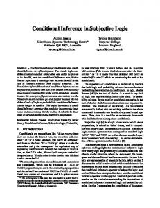
apply (7) (7) apply

Inspection of (21) and (22) and assuring that αk+ > αk for k = 1, . . . , K leads to ∑K 1 + j=1 αj + s ≥ . (30) i li 1 + ∑min K α l j=1

j j

apply (8) (8) apply

Also, s+ should be as close as possible to the values of the s+ k ’s given in (28) so that the Dirichlet approximation to the posterior is no more or less optimistic than it needs to be. Since ¯lk ≥ mini li and lk ≥ mini li , and using (28), it is clear that sk ≤ s+ . (31)

apply (32) (32) apply

Figure 1. Steps for the measurement update in subjective logic where class appearances are partially observed via the measurements.

Therefore, fitting any of the variances of the pk ’s is insufficient to avoid a reduction in at least one of the αk ’s. Therefore, the updated Dirichlet precision should be set to the lower bound in (30) so that subjective logic does not become more confident in the updated beliefs than necessary. Overall, the updated Dirichlet parameters are ( ) αk 1 + ∑K lk α l j=1 j j . αk+ = min 1 + ∑K iαli l j=1

For the first set of examples, the initial uncertainty is set to u = 0.1. Figure 2 plots the updated Dirichlet and opinion scores as a function of lk . In these plots lk ≥ 1, because the lk < 1 case is equivalently explained by transposing the value for α1 and α2 , or equivalently b1 and b2 . Figure 2(a) shows that the incremental update in α2 is bounded by zero and one. Note that (32) indicates that the incremental update in α1 is zero, i.e., ∆α1 = 0, in all cases. When lk = 1, the measurement is vacuous, and the incremental update is always zero. This means that updated subjective logic opinion scores are equivalent to the initial scores. As lk → ∞, the observation becomes visible and the incremental update is one. For a given value of lk , the incremental update becomes larger as the initial value of α2 grows. Note that α1 +α2 = 20 since u = 0.1 and W = 2 (see (8a)). In other words, the measurement strength increases as the Dirichlet parameters demonstrate more bias towards the singleton being espoused by the observation likelihood.

(32)

j j

To perform the measurement update on multinomial opinions, the opinions are transformed to Dirichlet parameters via (7), α is updated via (32), and finally, the updated α+ is mapped back into updated opinions via (8). Figure 1 summarizes these steps for measurement updates within subjective logic. We refer to the difference between the updated and prior Dirichlet precision as the measurement strength ∑K ∑K K ∑ j=1 αj j=1 αj lj − mini li + ξ= (αj − αj ) = . (33) ∑K j=1 αj lj + mini li j=1

Figures 2(b)-(d) show the updated opinion scores as a function of l2 for the first set of examples. Note that the curves in these plots correspond to the curves in Figure 2(a) as the opinion scores and Dirichlet parameters are related via the bijective transformations given in (7) and (8). Comparing Figures 2(a) and (b), it is clear that the incremental update in α2 is inversely related to the updated uncertainty. For the vacuous observation, the uncertainty remains at u = .1. As lk → ∞, the observation becomes completely visible, and given that u = 1 initially and W = 2, then by (16), the uncertainty decreases to a value of u ≈ .0952.

Clearly, 0 ≤ ξ ≤ 1. When the measurement is vacuous, ξ = 0 as none of the Dirichlet parameters are incremented. For the visible observation case, i.e., li = δi−k , then ξ = 1. In fact, as long as any of the class likelihoods is equal to zero, the measurement strength is one.

5. M EASUREMENT U PDATE E XAMPLES The measurement strength given by (33) depends on either how decisive the measurement is in terms of rejecting a class, i.e., the minimum likelihood is near zero, or how the observation likelihood correlates with the opinion score (or equivalently the Dirichlet parameters). This subsection employs examples of binomial opinions to illustrate this. In all examples, the base rate is uniform, i.e., ak = 0.5 for k = 1, 2, and W = 2. Clearly, the updated opinions are invariant to the the overall scaling of the likelihood values (see (32)). Thus for binomial opinions, the likelihood is parameterized by a single value. Here we let l = [1, l2 ]. When l2 = 0 or l2 = ∞, the observation is fully visible where class k = 1 or k = 2 is observed, respectively.

Figures 2(c) and (d) demonstrate that when the observation likelihood is in agreement with beliefs, the beliefs do not change very much, as the decrease in the uncertainty can only change the beliefs by at most a value of 0.048. On the other hand, when the observation likelihood is in disagreement with the initial beliefs, mass is transferred between the two beliefs, and the transferring of the mass becomes more pronounced as either the observation becomes more confident, i.e., lk increases, or as the initial opinion scores provides more mass for b1 than b2 . The next set of examples demonstrate how Dirichlet and opin6

1

1

0.9

0.9

0.8

0.8

0.7

0.7 α1 = 1, α2 = 19 α1 = 5, α2 = 15

0.4 0.3 0.2

0.5

α1 = 10, α2 = 10

0.4

α1 = 15, α2 = 5

0.3

1

2

10

0.1 0 0 10

3

10

u = 1.000 u = 0.500 u = 0.100 u = 0.010

0.2

α1 = 19, α2 = 1

0.1 0 0 10

0.6 2

0.5

∆α

∆ α2

0.6

10

l2

1

b = 0.2, b = 0.7

0.9

0.101

b = 0.5, b = 0.5

0.8

0.1

b1 = 0.7, b2 = 0.2

0.7

b1 = 0.9, b2 = 0.0

0.6

1

2

1

0.099

2

unew

unew

1

b1 = 0.0, b2 = 0.9

0.102

0.5

0.098

0.4

0.097

0.3

0.096

0.2 0.1 1

2

10

10

3

0 0 10

10

l2

1

3

10

(b) 0.5

0.9 0.8

0.4

0.7 0.6 0.5

bnew 1

bnew 1

10 l2

1

0.4

0.3 0.2

0.3 0.2

0.1

0.1 1

2

10

10

3

0 0 10

10

l2

1

2

10

10

3

10

l2

(c)

(c)

1

0.5

0.9 0.8

0.4

0.7 0.6 0.5

bnew 2

bnew 2

2

10

(b)

0.4

0.3 0.2

0.3 0.2

0.1

0.1 0 0 10

3

10

(a)

0.103

0 0 10

10 l2

(a)

0.095 0 10

2

10

1

2

10

10

3

0 0 10

10

l2

1

2

10

10

3

10

l2

(d)

(d)

Figure 2. Updated parameters for various skew in Dirichlet parameters when the likelihood of the observation is l = [1, l2 ] u = 0.1, a = [0.5, 0.5], and W = 2: (a) Incremental update on α2 , (b) updated u, (c) updated b1 , and (d) updated b2 .

Figure 3. Updated parameters for various levels of uncertainty when the likelihood of the observation is l = [1, l2 ] b1 = b2 , a = [0.5, 0.5], and W = 2: (a) Incremental update on α2 , (b) updated u, (c) updated b1 , and (d) updated b2 .

7

ion scores change for various values of uncertainty. In these examples, the belief masses are equal, i.e., b1 = b2 = u/2. Again, these plots demonstrate the transition from a vacuous observation, i.e., l2 = 1, to a completely visible observation, i.e., l2 = ∞. Figure 3(a) demonstrates that for a fixed lk , the incremental update on α2 becomes larger as uncertainty decreases. However, the value of this increment saturates as u goes to zero. Figures 3(b)-(d) simply show that the observations have greater impact when the initial uncertainty is higher. This is simply a fact that the differences between the initial and updated values for visible observations is larger (see (16)).

respectively. For the product rule, the threshold regularization scheme described in [8] was employed to reduce the veto effect exhibited by the product rule. All likelihood values below the threshold τ = 2.22 × 10−16 were set to τ .2 For the subjective logic method, the baseline rates are set to ak = 1/K with W = 2. The class label chosen by subjective logic is the one associated to the largest belief bk , which for the uniform baseline rates, is equivalent to the largest αk . Also, using uniform baseline rates means that the sum rule is equivalent to the na¨ıve subjective logic approach (see (17)). The simulations consider K = 8 for two cases of the class appearance probabilities:

In all these examples, the measurement strength ξ = ∆α2 since ∆α1 = 0 (see (33)). The larger the measurement strength, the larger the drop in uncertainty due the fact that uncertainty is inversely proportional to Dirichlet precision. Since l = [ 1 l2 ] where l2 > 0, the observation likelihood is positively correlated to the current opinion when α2 > α1 or b2 > b1 , and it is negatively correlated when α2 < α1 or b2 < b1 . As can be seen from these examples, the measurement strength is highly dependent on the how the observation likelihood correlates to the current opinion. For instance, positive correlation leads to a larger measurement strength. For stronger opinions, i.e., larger spread between α1 and α2 , or for stronger observations, i.e., larger l2 , the measurement strength increases. Furthermore, the measurement strength also depends on the value of uncertainty for the current belief. For multiple measurement updates, the ordering of the observation likelihoods in updating the beliefs via (32) matters, as some observation likelihoods better correlate with the current opinion than others. Overall, when multiple observations are incorporated, the final updated belief is not invariant to the ordering of how updates are incorporated. We plan to investigate to what extent the belief values can change due to various orderings of the hidden observations in future work.

1. p = [ 1 0 0 0 0 0 0 0 ], and 1 2. p = 18 [ 8 4 1 1 1 1 1 1 ]. For both cases, the ground truth target class is k = 1. The first case represents the traditional classification paradigm when the sensor/target model is known. It is also a special case of the target appearance model. The second case demonstrates classification performance when the target appearance can cause confusion. In some sense, one can view the class appearance model as introducing noise into the likelihood for the traditional classification paradigm. The simulation also considers two cases for the spread of the class data: 1) σ 2 = 0.25, and 2) σ 2 = 1. The first case represents the conditions when the classes are well-separated so that the class likelihood given by (1) will typically exhibit one large element. The second case leads to likelihoods exhibiting more confusion between the classes. Overall, four cases are considered: (a) (b) (c) (d)

p=[ 1 p=[ 1 1 p = 18 [ 1 p = 18 [

0 0 0 0 0 0 0 0 0 0 0 0 0 0 8 4 1 1 1 1 1 8 4 1 1 1 1 1

] and σ 2 = 0.25; ] and σ 2 = 1; 1 ] and σ 2 = 0.25; 1 ] and σ 2 = 1.

For all four cases, the simulations considered the fusion of up to 1000 classifiers, and the results were averaged over 1000 Monte Carlo realizations. While for most practical classifier fusion applications, the number of classifiers will be at most in the order of 10s of classifiers, this analysis provides insights into how the four cases affect classification performance and how many classifiers would be necessary to achieve good performance.

6. S IMULATIONS This section investigates the utility of subjective logic for classifier fusion through simulations. Using the data appearance model for Section 2, there is an underlying pmf describing the probability that a target appears as one of the K classes for an arbitrary sensor modality and viewing direction under random environmental (or operating) conditions. For a given sensor modality, viewing geometry, and class appearance, the sensor data represents a realization of a random process described by a known pdf. For simplicity, the simulations assume that the density function conditioned on the class appearance is the same for all sensor modalities and geometries. Specifically, the simulations generate K × 1 vectors representing the sensor data. Given the k-th target appearance, the sensor data is drawn from a Gaussian distribution with mean ek and covariance σ 2 I, i.e., } { 1 1 f (x|z = k) = √ exp − 2 ∥x − ek ∥2 . (34) 2σ ( 2πσ 2 )K

Figure 4 provides the probability of correct classification Pcc versus the number of fused classifiers for the three fusion method over the four cases. These plots also include onesigma error bars, which are very tight because of the averaging over 1000 Monte Carlo realizations. Clearly, Pcc increases monotonically with the number of classifier observations. As confusion is introduced via the class appearance probability p or the class spread σ 2 , more classifiers are necessary to achieve Pcc near one. The axes in the plots for the four cases are different to reveal when each fusion method reaches close to Pcc = 1 performance. For case (d) this means that the x-axis reveals all 1000 classification observations. The drop from near-perfect classification to zero classification for the product rule around 300 classifier observations is due to the veto property where precision errors catches up to the regularization scheme. This drop phenomena actually occurs in all four cases and would be seen by extending out the x-axis in Figures 4(a)-(c). The

Once the data is generated, the class likelihood is computed via (1) to model the classifier output. Note that in the data space, the distances between the clusters representing the K classes, e.g., Mahalanobis distance between class centroids, are all equal. Then the classifiers are fused via (2), (4), and (32) for the product rule, sum rule, and subjective logic methods,

2τ

8

is the smallest number that can be added to one in double precision.

drop occurs sooner for more noisy measurements (larger σ) or for more confusion (or entropy) in the ground truth appearance probability p. Leaving the veto effect aside, the product rule is significantly better for the first two cases because for the traditional classifier paradigm, the product rule is the likelihood ratio test that is optimal in the NeymanPearson sense [21]. For the last two cases, the sum rule can outperform the product rule. For the cases of tight class cluster, i.e., (a) and (c), subjective logic performs robustly. It is slightly better than the sum rule for case (a), and it is slightly worse than the sum rule and better than the product rule for case (c). For the cases where the class cluster have larger spread, i.e., (b) and (d), the subjective logic method does not perform as well.

Prob. of Correct Classification

1 0.95 0.9 0.85 SL Sum Product

0.8 0.75 0.7

The results in Figure 4 seem to indicate that the sum rule is more robust than subjective logic for classification. It should be noted that subjective logic is designed to track the current belief in singletons (or class labels), and it was not necessarily designed to determine which singleton (or class label) is associated to the largest value of pk .

2

4 6 8 Number of Hidden Observations

10

(a)


1

Figure 5 plots how well the sum rule (equivalently the na¨ıve method in (17)) and subjective logic are able to estimate the underlying appearance probability p by transforming the current values of α to p via (10). The figure provides plots of the Kullback-Liebler divergence along, with one-sigma error bars between the estimated p and the ground truth, for all four cases. The product rule is not considered because it simply attempts to put all the mass in the cumulative likelihood associated to the true class, which makes no sense as a appearance probability estimator. For all four cases, subjective logic is significantly better at estimating p than the sum rule. This difference is more pronounced for the cases associated to larger class spread σ 2 . As the number of classifiers to fuse increases, the subjective logic estimates of p appear to be converging to the ground truth so that the KL divergence goes to zero. On the other hand, the estimated p via the sum rule seems to converge to something other than the ground truth.

0.9 0.8 0.7 SL Sum Product

0.6 0.5 0.4

5

10 15 20 25 30 35 Number of Hidden Observations

40

(b)


1

Figures 6 and 7 illustrate the convergence of the estimated p for subjective logic and the sum rule, respectively, under simulation cases (c) and (d). The bars represent the average ˆ over the 1000 Monte-Carlo estimate of the elements of p realizations as the number of fused classifies goes from 10 to 100 to 1000. These plots also provide one-sigma error bars, and the ‘◦’ markers represent the ground truth. The upper and lower rows in Figures 6 and 7 represent simulation cases (c) and (d), respectively. Since the baseline rate is uniform, i.e., ak = 1/K, the subjective logic method tends to underestimate pk values greater than 1/K and overestimate pk values less than 1/K. Overall, the subjective logic estimate is getting closer to the ground truth, and the error bars are getting tighter as the number of classifiers fused increases. The convergence is much slower for case (d) where σ 2 = 1. On the other hand, the sum rule mean values are holding steady as the the number of fused classifiers increases, and these values are far from the ground truth. However, the error bars are tighter for the sum rule than for subjective logic.

0.9 0.8 0.7 0.6 SL Sum Product

0.5 0.4 0

50 100 Number of Hidden Observations

150

(c)


1

0.8

0.6

0.4

0.2

0 0

Figure 8 plots the cumulative Dirichlet precision as classifier observations are fused. For the case of well separated class clusters, i.e., σ 2 = 0.25 the precision is tracking the number of observations. This means that the observation strengths of all updates are close to one. On the other hand, for the cases of σ 2 = 1, the strength of many of the observation updates are less than one. Interestingly, it is this case when

SL Sum Product

200 400 600 800 Number of Hidden Observations

1000

(d)

Figure 4. Probability of correct classification versus number of fused classifiers when using the product rule, sum rule, and subjective logic over the four cases (a)-(d).

9

SL Sum

KL Divergence

1.5

1

0.5

0.4

0.4

Observation Probability


2

0.5

0.3

0.2

0.1

0

1

2

3

3

1000

SL Sum

2.5

1

2

3

0.5

0.4

0.4

0.3

0.2

0.1

1

2

3

7

8

4 5 6 Object Index

7

7

8

7

8

0.3

0.2

0.1

0

8

1

2

3

(c)

2

4 5 6 Object Index

(b)

0.5

0

4 5 6 Object Index

(d)

0.5

0.5

0.4

0.4

1 0.5 0 0


0.2

0.1

0

0.3

0.2

0.1

1

2

3

4 5 6 Object Index

7

8

0

1

2

(e) SL Sum

0.6

0.3

1000

(b) 0.7


1.5 Observation Probability

KL Divergence

0.1

0

8




(a)

KL Divergence

7

0.2

(a)

0.5

0 0

4 5 6 Object Index

0.3

3

4 5 6 Object Index

(f)

Figure 6. Estimates of p from subjective logic when the ground truth is p = [ 8 4 1 1 1 1 1 1 ]/18 after fusion of Q classifiers: (a) Q = 10, σ 2 = 0.25, (b) Q = 100, σ 2 = 0.25, (c) Q = 1000, σ 2 = 0.25, (d) Q = 10, σ 2 = 1, (e) Q = 100, σ 2 = 1, and (f) Q = 1000, σ 2 = 1.

0.5 0.4 0.3 0.2

the classification power of subjective logic can be inferior to the sum rule. It appears that Dirichlet update in (32) achieves accuracy in representing the belief in the class appearance at the expense of classification accuracy. This update is discounting likelihoods that demonstrate class confusion, which in turns lowers the reduction in the variance. On the other hand, the sum rule ignores this discounting to achieve lower variance at the benefit of better classification. However, by ignoring this discounting and by also ignoring the correlation of the likelihood with current belief, the implementation of the sum rule via the na¨ıve update in (17) is not tracking the belief values.

0.1 0 0


1000

(c) 0.7

SL Sum

KL Divergence

0.6 0.5 0.4 0.3 0.2

7. C ONCLUSIONS

0.1

This paper investigated classifier fusion from the perspective of subjective logic. This perspective considers a new sensor/target model that roughly accounts for the disparity of training and testing data as operating conditions vary. The model consists of an underlying class appearance probability, so that the actual class likelihoods are a mixture of the trained ones. The membership of the target to an actual class is considered to be the class associated with the largest appearance probability. The framework of subjective logic was expanded to accommodate the fact that for a given sensor measurement, the actual class appearance is not observed.

0 0


1000

(d)

Figure 5. Kullback-Liebler distance between expected and actual P versus number of fused classifiers when using the sum rule and subjective logic over the four cases (a)-(d).

10

0.5

0.4

0.4

0.3

0.2

0.1

0

1

2

3

4 5 6 Object Index

7

800

0.3

600 0.1

1

2

3

0.4

0.4

0.3

0.2

0.1

1

2

3

4 5 6 Object Index

7

1000 1

2

3

0.3

0.2

0.1

(e)

4 5 6 Object Index

7

8

800

σ = 0.5 σ = 1.0

7

8

600 Σαi



0.4

4 5 6 Object Index

1000

(d)

0.4

3


(a)

0.1

0

8

0 0

0.2

0.5

2

400

8

200

(c)

1

7

0.3

0.5

0

4 5 6 Object Index

(b) 0.5



(a) 0.5

0

σ = 0.5 σ = 1.0

0.2

0

8

1000

Σαi



0.5

400

0.3

0.2

200 0.1

0

1

2

3

4 5 6 Object Index

7

0 0

8

(f)


1000

(b)

Figure 7. Estimates of p from the na¨ıve subjective logic updates (equivalently the sum rule) when the ground truth is p = [ 8 4 1 1 1 1 1 1 ]/18 after fusion of Q classifiers: (a) Q = 10, σ 2 = 0.25, (b) Q = 100, σ 2 = 0.25, (c) Q = 1000, σ 2 = 0.25, (d) Q = 10, σ 2 = 1, (e) Q = 100, σ 2 = 1, and (f) Q = 1000, σ 2 = 1.

Figure 8. Dirichlet precision as a function of number of fused classifiers: (a) Simulations cases (a)-(b), and (b) simulation cases (c)-(d).

Rather, the measurement leads to a class likelihood. The expanded version of subjective logic uses the class likelihood to update the multinomial opinion by considering the fact that subjective logic maps the multinomial opinion to a Dirichlet distribution for class probabilities. The updated subjective logic framework determines the best Dirichlet fit to the posterior when the sensor measurements lead to class likelihoods (via the classifier) and not direct observations. Simulations demonstrate that when the assumed appearance model is correct, the expanded subjective logic is able to provide good estimates of the appearance probabilities. However, to this end, subjective logic does not necessarily lead to the best means to fuse classifiers. This is likely because subjective logic discounts class likelihoods that demonstrate class confusions. The sum rule for classification fusion is more robust. In essence, subjective logic is designed to be an estimator and not a classifier. Estimation and classification are two difference functions.

Kronecker delta function. Subjective logic can be considered for many applications beyond the fusion of classifiers, and for many of these applications, evidence is not built upon direct observations of singletons. Therefore, future work can investigate the utility of the expanded subjective logic framework for these applications. Finally, the likelihood updates for subjective logic are not associative in the sense the results can differ for various orderings of the likelihoods in the update. Future work will study the extent of how the permutations of the ordering of the updates affect the spread of the final subjective opinions.

Future work can investigate whether or not a classification fusion rule exists that is more robust than the sum rule for the class appearance model. Because the appearance probabilities are not known a priori, a uniformly most powerful (UMP) test does not exist as it cannot be better than the product rule when the appearance model does not include class mixing, i.e., the ground truth appearance probability is a 11

A PPENDICES A. M OMENTS OF THE P OSTERIOR FROM M EASUREMENTS OF H IDDEN O BSERVATIONS

B. C ALCULATION

mk − vk =

Starting with the posterior as given by (20), the first order moments for its marginals pk are = P

pk f (p|α, x)dp,

(35)

∫ ∑K i=1 li αi pk fβ (p|{α + ei })dp, (36) ∑K P j=1 lj αj   ∑K ∫ K ∑ li pi pk  αj  ∑i=1 fβ (p|α)dp, (37) K P j=1 lj αj j=1 ∑K l α (α + δ ) (∑ i=1 i )i ( k ∑i−k ), (38) K K l α 1 + α j j j j=1 j=1

=

=

=

=

j=1

∫

mk − vk

= =

(39)

fβ (p|{α + ei }),

=

(41) =

2 i=1 li αi pk

=

=

(∑

∑K

j=1 lj αj

fβ (p|α + ei )dp,

(44)

∑K

+ 1)(αk + δi−k ) i (α + δ i=1 li α ) ( k ∑i−k )( ), ∑ K K 1 + j=1 αj 2+ K j=1 lj αj j=1 αj

)

( αk +

αk lk ρ 2

(s + 1)

)2 , (53) (54)

αk (s + 2) αk lk2

, (s + 1)2 (s + 2) αk ρ (ρ − αk lk + (s − αk ) (ρ + lk )) ρ2

(55)

ρ2 (s + 1)2 (s + 2) αk (s + 2) (ρlk − αk lk2 )

, ρ2 (s + 1)2 (s + 2) ( ( ) ) αk α ¯k ρ ¯ lk + ρ + lk + (s + 2) ¯ lk lk ρ2 (s + 1)2 (s + 2)

.

(56)

Thus, the Dirichlet precision to match the variance associated to pk is ( ) ρ (s + 1) ¯lk + ρ + lk + ) ), sk = ( (¯ (57) ρ lk + ρ + lk + (s + 2) ¯lk lk s+1 = (58) , ¯ lk lk 1 + ρ(s+2) ¯ (lk +ρ+lk ) s+1 = . (59) (s+2) 1 + ρ (1+α¯ )l−1 ¯−1 ( k k +(1+αk )lk )

∑K

P

=

(43)

2αk lk ρ

ρ2 (s + 1)2 (s + 2)

+ =

=

(49)

− (s + 1) (s + 2) ( 2 ) αk (s − αk + 1) ρ + 2ρlk

−

∫ ∫

lj αj .

( (αk + 1) αk +

Likewise, the non-central second order moments for its marginals pk are p2k f (p|α, x)dp,

K ∑

Similarly, the denominator of (26) is

=

P

, (48)

(s + 1) (s + 2)

αk ((s − αk + 1) (ρ + lk ) − (αk + 1)lk ) , (50) ρ (s + 1) (s + 2) αk ((ρ − αk lk ) + (s − αk ) (ρ + lk )) , (51) ρ (s + 1) (s + 2) ( ) αα ¯ k ¯ lk + ρ + lk , (52) ρ (s + 1) (s + 2)

respectively.

=

)

where α ¯ k and ¯lk as defined in (29) represent the total Dirichlet precision and average likelihood, respectively, associated to the complement of the k-th singleton in the frame.

αi (αk + δi−k ) ) , (42) )( pi pk fβ (p|α)dp = (∑ ∑K K P 1 + j=1 αj j=1 αj

vk

−

2αk lk ρ

The numerator can be simplified to

vk − m2k

αj

(s + 1)

( (αk + 1) αk +

j=1

for k = 1, . . . , K. Note the jumps from (36) to (37) and from (37) to (38) are due to the following identities [20], pi fβ (p|α) = ∑K

α k lk ρ

ρ=

(40)

ai

αk +

=

αk + ∑Kαk llk α j=1 j j ( ), ∑K 1 + j=1 αj

P RECISION

where s is the Dirichlet precision given by (12) and ρ is the correlation between the prior Dirichlet parameters and the observation likelihoods

∫ mk

OF THE

The numerator of (26) is

(45)

(∑ ) K (1 + αk )αk i=1 li αi (∑ )( )( ) (46) ∑ ∑ K 1+ K 2+ K j=1 lj αj j=1 αj j=1 αj ∑K i−k + 1) i=1)li(αi δi−k (2αk +)δ( ), + (∑ ∑K ∑ K l α 1 + α 2+ K j=1 j j j=1 j j=1 αj ) ( 2αk lk (1 + αk ) αk + ∑K j=1 lj αj ( )( ), (47) ∑ ∑K 1+ K α 2 + j=1 j j=1 αj

Substitution of (12) and (49) into (59) leads to (28).

R EFERENCES [1]

for k = 1, . . . , K. 12

J. Kittler, M. Hatef, R. P. Duin, and J. Matas, “On combining classifiers,” IEEE Trans. on Pattern Analysis

[2]

[3]

[4]

[5]

[6]

[7]

[8] [9]

[10]

[11]

[12]

[13]

[14]

[15]

[16] [17] [18]

and Machine Intelligence, vol. 20, no. 3, pp. 226–239, Mar. 1998. D. Ruta and B. Gabrys, “An overview of classifier fusion methods,” Computing and Information Systems, vol. 7, no. 1, pp. 1–10, Feb. 2000. L. I. Kuncheva, “Theoretical study on six classifier fusion strategies,” IEEE Trans. on Pattern Analysis and Machine Intelligence, vol. 24, no. 2, pp. 281–286, Feb. 2002. S. A. Rizvi and N. M. Nasrabadi, “Fusion of FLIR automated target recognition algorithms,” Information Fusion, vol. 4, no. 4, pp. 247–258, Dec. 2003. T. D. Ross, M. Doug R, E. P. Blasch, K. J. Erickson, and B. D. Kahler, “Survey of approaches and experiments in decision-level fusion of automatic target recognition (ATR) products,” in Proc. of the SPIE, vol. 6567, Apr. 2007. D. M. Tax, M. van Breukelen, R. P. Duin, and J. Kittler, “Combining multiple classifiers by averaging or by multiplying?” Pattern Recognition, pp. 1475–1485, 2000. F. M. Alkoot and J. Kittler, “Improving the performance of the product fusion strategy,” in Proc. of the 15th International Conference on Patter Recognition, vol. 2, Barcelona, 2000, pp. 164–167. ——, “Modified product fusion,” Pattern Recognition Letters, vol. 23, pp. 957–965, 2002. V. Cevher, F. Guo, A. C. Sankaranarayanan, and R. Chellappa, “Joint acoustic-video fingerprinting of vehicles, part ii,” in Proc. of the IEEE International Conference on Acoustics, Speech, and Signal Processing (ICASSP), 2007. V. Cevher, R. Chellappa, and J. H. McClellan, “Joint acoustic-video fingerprinting of vehicles, part i,” in Proc. of the IEEE International Conference on Acoustics, Speech, and Signal Processing (ICASSP), 2007. C. Bisdikian, L. M. Kaplan, M. B. Srivastava, D. J. Thornley, D. Verma, and R. I. Young, “Building principles for a quality of information specification for sensor information,” in Proc. of the International Conference on Information Fusion, Seattle, WA, Jul. 2009. E. R. Keydel, S. W. Lee, and J. T. Moore, “MSTAR extended operating conditions: a tutorial,” in Proc. of the SPIE, vol. 2757, 1996. G. Healey and D. Slater, “Models and methods for automated material identification in hyperspectral imagery acquired under unknown illumination and atmospheric conditions,” IEEE Trans. on Geoscience and Remote Sensing, vol. 37, no. 6, pp. 2706–2717, Nov. 1999. J. A. Ratches, “Review of current aided/automatic target acquisition technology for military target acquisition tasks,” Optical Engieering, vol. 50, no. 7, Jul. 2011. A. Jøsang, S. Marsh, and S. Pope, “Exploring different types of trust propogation,” in Proc. of the 4th International Conference on Trust Management (iTrust), Pisa, Italy, May 2006. A. Jøsang, “Subjective logic,” Jul. 2011, draft book in preparation. G. Shafer, A Mathematical Theory of Evidence. Priceton University Press, 1976. K. Fukunaga, Introduction to Statistical Pattern Recognition. Academic Press, Inc., 1990.

[19] A. Jøsang and D. McAnally, “Multiplication and comultiplication of beliefs,” International Journal of Approximate Reasoning, vol. 38, no. 1, pp. 19–51, 2004. [20] A. Gelman, J. B. Carlin, H. S. Stern, and D. B. Rubin, Bayesian Data Analysis. Boca Raton, FL: Chapman & Hall/CRC, 1995. [21] T. K. Moon and W. C. Stirling, Mathematical Methods and Algorithms for Signal Processing. Upper Saddle River, NJ: Prentice Hall, 2000.

Lance M. Kaplan (SM’00) received the B.S. degree with distinction from Duke University, Durham, NC, in 1989 and the M.S. and Ph.D. degrees from the University of Southern California, Los Angeles, in 1991 and 1994, respectively, all in Electrical Engineering. From 1987-1990, Dr. Kaplan worked as a Technical Assistant at the Georgia Tech Research Institute. He held a National Science Foundation Graduate Fellowship and a USC Dean’s Merit Fellowship from 1990-1993, and worked as a Research Assistant in the Signal and Image Processing Institute at the University of Southern California from 1993-1994. Then, he worked on staff in the Reconnaissance Systems Department of the Hughes Aircraft Company from 1994-1996. From 1996-2004, he was a member of the faculty in the Department of Engineering and a senior investigator in the Center of Theoretical Studies of Physical Systems (CTSPS) at Clark Atlanta University (CAU), Atlanta, GA. Currently, he is a researcher in the Networked Sensing and Fusion branch of the U.S. Army Research Laboratory. Dr. Kaplan serves as Associate Editor-In-Chief and EO/IR Systems Editor for the IEEE Transactions on Aerospace and Electronic Systems (AES). In addition, he is the tutorials editor for the IEEE AES Magazine, and he also serves on the Board of Governors of the IEEE AES Society. He is a three time recipient of the Clark Atlanta University Electrical Engineering Instructional Excellence Award from 1999-2001. His current research interests include signal and image processing, automatic target recognition, information/data fusion, and resource management.

Supriyo Chakraborty (StM’10) received the B.Tech. degree in computer science and engineering from National Institute of Technology (NIT), Warangal, India, in 2001, the M.Tech. degree in electrical engineering from Indian Institute of Technology (IIT), Bombay, India, in 2006 and is currently pursuing the Ph.D. degree in electrical engineering at the University of California, Los Angeles. He has worked as a software engineer at HCL Technologies from 2001 to 2003 and at Cisco Systems from 2006 to 2008. He is the recipient of the Qualcomm Innovation Fellowship award for the year 2010-2011. His research interests are in network measurements, sensor networks, information privacy and security. 13

Chatschik Bisdikian (F’04) is a Research Staff Member with the Network Management Department at IBM T. J. Watson Research Center. He has been with IBM Research since 1989 and has worked in numerous projects covering a variety of research topics in communications, networking, pervasive computing, IPTV services, computer system management, quality of information for sensor networks, and so on. He has authored over 120 peerreviewed papers, holds several patents in the aforementioned areas, and co-authored the book Bluetooth Revealed (Prentice Hall). He has served as the Editor-in-Chief of IEEE Network Magazine, where he currently serves as the Senior Technical Editor. He also serves in the editorial board of the Pervasive and Mobile Computing journal and had served in the editorial boards of IEEE Journal on Selected Areas in Communications and Telecommunication Systems journal; he has also guest edited several special issues on various topics. He served as the Technical Program Chair for IEEE PerCom’09, and served as Chair for the IEEE Int’l Workshop on Information Quality and Quality of Service (IQ2S’10 and ’11) and the IEEE Workshop on Quality of Information for Sensor Networks (QoISN’08). He received the 2002 best tutorial award from IEEE Communications Society for his paper titled ”An Overview of the Bluetooth Wireless Technology” and the 2010 IEEE RTSS best paper award for his paper titled ”Quality Tradeoffs in Object Tracking with Duty-cycled Sensor Networks.” He is an IEEE Fellow and a member of the Academy of Distinguished Engineers and Hall of Fame of the School of Engineering of the University of Connecticut.

14