Fusion of Multi-Frequency Eddy Current Signals by Using Wavelet Analysis Method Zheng, Liu Institute for Aerospace Research National Research Council Canada Montreal Road 1191, M-14, Room 206 Ottawa ON, K1A 0R6, Canada
[email protected]
Lingqi Li, Kazuhiko Tsukada and Koichi Hanasaki Earth Resources Engineering Department Graduate School of Engineering, Kyoto University Kyoto, Japan.
[email protected]
presents some limitations in term of defect detection and characterization. The use of more than one NDT system or signal is usually required for accurate flaw detection and/or qualification. This is the concept of data fusion. Although the concept of multisensor data fusion and integration has been applied to military applications for several years, only recently did the the NDT community realise that it could be of benifit to the field of nondestructive evaluation (NDE). As reported in the literature, some researchers have shown great enthusiasm for this topic [3,8,9].
Abstract - This paper presents a novel scheme to fuse one-dimensional multi-frequency eddy current signals by using multiresolution discrete wavelet analysis method. This technique consists of three steps. First, raw signals are preprocessed and decomposed into approximations and details at different resolution levels. The discrete wavelet transform is adopted at this stage. Then, several fusion processes are implemented in the coefficients domain. Finally, the inverse discrete wavelet transform is achieved to get the fusion result. In this technique, we develop a new mask-signal-modulated fusion algorithm to fuse in coefficients domain. It is performed and compared with other fusion methods based on the criteria of signalto-noise ratio of the fused result. From our experiments, it demonstrates a better performance and shows a promising application on the two-dimensional multifrequency eddy current signals.
In this paper, we present a novel fusion algorithm to fuse one-dimensional MFECT signals by using multiresolution discrete wavelet analysis method. Wavelet transform is a relatively new signal processing technique [4]. The multiresolution analysis scheme underlying wavelet transform allows us to extract simultaneously the frequency and spatial information to get the local characteristics of signals. These coefficients stand for the features of signals and can be fused to enhance the signalto-noise ratio (SNR). In addition, a fast implementation of the discrete wavelet transform (DWT) makes possible the real-time processing of the MFECT signals.
Keywords: Nondestructive testing, multi-frequency eddy current testing, data fusion, wavelet analysis, signal processing.
1
Introduction
Eddy current testing (ECT) is one of the most effective nondestructive testing (NDT) techniques to detect the flaws in conductive materials [1]. It has found its applications to bar, to tube, and to wire testing. Flaws in the tested materials result in a measurable change of the coil (ECT probe) impedance. In ECT, the depth of eddy current is determined by the exciting frequency in such a way that the lower frequency penetrates deeper than the higher one does. It is the so-called skin-effect. In the case the defects exist in both surface and inner specimen, the multi-frequency ECT (MFECT) method is usually adopted [2]. The MFECT signals, however, are usually corrupted by noise and a large number of nondefect signals, including conductivity, permeability, geometry and probe lift-off etc. On the other side, single ECT signal picked up at different frequency carrys limited information and is not enough to reveal the whole characters of the test materials. Indeed, no single NDT method or signal can fully assess the structrual integrity of a mterial. Each method or signal
ISIF © 2002
The rest of this paper is organized as follows. Section 2 briefly reviews the discrete wavelet transform (DWT). The data fusion algorithm based on DWT is presented in section 3. Experimental results and discussion can be found in section 4. Finally, a conclusion is summarized in section 5.
2
Multi-resolution Analysis: Discrete Wavelet Transform
Discrete wavelet transform acts as a popular multiresolution analysis method and plays an important role for signal/image processing [5, 6]. DWT analyzes signal at different frequency bands with different resolutions by decomposing the signal into a coarse approximation and detail information. It employs two sets of functions, called scaling functionsφ(x) and wavelet functionsψ(x), which are associated with the ‘approximation’ and ‘detail’ parts,
108
Take a reference level J in formula (5). There are two sorts of details. Those associated with indices j ≤ J correspond to the scales between 2 j ≤ 2 J which are the fine details. The others, which correspond to j>J, are the coarser details. We group these latter details into
respectively. The DWT of a signal f(x) is defined as the projection of the signal on the set of the wavelet functions ψ j,k (x)
Dwtf ( j , k ) = ∫ f ( x)ψ j , k ( x ) dx
(1)
AJ = ∑ D j
where { ψ j,k(x)} are generated from the same template function ψ (x), called the mother wavelet, using the following formula:
ψ j , k ( x) = 2- jψ (2- j x - k ) .
which defines the approximation of the signal. Then the signal can be summed as
(2)
f ( x ) = AJ + ∑ D j .
+∞
∑
From this formula, it is obvious that the approximations are related to one another by:
A j −1 = AJ + DJ
3
(11)
Fusion in DWT coefficients domain
As summarized in Fig.1, the signal processing approach consists of three steps.
2j
∑ Dwtf ( j, k )ψ j ,k ( x) .
(10)
j≤ J
The DWT coefficients { Dwtf(j,k) } reflect the local characteristics of f(x) both in frequency and space, depending on the scaling parameter j and the shift parameter k. The large coefficients correspond the features of signal, while the small ones represent mostly the noise in the data. The signal can be reciprocally reconstructed from these coefficients through the inverse DWT (IDWT) if the ψ (x) is chosen appropriately
f ( x) =
(9)
j>J
(3)
j =−∞ k =1
3.1 Let us fix j and sum on k. A detail Dj is nothing more than the function
D j ( x) = ∑ Dwtf ( j, k )ψ j ,k ( x) .
To facilitate the DWT implementation, a number of preprocessing steps were performed to remove the sparse spikes from the probe signals, to normalize their magnitudes in a proper way and to align the data for fusion.
(4)
k ∈Z
Let’s look inside of these coefficients. If we sum on j, the signal is the sum of all the details: f ( x) = ∑ D j
Data Pre-processing
ECT @ Frequency 1
(5)
ECT @ Frequency 2
Mask Signal
Data Pre-Processing (Data Alignment)
j∈Z
Discrete Wavelet Decomposition
φ ( x) , the j approximation of signal at the resolution 2 can be
Associated with the scaling function
Feature Set 1
Feature Set 2
Modulating Set
defined as Fusion Implementation
2j
Aj f ( x) = ∑ Af ( j, k )φ j ,k ( x)
(6)
k =1
New Feature Set
where
Inverse DWT
Af ( j , k ) = ∫ f ( x )φ j , k ( j , k ) dx
(7) Fused Signal
and
φ j ,k ( x) = 2− j φ (2− j x − k ) .
Figure 1. Procedure of data fusion
(8)
109
3.2
where 1 ≤
Features fusion in DWT domain
Two MFECT signals, which had been normalized and aligned, were then decomposed into L scale levels using the fast wavelet transform (FWT) algorithm [7]. From equation (10), we have
Mask-signal-modulated combination We also selected one more ECT signal picked up at different excited frequency as the mask signal M. Its DWT coefficients were used to modulate two feature sets of f1 and f2. It was depicted as the dotted section in Fig. 1 and described in Eq. (16).
L
f ( x) = AL ( x) + ∑ Dj ( x) j =1
2L
L
2j
k =1
j =1 k =1
(12)
= ∑ AL (L, k )φL,k ( x) + ∑∑ Dwtf ( j, k )ψ j ,k ( x)
A L ( L , k ) f = A L ( L , k ) f m × A L ( L , k ) f1 + (1 − A L ( L , k ) f m ) × A L ( L , k ) f 2 D w t ( j, k ) f = D w t ( j, k ) f × D w t ( j, k ) f + m 1 (1 − D w t ( j , k ) f m ) × D w t ( j , k ) f 2 (16)
With the level L and wavelet selected appropriately, the DWT coefficients sets, AL ( L, k ) and { Dwtf ( j , k ) }, extracted the salient features at different scales. Therefore, the characters of both the inner and outer defects in material were preserved and transformed into DWT domain. Let the two MFECT signals be f1 and f2. And f denotes the fused signal. Four fusion approaches were applied to these coefficients.
where 1 ≤
3.3 Maximum amplitude selection
j ≤ L , and 1 ≤ k ≤ 2 j .
Signal reconstruction
Based on Eq. (3), inverse discrete wavelet transform was performed to reconstruct the fusion result from the new feature set { AL(L,k)f, {Dwt(j,k)f} }. As presented in the our 1-D MFECT experiment, the SNR of the fused signal was enhanced to make possible of accurate flaw detection and/or characterization.
A L ( L, k ) f = max{ A L ( L, k ) f1 , A L ( L, k ) f 2 } Dwt ( j, k ) f = max{Dwt ( j, k ) f1 , Dwt ( j , k ) f 2 } (13) where 1 ≤
j ≤ L , and 1 ≤ k ≤ 2 j .
j ≤ L , and 1 ≤ k ≤ 2 j .
4
Averaging
Experimental results and discussion
4.1
Specimen and experiment set-up
A L ( L , k ) f = [ A L ( L , k ) f1 + A L ( L , k ) f 2 ] / 2 Dwt ( j , k ) f = [ Dwt ( j , k ) f1 + Dwt ( j , k ) f 2 ] / 2 (14) where 1 ≤
j ≤ L , and 1 ≤ k ≤ 2 j .
(a)
Weighted averaging ECT Coil
Weighted averaging can be used when there is more knowledge towards one NDT technique or signal [2]. Eq. (14) was used to compute weighted-averaging feature set.
(b) X-Y Controller
ECT Impedance Analyzer
w1 × A L ( L , k ) f1 + w2 × A L ( L , k ) f 2 A L ( L, k ) f = w1 + w2 w × Dwt ( j , k ) f1 + w2 × Dwt ( j , k ) f 2 Dwt ( j , k ) f = 1 w1 + w2
RS232C GPIB
(c)
Figure 2. Schematics of specimen and MFECT set-up Two different kinds of ferrous specimen were prepared with simulated cracks both on surface and in inner material, as depicted in Fig. 2 (a) and (b). Figure 2 (c) shows the schematic of MFECT experimental setup. The ECT probe is driven by a X-Y controller to scan the
(15)
110
specimen. The ECT signals are picked up and transfered to impedance-measureing device, which is linked with computer via GPIB.
4.2
1 0.8 0.6 0.4 0.2
MFECT data and fusion results
1 0.8 0.6 0.4 0.2 0
The 1-D MFECT signals from two simulated specimen were processed by using our fusion algorithm addressed in section 3.2. The mother wavelet functions used in the following examples were those proposed by Daubechies [7]. Hereafter, the Daubechies wavelet of the order N was denoted as “DBN”. And the decomposing level was assigned to be 5.
1 0.8 0.6 0.4 0.2 0
E C T@ 100k H z E C T@ 20k H z
To eliminate the influence of the low-frequency probe lift-off noise, DB10 was adopted first to decompose the signals. Due to the high regularity of DB10, this liftoff noise was approximated by the approximation at level 5, A5, and thus was removed by filtering out the A5. Then, the reconstructed signals based on IDWT were again decomposed into 5 fequency levels with the wavelet DB3. The feature sets were achieved effectively because of the good space-frequency-localization characteristic of DB3.
100
200
300
400
500
600 ( b )
100
200
300
400
500
600 ( c )
100
200
300
400
500
600 ( d )
100
200
300
400
500
600
Figure 4. Fusion results of specimen (I) from : (a) maximum amplitude selection, (b) averaging, (c) weighted averaging, and (d) mask-signalmodulated combination.
From the Fig. 3, the defect on the probe-side surface was detected clearly, while the one in inner specimen was not obvious. It was due to the MFECT skin-effect. The fusion results and the SNR of each fusion approach were given in Fig. 4 and Table 1, respectively.
1 0.8 0.6 0.4 0.2 0 100
200
1 0.8 0.6 0.4 0.2 0
300 (a)
400
500
600
1 0.8
E C T@ 20 k H z E C T@ 10 0k H z F us ed s ignal
0.6
100 M as k
1 0.8 0.6 0.4 0.2 0
( a )
200
1 0.8 0.6 0.4 0.2 0
300 (b)
400
500
600 0.4
0.2
100
200
300 (c )
400
500
600
0
Figure 3. Raw ECT signals of specimen (I) and mask signal : (a) raw signal picked up at 20kHz, (b) picked up at 100kHz, and (c) the mask signal.
∑| x∈ N
f ( x ) |2
∑|
f ( x ) |2
200
300
400
500
600
Figure 5. Fused signal of specimen [I] by using the mask-signalmodulated combination method versus the raw signals.
The signals shown in Fig. 3(a) and (b) are the impedance data of the first specimen on exciting frequency 20kHz and 100kHz, respecttively. Fig. 3(c) is the mask signal, which was picked up at 500Hz exciting frequncy. For the location of the simulated cracks (slots) is available, the noise region N and signal regin S can be seperated conveniently. The SNR was defined as the formula (17).
SNR =
100
As depicted in Fig. 4, the fused signals baed on maximum amplitude selection and averaging rules enhanced the inner defect infermation to some extent. But the SNRs were not improved. The SNR from the weighted averaging approach was better than the former two. It is, however, difficult to asign the weights accurately when more knowledges of signals to be fused are not available. In the case the weights are not selectedd carefully, incorrect or conflicting result will be generated and. In the fourth method, we adopted a mask signal which was actually the same ECT signal of the speciman except that it was picked up at a different exciting frequency. The uniform interlink between the mask signal and the ones to
(17)
x∈ S
111
E C T@ 100 k H z
be fused makes the result more realiable. After modulating the DWT coefficients of MFECT signals by the mask feauture set, the inner flaw information was highlight more obviously than the other three method. The SNR was also enhaced more effectively. It can be shown in Fig. 5 and Table 1.
0.6
150
200
0.2 50
100
150
200
1 0.8 0.6 0.2 100
150
200
150
200
100
150
200
0.8 0.6 0.4 0.2
250
(b )
0.8 0.6
250 ( d )
50
0.4
250 ( c )
50
0.4
50
100
0.8 0.6 0.4 0.2
250
(a )
250 ( b )
50
0.4
1 M as k
100
0.8 0.6 0.4 0.2
0.8
0
( a )
50
1
0 E C T@ 200 k H z
1 0.8 0.6 0.4 0.2
100
150
200
250
0.2 0 50
100
150
200
Figure 7. Fusion results of specimen (II) from : (a) maximum amplitude selection, (b) averaging, (c) weighted averaging, and (d) mask-signalmodulated combination.
250
(c )
Figure 6. Raw ECT signals of specimen (II) and mask signal : (a) raw signal picked up at 20kHz, (b) picked up at 100kHz, and (c) the mask signal.
1 E C T@ 1 0 0 k H z E C T@ 2 0 0 k H z F u s e d s ig n a l
0.8
The signals of the specimen (II) were also precessed by using our fusion algorithm. Comparing the raw signals with the result signal, the inner flaw information, which was lost or obscure to be detected, was highlighted effectively even though its SNR was not improved notably. Figs. 7 and 8 and Table 2 give the fusion results.
0.6
0.4
0.2
0 50
100
150
200
250
Figure 8. Fused signal of specimen [II] by using the mask-signalmodulated combination method versus the raw signals.
Table 1. Evaluation of fusion results by SNR (specimen [I]) ECT ECT Maximum @ @ amplitude 20kHz 100kHz selection SNR
6.2183
1.3973
1.5069
Table 2. Evaluation of fusion results by SNR (specimen [II]) ECT ECT Maximum @ @ amplitude 100kHz 200kHz selection SNR
2.0660
2.1322
2.2191
112
Averaging
Weighted Averaging
Mask-signalmodulated combination
2.3740
4.0634
14.5386
Averaging
Weighted Averaging
Mask-signalmodulated combination
2.5562
2.7764
3.4456
5
Conclusion
A novel data fusion approach was discussed to multifrequency eddy current flaw detection based on discrete wavelet transform. Both the signal-to-noise ratio and inner flaw interpretation were enhaced. The effectiveness can be comformed by our one-dimensional MFECT signals fusion results from two kinds of test pieces. The experiment also shows that our fusion algotithm can be applied to the twodimensional MFECT signals. And because the approach can be implemented effeiciently by using the fast wavelet transform, this technique provides a promising method for real-time processing of the MFECT siganls.
References [1] Don E. Bray and Roderic K. Stanley, Nondestructive Evaluation, McGraw-Hill, USA, 1989. [2] P. E. Mix, Introduction to Nondestructive Testing: A Training Guide, John Wiley & Sons, Inc, Canada, 1987. [3] Xavier E. Gros, Application of NDT data fusion, Kluwer Academic Publishers, USA, 2001. [4] Lingqi Li, K.Tsukada and K. Hanasaki, A novel signal processing approach to eddy current flaw detection based on wavelet analysis, Condition Monitoring And Diagnostic Engineering Management, Manchester, UK, 2001, Proc. of the 14 international congress, pp. 153-160. [5] Anthony Teolis, Computational Signal Processing with Wavelet, Birkhäuser, USA, 1998. [6] S.G. Mallat, A theory for multiresolution signal decomposition: The wavelet representation, IEEE Transaction on Pattern Analysis and Intelligence Vol 11, No. 7, pp.674-693, 1989. [7] I. Daubechies, Ten Lectures on Wavelets, CBMSNSF Series in Applied Mathematics, 1992. [8] Liu Z., Tsukada K., Hanasaki K. and Kurisu, M. Two-dimensional eddy current signal enhancement via multifrequency data fusion, Research in Nondestructive Evaluation, Vol 11, No. 3, pp.165-177, 1999. [9] D. Horn and W.R. Mayo, NDE reliability gains from combining eddy-current and ultrasonic testing, NDT & E International, Vol. 33, No. 6, pp.351-362, 2000.
113