Fusion of multi-level decision systems using the Transferable Belief Model David Mercier
Genevi`eve Cron
Universit´e de Technologie de Compi`egne / SOLYSTIC UMR CNRS 6599 Heudiasyc, BP20529 F-60205 Compi`egne Cedex, France Email:
[email protected] [email protected]
SOLYSTIC 14 avenue Raspail F-94257 Gentilly Cedex, France Email:
[email protected]
Thierry Denœux
Myl`ene Masson
Universit´e de Technologie de Compi`egne UMR CNRS 6599 Heudiasyc, BP20529 F-60205 Compi`egne Cedex, France Email:
[email protected]
Universit´e de Picardie Jules Verne UMR CNRS 6599 Heudiasyc, BP20529 F-60205 Compi`egne Cedex, France Email:
[email protected]
Abstract— In this paper, we are interested in the fusion of classifiers providing decisions which are organized in a hierarchy, i.e., for each pattern to classify, each classifier has the possibility to choose a class, a set of classes, or a reject option. We present a method to combine these decisions based on the Transferable Belief Model (TBM), an interpretation of the Dempster-Shafer theory of evidence. The TBM is shown to provide a powerful and flexible framework, well suited to this problem. Special emphasis is put on the construction of basic belief assignments, an important issue which has not yet been fully explored in the literature. We propose an approach extending a former proposal made by Xu, Krzyzak and Suen (1992) in a simpler context. A rational decision modelling allowing different levels of decision is also presented. Finally, the proposed combination is compared experimentally to several simpler alternatives. Index Terms— Decision Fusion, multi-level decisions, belief functions, Dempster-Shafer theory, Evidence theory, classification.
I. I NTRODUCTION Building highly reliable classifiers is an important objective in pattern recognition. An interesting way to achieve this goal consists in the combination of already existing classifiers. Indeed, experimental results ([1], [2]) show that methods based on multiple classifiers generally outperform each individual classifier. As explained by Xu, Krzyzak and Suen in [3], the combination of multiple classifiers includes several problems: selecting the classifiers to combine (types, algorithms, number, . . . ), choosing an architecture for the combination (parallel, cascade, mixtures of both, . . . ), and combining the classifier outputs in order to achieve better performance than each classifier individually. In this paper1 , we focus on the problem of combining clas1 This work is the result of a cooperation agreement between the Heudiasyc laboratory at the Universit´e de Technologie de Compi`egne and the SOLYSTIC company.
0-7803-9286-8/05/$20.00 © 2005 IEEE
sifiers providing decisions which are organized as a hierarchy: decisions can be expressed at different levels. For each pattern to classify, each classifier has the possibility to choose either a class, or a set of classes, or rejection. We assume that the decisions are not associated with any scoring vector, or posterior probabilities. It is a common situation in real world applications. Classifiers providing only class labels are called abstract level classifiers or classifiers of Type 1 in [3]. To combine such classifiers, various combination techniques were proposed such as voting-based systems [3], [4], [5], plurality [6], Bayesian theory [3], Dempster-Shafer theory [3], [7] or classifier local accuracy [8]. Inspired by a former proposal by Xu, Krzyzak and Suen (1992) [3], a combination of these decisions based on the Transferable Belief Model (TBM) ([9], [10]) is proposed. Like all Dempster-Shafer approaches, the assignment of masses is an important task which often determines the success of the combination. Therefore, different assignments are discussed. A decision process allowing different levels of decision is also presented. This paper is organized as follows. The key points of the TBM, an interpretation of the Dempster-Shafer theory of evidence [11] well suited to information fusion, are recalled in Section II. In Section III, we come back to an existing method for combining belief functions in the case of non hierarchical decisions. Then, in Section IV, a model based on the TBM is presented for the combination of multi-level decisions. Finally, Section V describes experimental results and compares the proposed combination with voting-based schemes.
II. T HE T RANSFERABLE B ELIEF M ODEL (TBM): FOUNDATIONS
A. Information representation Let X be a variable taking values in a finite set Ω, called the frame of discernment (or frame). Ω is composed of mutually exclusive elements ω1 , . . . , ωK called atoms. The knowledge held by a rational agent Y , regarding the actual value ω0 taken by X, can be quantified by a belief function defined from the power set 2Ω to [0, 1]. Belief functions can be expressed in several forms: the basic belief assignment (BBA) m, the credibility function bel and the plausibility function pl, which are in one-to-one correspondance. We recall that m(A) quantifies the part of belief that is restricted to the proposition ω0 ∈ A ⊆ Ω and satisfies: X m(A) = 1. (1) A⊆Ω
Thus, a BBA can support a set A ⊆ Ω without supporting any subproposition of A, which allows to account for partial knowledge. Some particular belief functions often used, are defined as follows: Definition 1: The vacuous belief function quantifies total ignorance: mΩ (Ω) = 1. Bayesian belief functions quantify perfect knowledge on X’s value: mΩ (A) 6= 0 ⇒ |A| = 1. B. Handling the knowledge Two distinct pieces of evidence, quantified by BBAs m1 and m2 , may be combined, using a suitable operator. The most common are the conjunctive rule of combination (CRC) and the disjunctive rule of combination (DRC), defined, respectively, as: X m1 ° m1 (B) m2 (C), ∀A ⊆ Ω; ∩ m2 (A) = B∩C=A
m1 ° ∪ m2 (A) =
X
m1 (B) m2 (C), ∀A ⊆ Ω.
B∪C=A
If the two distinct pieces of evidence are trustful enough, the CRC is used. Otherwise, if at least one piece of evidence is reliable, the DRC can be used. C. Decision making When an agent has to select an optimal action among an exhaustive set of actions, rationality principles [12], [13] justify the strategy that consists in choosing the one that minimizes the expected risk (or expected cost). This principle leads to the use of a probability measure P Ω : 2Ω → [0; 1] and a cost function c : A × Ω → IR, where A is the set of possible actions. The optimal action is then the one that minimizes the expected cost (risk) defined by: X ρ(α) = c(α, ω)P Ω ({ω}). (2) ω∈Ω
Therefore, when a decision has to be made, the BBA obtained after the combination must be transformed into a probability measure. One solution proposed in [14] consists in using the pignistic transformation [15], [16] to compute the pignistic probability: X m(A) . (3) BetP ({ω}) = | A | (1 − m(∅)) {A⊆Ω,ω∈A}
Most of the time, classification algorithms do not directly compute a BBA. Thus, to apply the TBM or any model based on the Dempster-Shafer theory, each classifier’s output has to be converted in the form of a BBA. This task is very important as each BBA is supposed to represent all the knowledge provided by a classifier. In particular, BBAs should reflect each classifier’s strenghs and weaknesses. The following section aims at representing the information produced by each classifier through the best possible BBA. III. M ASS ASSIGNMENT THROUGH THE TBM In this paper, decisions are assumed to be the only pieces of information available on each individual classifier. In particular, we will not use the feature vector of pattern x used in others approaches [7], [17]. The BBAs representing the knowledge on each classifier can be built from the decisions already proposed in a learning set. For this task, confusion matrices will be used. First, some definitions are given. A. Definitions Let C = {C1 , . . . , CN } be a set of N classifiers, and let Ω = {ω1 , . . . , ωK } be a set of K class labels. In this section, a classifier is viewed as a function C taking as input a pattern x from a set of patterns P and outputting a class label C(x) = ωk ∈ Ω ∪ {ωK+1 }, where by convention ωK+1 denotes the rejection class. Definition 2: The confusion matrix Mi = (nikl ){k∈{1,...,K+1} l∈{1,...,K}} (Table I) of classifier Ci , computed from test data, allows to sum up the correct answers and the errors of classifier Ci for each class ωl . Each row k corresponds to the decision Ci (x) = ωk . Each column l corresponds to the actual class ωl . nikl is the number of patterns of actual class ωl which have been classified PK by Ci in class ωk . For all k ∈ {1, . . . , K + 1}, let nik· = l=1 nikl be the number of patterns classified by Ci in ωk . For example, ni(K+1)· is the number of rejections made by classifier Ci . PK+1 PK i Let ni = k=1 l=1 nkl be the total number of patterns classified by Ci . Definition 3 (performance rates): The performance of each classifier Ci will be measured by the recognition rate (correct answer rate), the error rate (or substitution rate) and the rejection rate noted, respectively, Ri , Si and Ti . Performance rates of classifier Ci are computed from its confusion matrix: • the recognition rate of classifier Ci PK ni (4) Ri = k=1i kk , n
TABLE I I LLUSTRATION OF A CONFUSION MATRIX Mi .
E C I
ω1 .. . ωK ωK+1
Classifier C4
Classifier C3
0.8
ACT U AL ... ωK ... ni1K .. .. . . ... niKK ni(K+1)1 . . . ni(K+1)K ω1 ni11 .. . niK1
0.7
Error Rate
D
1
0.9
low performance
0.6
0.5
0.4
Classifier C2
Classifier C1
0.3
high performance
0.2
•
the substitution rate of classifier Ci PK PK Si =
•
k=1
l=1;l6=k ni
0.1
nikl
0
,
the rejection rate of classifier Ci
0.1
0.2
0.3
0.4
0.5
0.6
0.7
0.8
0.9
1
Recogntion Rate
Fig. 1.
Representation of the performances of classifiers.
ni(K+1)·
. (6) ni Thus ∀i ∈ {1, . . . , N }, Ri + Si + Ti = 1. Another rate, allowing to measure the reliability of a classifier without regarding the rejection rate, is defined by: PK nikk Ri , (7) Ri = PK k=1 PK i = 1 − Ti k=1 l=1 nkl Ti =
0
(5)
and is called the reliability rate of classifier Ci . Definition 4 (classifiers comparison): One classifier Ci is said to outperform another classifier Cj if and only if : • Ci has a better recognition rate than Cj and a lower substitution rate: Ri > Rj and Si < Sj . • Or, Ci has a better recognition rate than Cj with the same substitution rate: Ri > Rj and Si = Sj . • Or, Ci has a lower substitution rate than Cj with the same recognition rate: Si < Sj and Ri = Rj . This relation defines a partial order. The performances of each classifier can be represented in a graph with the recognition rate on the x-axis and the error rate on the y-axes. This graph allows to visualize in a simple way which classifier has the best performance and which classifiers are not comparable. Example 1: Figure 1 represents the performances of 4 classifiers C1 , C2 , C3 and C4 . Classifier C2 outperforms all others. Classifiers C1 and C3 are not comparable. B. Mass assignment for the combination of non-hierarchical decisions 1) Bayesian assignment: The confusion matrix allows to take into account each classifier’s performance with respect to each class. When Ci (x) = ωk , the Bayesian BBA mi representing information coming from classifier Ci , supports each ωl ∈ Ω with a mass equal to the ratio of number of patterns in class ωl which have been classified by Ci in class ωk , to the total number of patterns classified by Ci in class ωk : ni ni . (8) = kl ∀ωl ∈ Ω, mi ({ωl }) = PK kl i nik· j=1 nkj
Assignment (8) is called Bayesian assignment as it leads to Bayesian BBAs. With such an assignment, even a rejection brings information on the actual class (it does not lead to a vacuous BBA). However, for the ratios nikl /nik. to be statistically significant, the learning set must be well chosen and large enough. In particular, when the number of classes is high, it is generally not possible to exploit the whole confusion matrix. In this case, it is preferable to group some nikl and to build less precise BBAs. 2) Xu’s assignment: When Ci (x) = ωk with k ∈ {1, . . . , K}, it is proposed in [3] to define mi by: mi :
2Ω {ωk } Ω \ {ωk } Ω
−→ [0, 1] 7−→ Ri 7−→ Si 7−→ Ti
(9)
When Ci (x) = ωK+1 , mi (Ω) = 1 which means: when Ci makes a rejection, assignment (9) leads to the vacuous belief function. This assignment is based on the following idea: the higher the recognition rate, the greater the confidence on the classifier decision. This assignment was tested in [3] on a digit recognition problem and provided good results. However, as shown by the following example, the confidence in the classifier decision should not depend only on the recognition rate. Example 2: Let us consider two classifiers C1 and C2 with the following performance rates: C1 C2
Ri 90% 20%
Si 1% 0.1%
Ti 9% 79, 9%
Let us assume that C1 (x) = ωk and C2 (x) = ωl , assignment (9) yields m1 ({ωk }) = 0.9 and m2 ({ωl }) = 0.2. This assignment is not what could be expected since classifier C2 ’s decisions, when different from a rejection, are correct most of the time. In fact C2 is a very cautious classifier which makes many rejections to have a minimum of errors. Thus, as decisions coming from classifier C2 are more reliable than C1 ’s decisions, m2 ({ωl }) should be higher than m1 ({ωk }).
3) Reliability Assignment: Example 2 shows what can happen when the behaviors of two classifiers are different. To overcome this problem, we propose to use the reliability rate Ri (7) of classifier Ci . Indeed, Ri represents the percentage of “good” classification knowing Ci has decided a class label different from a rejection. When Ci (x) = ωk with k ∈ {1, . . . , K}, we propose the assignment: mi :
2Ω −→ [0, 1] {ωk } 7−→ Ri Ω 7−→ Ui ,
(10)
where Ui is the unreliability rate of the classifier Ci : Ui = 1 − Ri = 1 −
Ri Si = , 1 − Ti 1 − Ti
(11)
When Ci makes a rejection, mi (Ω) = 1 like assignment (9). Assignment (10) only takes into account the reliability of the classifiers when a class is chosen. This assignment is a particular case of a more general assignment that will be defined in the following section to represent information coming from classifiers when decisions are organized in a hierarchy. Remark 1: Assignment (10) corresponds to the least committed mass [18] in agreement with the incomplete plausibility function : pli ({ωk }) = 1 pli (A) = Ui , ∀A s.t. ωk 6∈ A. Before having information coming from classifier Ci , all propositions are totally plausible. Then, when classifier Ci outputs a class ωk , the proposition ”the actual class is ωk ” remains entirely plausible, but each set which does not contain ωk , becomes less plausible depending on the classifier reliability. A variant of the previous assignment consists in building a more committed assignment: mi :
2Ω −→ [0, 1] {ωk } 7−→ Ri Ω \ {ωk } 7−→ 1 − Ri = Ui ,
(12)
Assignment (12) corresponds to the least committed mass in agreement with the incomplete plausibility function pli ({ωk }) pli (A)
= Ri = Ui , ∀A s.t. ωk 6∈ A.
Unlike Assignment (10), the classifier reliability here influences the degree of belief in {ωk }, too. If the classifier is unreliable, we are tempted to think the answer is not the classifier decision. This assignment brings more conflicts than the first one, that’s why we choose to generalize the flexible Assignment (10) in the following section. IV. A MODEL FOR THE COMBINATION OF MULTI - LEVEL DECISIONS (CMLD) IN THE TBM A. Problem formalization ¿From now on, we consider a set of N classifiers Ci , i ∈ {1, . . . , N }, selecting for each pattern x from a set of patterns
P, either a class or a set of classes, according to a hierarchy of Ω = {ω1 , . . . , ωK }. This hierarchy is assumed to be common to all the classifiers. For the sake of simplicity, only three levels in the hierarchy are considered, but our approach could be easily extended to more levels. As classifiers can now select a set of classes, the rejection class is equivalent to a decision for the whole universe Ω. Consequently, rejection will from now on be noted Ci (x) = Ω, instead of Ci (x) = ωK+1 as before. Example 3: Let us consider sensors that recognize flying objects in Ω = {A1 , A2 , H1 , H2 , R1 , R2 , R3 } of three types: airplanes A = {A1 , A2 }, helicopters H = {H1 , H2 }, and rockets R = {R1 , R2 , R3 }. According to the difficulty of the recognition task, each sensor can either recognize an object (an element of Ω) or a type of object (A, H, or R). In case of high uncertainty it can also select the reject option, which amounts to choosing the whole universe Ω. The corresponding hierarchical decision space is depicted in Figure 2. Ω
(3)
Ω
(2)
Ω
(1)
Ω
Fig. 2.
A
{A1}
H
{A2}
{H1} {H2}
R
{R1}
{R2}
{R3}
A hierarchy of classifiers of example 3.
(1)
Ω is the set of decisions of level 1: {{A1 }, {A2 }, {H1 }, {H2 }, {R1 }, {R2 }, {R3 }}. (2) Ω is the set of decisions of level 2: {A, H, R} with A = {A1 , A2 }, H = {H1 , H2 }, and R = {R1 , R2 , R3 }. (3) Ω is the set of decisions of level 3: {Ω}. The problem is then to fuse several decisions expressed at different levels in the hierarchy. This problem is refered to as combination of multi-level decisions and noted CMLD. Example 4 (continuation of Example 3): Let us have 4 classifiers C1 , C2 , C3 , and C4 . Knowing: • C1 outputs “x is an airplane of model 1”: C1 (x) = {A1 }, • C2 outputs “x is an airplane”: C2 (x) = A = {A1 , A2 } (i.e. x is an airplane of any model), • C3 outputs “x is a rocket”: C3 (x) = {R1 , R2 , R3 } (i.e. x is a rocket of any model), • C4 make a rejection “I don’t know the type of x”: C3 (x) = Ω (i.e. x is a flying object of any types). What decision at which level should be undertaken by the combination of these classifiers? We propose to model each classifier ouput by a belief function computed from a confusion matrix, using a generalization of Assignment (10) introduced in Section III. B. Mass assignment for the CMLD The proposed assignment is based on the use of reliability rates at each decision level.
Let u be a function assigning to each class or set of classes (other than Ω) the set of classes just above in the hierarchy. For instance, in Example 3, u({A1 }) = A, u(A) = Ω. Let us denote the elements at each level as indicated in Figure 3.
Consequently, when classifier Ci outputs a decision at level 1, Ci (x) = {ωk } ∈ (1) Ω, the assignment mi is defined by: mi :
(3)
ω1 = Ω
(3)
Ω
(2)
(2)
Ω
(2)
ω
ω
2
3
mi : (1)
Ω
(1)
ω
(1)
(1)
ω3
ω
1
2
Fig. 3.
(1)
ω5
(1)
ω4
(1)
ω6
−→ [0, 1] 7 → Ri [(1) Ω] − 7−→ Ui1 [(1) Ω] 7−→ Ui2 [(1) Ω].
(17)
When classifier Ci outputs a set of classes different from Ω, Ci (x) is a decision of level (2) Ω, the assignment is the following:
(2)
ω
1
2Ω Ci (x) u(Ci (x)) Ω
(1)
ω7
Notation for a hierarchy.
Let ω0 denote the actual value of the precise class of pattern x. Assume that classifier Ci outputs a decision other than rejection. This decision is at a level p of the hierarchy (p = 1 or p = 2 and Ci (x) ∈ (p) Ω). Consider the following cases:
2Ω Ci (x) Ω
−→ [0, 1] 7−→ Ri [(2) Ω] 7−→ Ui2 [(2) Ω]
(18)
If classifier Ci makes a rejection then mi is the vacuous belief function. Example 5 (Continued from Example 3): Let us assume that the confusion matrix of classifier C1 is the one shown in Figure 4.
1) The actual value ω0 of x is in Ci (x). Ci (x) is then the correct answer. The percentage of good recognition at level p is noted Ri [(p) Ω]: (p)
Ri [
Ω]
=
P(p) K P k=1
ωl ∈ (p) ωk (p) ni
(p) i nkl
,
(13)
where (p) K is the number of decisions at level p. In particular (1) K = K, (2) K is the number of set of classes at level 2. (p) nikl is the number of patterns of actual class ωl which have been classified by Ci in class P(p) K PK (p) ωk . (p) ni = k=1 l=1 (p) nikl is the total number of patterns classified by Ci at level p. 2) Ci (x) contains only one class (Ci (x) is a decision of level 1) and ω0 is in u(Ci (x)) \ Ci (x) with u(Ci (x)) ⊂ Ω; this means that the class selected by the classifier is not correct but is in the right set of classes. For instance, the sensor has decided the wrong model of airplane but the flying object was actually an airplane. The percentage of these errors, considered as errors of type 1, is noted Ui1 [(1) Ω]. Ui1 [(1) Ω] =
PK P k=1
ωl ∈u(ωk ); l6=k (1) ni
(1) i nkl
.
(14)
3) The true class ω0 is in Ω \ Ci (x) if Ci (x) is a set of classes, or in Ω\u(Ci (x)) if Ci (x) is a decision of level 1, which means that the actual value of x is not in the set of classes containing the output of the classifier. The percentage of these errors considered as errors of type 2 is noted Ui2 [(p) Ω]: Ui2 [(1) Ω] Ui2 [(2) Ω]
= =
1 − Ri [(1) Ω] − Ui1 [(1) Ω], 1 − Ri [(2) Ω].
(15) (16)
Fig. 4.
Confusion matrix of classifier C1 .
For instance, the number of patterns of actual class A1 which have been classified by C1 in class of level 1 {A1 } is equal to 36. The number of patterns of actual class A1 which have been classified by C1 in class of level 2 {A1 , A2 } is equal to 35. And, the number of patterns of actual class A1 which have been classified by C1 in Ω is equal to 2, which means that classifier C1 rejected 2 patterns from class A1 . Assume that classifier C1 outputs a decision of level 1 in the hierarchy (Figure 2), with C1 (x) = {A1 } ∈(1) Ω. We have: R1 [(1) Ω1 ] = = U11 [(1) Ω1 ] = = 2 (1) U1 [ Ω1 ] = = Then:
(36 + 24 + 19 + 21 + 30 + 15 + 15)/200 0.80 (2 + 4 + 1 + 5 + 2 + 2 + 2 + 4 + 8)/200 0.15 (1 + 1 + 1 + 1 + 2 + 4)/200 0.05 (19)
m1 ({A1 }) = 0.80 m1 ({A1 , A2 }) = 0.15 m1 ({Ω}) = 0.05 This use of the performances of classifiers to assign the mass is close to the approach in [8], where the purpose was to estimate the local class accuracy of each classifier. The
percentage of patterns x correctly assigned when Ci (x) = ωk indicates the strengh of the belief in the fact that the class of x is actually ωk . We generalize this approach to the case of a hierarchical decision space. However, in [8], the decision with the maximum local class accuracy is selected, whereas in our model all the BBAs coming from each classifier are combined. Remark 2 (No set of classes): With no decision composed of sets of classes, the hierarchy contains two levels: (2) Ω1 = {Ω} and (1) Ω1 = Ω, if C(x) is not a rejection (then C(x) = {ωk }, k ∈ {1, . . . , K}), the assignment is the following: m :
2Ω C(x) Ω
−→ [0, 1] 7−→ R[(1) Ω1 ] 7−→ 1 − R[(1) Ω1 ]
(20)
0 ≤ CRP C ≤ CRGC ≤ CEP C ≤ CEGC .
(1)
where R[ Ω1 ] is equal to the reliability rate of C, thus this assignment is the same as (10). C. Combining the BBAs Assuming that the classifiers constitute distinct reliable pieces of evidence, the BBAs can be combined conjunctively. Example 6 (Example 3 continuation): Let us consider these results after the assignment: m1 ({A1 }) m1 ({A1 , A2 }) m1 ({Ω})
= 0.8 = 0.15 = 0.05
m3 ({R1 , R2 , R3 }) m3 ({Ω})
= =
m2 ({A1 , A2 }) m2 ({Ω})
= 0.7 = 0.3
0.6 0.4
m4 ({Ω})
=
= 0.320 = 0.074 = 0.591
m({R1 , R2 , R3 }) m({Ω})
(23)
Remark 3: It is natural to assume that CRP C ≤ CRGC , CEP C ≤ CEGC , CRP C ≤ CEP C , CRGC ≤ CEGC , and CRP C ≤ CEGC . In this paper, the assumption CRGC ≤ CEP C is made, in accordance with the application of the last section. However, this assumption is problem-dependent, in another application it can be false. The main idea consists in choosing the right costs according to the problem to be solved. The risk associated with action Ω is CRGC , indeed: X ρ(Ω) = c(Ω, ωk )BetP ({ωk }) ωk ∈Ω
X
= CRGC 1
BetP ({ωk })
ωk ∈Ω
= CRGC .
∩ m4 : ∩ m3 ° ∩ m2 ° Then, with m = m1 °
m({A1 }) m({A1 , A2 }) m({∅})
contained in this set of classes, it will be called a precise class rejection cost and noted CRP C . Otherwise, this is the price to pay for having committed an error of set of classes, it will be called a general class error cost and noted CEGC . • ∀ωk ∈ Ω, c(ωj , ωk ) represents the cost to decide class ωj knowing that the actual class is ωk . If ωj = ωk , this is the price to pay for having the good answer and this price is the lowest, so it assumed to be null. Otherwise, this is the price to pay for having committed an error of class, it will be called a precise class error cost and noted CEP C . The following ordering between theses costs is assumed:
= 0.009 = 0.006 (21)
D. Rational multi-level decision When a decision has to be made, the combination of multi levels decisions (CMLD) has to compute an optimal action a among a set of actions A. In our problem, the set of possible actions is: A =(3) Ω ∪ (2) Ω ∪ (1) Ω (22) where “decide ωk ” is identified to “{ωk }”, and “decide Ω” means rejection. The optimal action is computed according to the following costs: • ∀k ∈ [1, K], c(Ω, ωk ) represents the cost to decide Ω (i.e. rejection) knowing that the actual class is ωk . This is the price to pay for total rejection, it will be called total rejection cost or general class rejection cost and noted CRGC . (2) • ∀k ∈ [1, K] ∀l ∈ [1, L], c( ωl , ωk ) represents the cost (2) to decide a set of classes ωl knowing that the actual class is ωk . If ωk ∈ (2) ωl , this is the price to pay for the decision of a set of classes instead of the precise class
Example 7 (Continued from Example 3): ¿From (21) and (3), the pignistic probability is computed: BetP ({A1 }) BetP ({A2 }) BetP ({H1 }) BetP ({H2 })
= 0.8750 = 0.0926 = 0.0021 = 0.0021
BetP ({R1 }) = 0.0094 BetP ({R2 }) = 0.0094 BetP ({R3 }) = 0.0094 (24)
Then: ρ(A1 ) =
X
c(A1 , ω)BetP ({ω})
ω∈Ω
= CEP C BetP ({A2 }) X +CEGC BetP ({ω}).
(25)
ω∈Ω\A
As BetP ({A1 }) > BetP ({ω}), ∀ω ∈ Ω \ {A1 } (24) and CEP C ≤ CEGC (23), we can show that for all ω ∈ Ω \ {A1 }: ρ(A1 ) ≤ ρ(ω).
(26)
Which means that if a decison of level 1 must be made, the decision will be A1 . However possible actions are also A = {A1 , A2 }, H = {H1 , H2 }, R = {R1 , R2 , R3 } and Ω. ρ(A)
= CRP C (BetP ({A1 }) + BetP ({A2 })) X +CEGC BetP ({ω}). ω∈Ω\A
ρ(H)
= CRP C (BetP ({H1 }) + BetP ({H2 })) X +CEGC BetP ({ω}).
B. Performance measures
ω∈Ω\H
ρ(R) = CRP C
X
BetP ({ω})
ω∈R
+CEGC
X
BetP ({ω}).
ω∈Ω\R
Likewise by (24) and (23) (CRP C ≤ CEGC ), ρ(A) ≤ ρ(R), and ρ(A) ≤ ρ(H). As already seen, ρ(Ω) = CRGC . At last, the value of costs will decide which action at which level will be undertaken. With (24): ρ(A1 ) ρ(A) ρ(Ω)
= 0.0926 CEP C + 0.0324 CEGC = 0.9676 CRP C + 0.0324 CEGC = CRGC .
(27)
Thus with 0.0926CEP C ≤ 0.9676CRP C and 0.0926CEP C + 0.0324CEGC ≤ CRGC , i.e. with a low error cost or a high rejection cost, the decision will be made at level 1. Otherwise, if the error cost is high and the rejection cost is low, a decision of level 2 or 3 will be made. Ideally, these costs are provided by experts of the considered application, and reflect financial costs. They can also be learnt from training data to obtain an expected behaviour of the CMLD. V. A PPLICATION In this application, three classifiers C1 , C2 and C3 are available. They are considered as black boxes which provide hard decisions in a hierarchical decision space. The aim of this section is to compare the performances of CMLD with those of two different voting schemes, for a particular application. A. Voting schemes When all classifiers have relatively good performances and express their decisions on the same frame of discernment, majority voting is a good candidate [5]. In this application, only three classifiers C1 , C2 and C3 are available and classifier C2 is known to have the best performances. Thus a good voting based strategy consists in selecting the decision of the best classifier unless the other two models agree. In that case, the output of the two other classifiers is chosen. This method will be called MajC2 . In order to achieve a better recognition rate, a variant of the previous method consists in choosing the majority decision only if it is different from rejection. This method will be called MajC2 ++. Example 8: If C1 (x) = Ω, C2 (x) = (2) ωl and C3 (x) = Ω, then M ajC2 (x) = Ω and M ajC2 + + = (2) ωl . If C1 (x) = (1) ωk , C2 (x) = (2) ωl and C3 (x) = Ω, then M ajC2 (x) = M ajC2 + +(x) = (2) ωl .
Since classifiers produce decisions at different levels, new definitions of recognition rates and error rates have to be introduced. The performances of each individual and combined classifier will be measured by recognition and substitution (error) rates at two levels. The recognition rate of classifier Ci at level 1, noted (1) Ri , is defined as the ratio of the number of good recognition at level 1, to the total number n of classified patterns: PK (1) i nkk (1) Ri = k=1 . (28) n The substitution rate of classifier Ci at level 1, noted (1) Si , is defined as the proportion of misclassifications at level 1, plus the proportion of misclassifications at level 2 (i.e. the proportion of decisions at level 2 which do not contain the actual class): PK PK (1) i nkl l=1;l6=k k=1 (1) Si = n P(2) K PK (2) i nkl k=1 l=1;u(ωl )6=(2) ωk + . (29) n The recognition rate of classifier Ci at level 2, noted (2) Ri , is defined the proportion of decisions at level 1 which are included in the same set of classes of the actual class,plus the proportions of decisions at level 2 which contain the actual class: PK PK (1) i nkl k=1 l=1;u(ωl )=u(ωk ) (2) Ri = n P(2) K PK (2) i nkl k=1 l=1;u(ωl )=(2) ωk + . (30) n Each decision at level 1 is thus considered as a decision at the upper level in the hierarchy. Finally, the substitution rate of classifier Ci at level 2, noted (2) Si , is defined as the proportion of decisions at level 1 whose set of classes above in the hierarchy does not contain the actual class, added to the proportion of decisions at level 2 which do not contain the actual class: PK PK (1) i nkl k=1 l=1;u(ωl )6=(ωk ) (2) Si = n P(2) K PK (2) i nkl l=1;u(ωl )6=(2) ωk k=1 + . (31) n In this application, the costs were learnt from a learning set containing half of the data, in order to achieve the best recognition rate while maintaining the error rate inside an interval centered around the error rate of classifier C2 . C. Results All individual and combined classifiers are represented Figure 5, in the two performance spaces ((1) R, (1) S) and ((2) R, (2) S). The representation in the same figure allows to compare the classifier perormances at different levels.
(e.g., estimated posterior probabilities, degrees of membership, etc.). Combining such scores with the confusion matrix to define more informative belief functions is an interesting problem which is left for further research. ACKNOWLEDGMENT The authors would like to thank Philippe Smets and two anonymous referees for their helpful comments. R EFERENCES
Fig. 5. Classifier performances at levels 1 (space ((1) R, (1) S), filled symbols, underlined classifiers’ names) and 2 (space ((2) R, (2) S), blank symbols).
At level 1, CMLD outperform all individual classifiers, as well as majority based combinations. The combination M ajC2 + + increases the recognition but the price on error rate is high. At level 2, the performances of CMLD cannot be compared to those of the voting schemes: CMLD, although having a better recognition rate, also has a higher error rate. Indeed, CMLD makes fewer rejections than majority voting schemes: it can decide a solution proposed by only one classifier when the two others make a rejection, or it can find a compromise between two differents solutions provided by classifiers C1 and C3 while classifier C2 makes a rejection. At both decision levels, the error rate of CMLD was controlled to remain close to that of classifier C2 . Such a behavior cannot by obtained with the majority based combinations. VI. C ONCLUSION In this paper, we tackled the problem of combining multi level decisions and presented an approach based on the Transferable Belief Model. The proposed approach allows to express the output from each classifier (in a hierarchical decision space) in the form a basic belief assignment computed from a confusion matrix. Experiments with data from a real application demonstrated the effectiveness of this approach, as compared to simple voting schemes. The presented method could be applied to single-level decision problems by building a hierarchy on the set of classes. Such a hierarchy could be based on proximities between classes as revealed by the confusion matrix. When the size of the universe is very large, it is also possible to compute several reliability rates at each level of the hierarchy, based on a partition of decisions at that level. Such a model is under construction. The selection of a “good” partition remains to be studied. Finally, individual classifiers usually provide, together with a hard decisions, additional information in the form of scores
[1] Kitler J., Hatef M., Duin R.P.W., and Matas J., On combining classifiers, IEEE Transactions on Pattern Analysis and Machine Intelligence, vol 20, pp. 226–239, 1998. [2] Jain A.K., Duin R.P.W., and Mao J., Statistical Pattern Recognition: a Review, IEEE Transactions on Pattern Analysis and Machine Intelligence, vol 22, pp. 4–37, 2000. [3] Xu L., Krzyzak A. and Suen C. Y., Methods of combining multiple classifiers and their applications to handwriting recognition, IEEE Transactions on Systems, Man and Cybernetics, Vol 22, pp. 418–435, 1992. [4] Lam L., and Suen C. Y., Optimal combination of pattern classifiers, Pattern Recognition Letters, vol 16, pp. 945–954, 1995. [5] Lam L., and Suen C. Y., Application of majority voting to pattern recognition: An analysis of its behaviour and performance, IEEE Transactions on systems, Man and Cybernetics, vol 27, pp. 553–568, 1997. [6] Hansen L.K., and Salomon P., Neural network ensembles, IEEE Transactions on Pattern Analysis and Machine Intelligence, vol 12, pp. 993–1001, 1990. [7] Mandler E., and Schurmann J., Combining the classification results of independent classifiers based on the Dempster-Shafer theory of evidence, Pattern Recognition and Artificial Intelligence, pp. 381–393, 1988. [8] Woods K., Kegelmeyer Jr. W. P., and Bowyer K., Combination of multiples classifiers using local accuracy estimates, IEEE Transactions on Pattern Analysis and Machine Intelligence, vol 19, pp. 405–410, 1997. [9] Smets Ph., Kennes R., The transferable belief model, Artificial Intelligence, vol 66, pp. 191–234, 1994. [10] Smets Ph., The transferable belief model for quantified belief representation, Handbook of Defeasible Reasoning and Uncertainty Management Systems, vol 1, pp. 267–301, 1998. [11] Shafer G., A mathematical theory of evidence, Princeton University Press, 1976. [12] Savage L. J., Foundation of statistics, Wiley, New York, 1954. [13] DeGroot M. H., Optimal statistical decision, McGraw-Hill, New York, 1970. [14] Denœux T., Analysis of evidence-theoretic decision rules for pattern classification, Pattern Recognition, vol 30, pp. 1095–1107, 1997. [15] Smets Ph., Decision making in a context where uncertainty is represented by belief functions, Belief functions in business decisions, T.J. (ed.) Physica-Verlag, pp. 17–61, 2002. [16] Smets Ph., Decision making in the TBM: the Necessity of the Pignistic Transformation, International Journal of Approximate Reasoning, pp. 133–147, 2005. [17] Rogova G., Combining the results of several neural network classifiers, Neural Networks, vol 7, pp. 777–781, 1994. [18] Smets Ph., Belief functions: the disjunctive rule of combination and the generalized bayesian theorem, International Journal of Approximate Reasoning, vol 9, pp. 1–35, 1993.