International Journal of Computational Intelligence Systems, Vol. 5, No. 1 (February, 2012), 13-29
FUZZY ACCEPTANCE SAMPLING AND CHARACTERISTIC CURVES
Ebru Turanoğlu Selçuk University, Department of Industrial Engineering, 42075, Konya, Turkey
İhsan Kaya* Yıldız Technical University, Department of Industrial Engineering, 34349, Yıldız, Istanbul, Turkey *Corresponding Author’s E-mail:
[email protected];
[email protected]
Cengiz Kahraman Istanbul Technical University, Department of Industrial Engineering, 34367, Macka, Istanbul, Turkey
Received 28 September 2011; accepted 18 January 2012
Abstract
Acceptance sampling is primarily used for the inspection of incoming or outgoing lots. Acceptance sampling refers to the application of specific sampling plans to a designated lot or sequence of lots. The parameters of acceptance sampling plans are sample sizes and acceptance numbers. In some cases, it may not be possible to define acceptance sampling parameters as crisp values. These parameters can be expressed by linguistic variables. The fuzzy set theory can be successfully used to cope with the vagueness in these linguistic expressions for acceptance sampling. In this paper, the main distributions of acceptance sampling plans are handled with fuzzy parameters and their acceptance probability functions are derived. Then the characteristic curves of acceptance sampling are examined under fuzziness. Illustrative examples are given.
Keywords: Acceptance Sampling, Fuzzy Sets, Characteristic Curves, Sampling Plan
1. Introduction When inspection is for the purpose of acceptance or rejection of a product, based on adherence to a standard, the type of inspection procedure employed is usually called acceptance sampling. It is widely used in industry for controlling the quality of shipments of components, supplies, raw materials, and final products. Acceptance sampling plans are practical tools for quality assurance applications involving quality contract on product orders and it is an important aspect of statistical quality control. Acceptance sampling can be performed during inspection of incoming raw
materials, components, and assemblies, in various phases of in-process operations, or during final product inspection. Acceptance samples of incoming materials may be required to verify conformity to their required specifications. In a well-developed quality system, suppliers’ measurements can be relied upon, which minimizes the amount of acceptance sampling required, thus reducing redundant costs in the value-adding chain from supplier to producer. The sampling plans provide the vendor and buyer with decision rules for product acceptance to meet the present product quality requirement. Acceptance sampling pertains to incoming batches of raw materials (or purchased
Published by Atlantis Press Copyright: the authors 13
E. Turanoğlu et al.
parts) and to outgoing batches of finished goods. It is most useful when one or more of the following conditions is present: a large number of items must be processed in a short time; the costs of passing defective items is low; destructive testing is required; or the inspectors may experience boredom or fatigue in inspecting large numbers of items. The scheme by which representative samples will be selected from a population and tested to determine whether the lot is acceptable or not is known as an acceptance plan or sampling plan. There are two major classifications of acceptance plans: based on attributes and based on variables. Sampling plans can be single, double, multiple, and sequential (Kahraman and Kaya, 2010). In recent years, there are some studies concentrated on acceptance sampling in the literature. Kuo (2006) developed an optimal adaptive control policy for joint machine maintenance and product quality control. He included the interactions between the machine maintenance and the product sampling in the search for the best machine maintenance and quality control strategy for a Markovian deteriorating, state unobservable batch production system. He derived several properties of the optimal value function, which helped to find the optimal value function and identify the optimal policy more efficiently in the value iteration algorithm of the dynamic programming. Pearn and Wub (2007) introduced an effective sampling plan based on process capability index, C pk , to deal with product acceptance determination for low fraction non-conforming products. The proposed new sampling plan was developed based on the exact sampling distribution rather than approximation. Practitioners could use this proposed method to determine the number of required inspection units and the critical acceptance value, and make reliable decisions in product acceptance. Tsai et al. (2009) developed ordinary and approximate acceptance sampling procedures under progressive censoring with intermittent inspections for exponential lifetimes. The proposed approach allowed removing surviving items during the life test such that some extreme lifetimes could be sought, or the test facilities could be freed up for other tests. Jozani and Mirkamali (2010) demonstrated the use of maxima nomination sampling (MNS) technique in design and evaluation of single AQL, LTPD, and EQL acceptance sampling plans for attributes. They exploited the effect of sample size and acceptance number on the performance of their proposed MNS plans using operating characteristic (OC) curve. Aslam et al. (2010) developed the double sampling plan and determined the design parameters satisfying both the producer’s and consumer’s risks simultaneously for the specified reliability levels in terms of the mean ratio to the specified life. They proposed the double sampling and group sampling plans designed using the two-point approach under
the assumption that the lifetime of a product follows the Birnbaum–Saunders (BS) distribution with known shape parameters. Aslam and Jun (2010) developed a double acceptance sampling plan for the truncated life test assuming that the lifetime of a product follows a generalized loglogistic distribution with known shape parameters. Mergen and Deligönül (2010) proposed a new indicator, mean squared nonconformance (MSNC), to gauge the performance of single acceptance sampling plans for attributes by using the distribution of fraction nonconformance. This proposed indicator improved the measure by incorporating more information by the use of a custom-tailored prior distribution which in turn improves precision. Tsai and Lin (2010) investigated the design of life test plans under progressively interval censored test. Based on the likelihood ratio, the proposed life test plans are established so that the required producer and consumer risks can be satisfied simultaneously. The fuzzy set theory which was introduced by Zadeh (1965) provides a strict mathematical framework in which vague conceptual phenomena can be precisely and rigorously studied. It is an important method to provide measuring the ambiguity of concepts that are associated with human beings’ subjective judgments including linguistic terms, satisfaction degree and importance degree that are often vague. A linguistic variable is a variable whose values are not numbers but phrases in a natural language. The concept of a linguistic variable is very useful in dealing with situations, which are too complex or not well defined to be reasonably described in conventional quantitative expressions (Zimmermann, 1991). In recent years, some of the acceptances sampling studies have concentrated on fuzzy parameters. Sadeghpour-Gildeh et al. (2008) analyzed the acceptance double sampling plan when the fraction of defective items is a Fuzzy number. Jamkhaneh et al. (2009) introduced average outgoing quality (AOQ) and average total inspection (ATI) for single sampling and double sampling plans when proportion nonconforming was a triangular fuzzy number (TFN). They showed that AOQ and ATI curves of the plan were like a band having a high and low bound. Ajorlou and Ajorlou (2009) proposed a method for constructing the membership function of the grade of satisfaction for the sample size n based on the shape of the sampling cost. The proposed method finds a reasonable solution to the trade-off between relaxing the conditions on the actual risks and the sample size n. In this study acceptance sampling plans are analyzed when their main parameters are fuzzy and their main curves are obtained under fuzzy environment. Jamkhaneh et al. (2010) presented the acceptance single sampling plan when the fraction of nonconforming items is a fuzzy number and being modeled based
Published by Atlantis Press Copyright: the authors 14
Fuzzy Acceptance Sampling and Characteristic Curves
on the fuzzy Poisson distribution. Jamkhaneh et al. (2011a; 2011b) designed an acceptance single sampling plan with inspection errors when the fraction of defective items and the proportion of nonconforming products are a fuzzy number. They shown that the operating characteristics curve of this plan was like a band having high and low bounds, its width depends on the ambiguity of proportion parameter in the lot when the samples size and acceptance numbers were fixed. The rest of this study is organized as follows: The certain important terms relevant to acceptance sampling plans are discussed in Section 2. Some definitions about characteristic curves are provided in Section 3. Discrete fuzzy probability distributions and acceptance probability functions of Binomial and Poisson distributions with fuzzy parameters are derived in Section 4. Operating characteristic curve (OC), average outgoing quality (AOQ), average sample number (ASN), and average total inspection (ATI) are derived for single and double sampling plans under fuzzy environment in Section 5. Section 6 includes conclusions and future research directions. 2. Acceptance Sampling Plans An acceptance sampling plan tells you how many units to sample from a lot or shipment and how many defects you can allow in that sample. If you discover more than the allowed number of defects in the sample, you simply reject the entire lot. The principle of acceptance sampling to control quality is the fact that we do not check all units (N), but only selected part (n). Acceptance sampling plan is a specific plan that clearly states the rules for sampling and the associated criteria for acceptance or otherwise. Acceptance sampling plans can be applied for inspection of (i) end items, (ii) components, (iii) raw materials, (iv) operations, (v) materials in process, (v) supplies in storage, (vi) maintenance operations, (vii) data or records and (viii) administrative procedures. There are a number of different ways to classify acceptance-sampling plans. One major classification is by attributes and variables. Acceptance-sampling plans by attributes: (i) Single sampling plan, (ii) double sampling plan, (iii) multiple-sampling plan, and (iv) sequential sampling plan. The single-sampling plan is a basic to all acceptance sampling. The simple acceptance sampling proceeds as follows: From the whole lot consisted from N units we choose a selection of n units. In the second step we must check these units, if they satisfy quality requirements. As a result, we get a number of spoiled units d. If this d is greater than the acceptance number c, then the lot will be rejected, otherwise the lot will be accepted. Often a lot of items is so good or so bad that we can reach a conclusion about its quality by taking a smaller sample than would have been used in a single sampling plan. If the number of defects in this first
sample (d1) is less than or equal to some lower limit (c1), the lot can be accepted. If the number of defects first and second sample (d2) exceeds an upper limit (c2), the whole lot can be rejected. But if the number of defects in the n1 sample is between c1 and c2, a second sample is drawn. The cumulative results determine whether to accept or reject the lot. The concept is called double sampling. Multiple sampling is an extension of double sampling, with smaller samples used sequentially until a clear decision can be made. In multiple sampling by attributes, more than two samples can be taken in order to reach a decision to accept or reject the lot. The chief advantage of multiple sampling plans is a reduction in sample size for the same protection. Single, double, and multiple plans assess one or more successive samples to determine lot acceptability. The most discriminating acceptance sampling procedure involves making a decision as to disposition of the lot or resample successively as each item of the sample is taken. Called sequential sampling, these methods may be regarded as multiple-sampling plans with sample size one and no upper limit on the number of samples to be taken. When units are randomly selected from a lot and tested one by one, with the cumulative number of inspected pieces and defects recorded, the process is called sequential sampling. Under sequential sampling, samples are taken, one at a time, until a decision is made on the lot or process sampled. After each item is taken a decision is made to (1) accept, (2) reject, or (3) continue sampling. Samples are taken until an acceptance or rejection decision is made. Thus, the procedure is open ended, the sample size not being determined until the lot is accepted or rejected (Kahraman and Kaya, 2010). 3. Characteristic Curves An important measure of the performance of an acceptance-sampling plan is the operatingcharacteristic (OC) curve. The operating characteristic (OC) curve describes how well an acceptance plan discriminates between good and bad lots. A curve pertains to a specific plan, that is, a combination of n (sample size) and c (acceptance number). The curve shows the ability of a sampling plan to discriminate between high quality and low quality lots. With acceptance sampling, two parties are usually involved: the producer of the product and the consumer of the product. When specifying a sampling plan, each party wants to avoid costly mistakes in accepting or rejecting a lot. The producer wants to avoid the mistake of having a good lot rejected (producer’s risk) because he or she usually must replace the rejected lot. Conversely, the customer or consumer wants to avoid the mistake of accepting a bad lot because defects found in a lot that has already been accepted are usually the responsibility of the customer
Published by Atlantis Press Copyright: the authors 15
E. Turanoğlu et al.
contain no defective items, no lots will be rejected, and the amount of inspection per lot will be the sample size n.
is the (consumer’s risk). The producer's risk probability of not accepting a lot of acceptable quality level (AQL) quality and the consumer's risk is the probability of accepting a lot of limiting quality level (LQL) quality. Another acceptance sampling curve is Average Outgoing Quality (AOQ) curve. The average outgoing quality (AOQ) can be defined as the expected quality of outgoing product following the use of an acceptance sampling plan for a given value of the incoming quality. The average sample number (ASN) curve is defined as the curve of the average number of sample units per lot used for deciding acceptance or nonacceptance. For a single sampling plan, one takes only a single sample of size n and hence the ASN is simply the sample size n. In single sampling, the size of the sample inspected from the lot is always constant, whereas in double-sampling, the size of the sample selected depends on whether or not the second sample is necessary. Another important measure relative to rectifying inspection is the total amount of inspection required by the sampling program. The average total inspection (ATI) curve can be defined as the curve of the average number of units inspected per lot based on the sample for accepted lots and all inspected units in lots not accepted. If the lots n
Pk
k
pk qn
k
p
Pk
Pkl
Pkl
min
n k n p q k
max
n k n p q k
p
,q
q
,
4. Discrete Fuzzy Distributions The two important distributions used in sampling plans to calculate the acceptance probability are Binomial and Poisson distributions. In this section the parameters of these two distributions are analyzed under fuzzy environment. Their procedure for calculating the acceptance probability is derived when the main parameters of them are fuzzy. 4.1. Fuzzy Binomial Distribution A major assumption of sampling plan is that fraction of defective items p is crisp. However, sometimes we are not able to obtain exact numerical value for p . Many times this value is estimated or it is provided by experiment. Assume that in these trials P S is not known precisely and needs to be estimated or is obtained from expert opinions. This p value is uncertain and is denoted as p . Therefore Pk represents the fuzzy probability of k successes in n independent trials and can be calculated as follows (Kahraman and Kaya, 2010): 0
1
(1)
, Pkr
k
p
p
,q
q
,
(2) Pkr
k
p
p
,q
q
If p value is defined as triangular fuzzy numbers (TFNs) like p follows: p
p1
p2
p1
, p3
p2
p1 , p2 , p3 , its
(3)
p3
If p value is defined as trapezoidal fuzzy numbers (TrFNs) like p as follows: p
p1
p2
p1
, p4
p3
cuts can be derived as
p1 , p2 , p3 , p4 , its
cuts can be derived
(4)
p4
Fuzzy Number of Trials
trials
The number of trials can be defined by linguistic variables. TFNs or TrFNs can be used to define these linguistic variables. Assume that, number of
n TrFN n1 , n2 , n3 , n4 . Their alpha cuts can be derived from the followings equations, respectively:
is
Published by Atlantis Press Copyright: the authors 16
defined
by
n
TFN n1 , n2 , n3
or
Fuzzy Acceptance Sampling and Characteristic Curves
n
n1
n
n2
n1
n
Pk
k
n2
pk qn
n
Pk
k
n1 n1
, n3
n2
, n4
n3
n3
n4
(5)
Then the fuzzy probability of k successes Pk
(6)
be calculated as follows (Kahraman and Kaya, 2010):
k
can
(7)
pk qn
k
p
p
,q
q
,n
n
,
0
1
(8)
or (9)
Pk
Pkl
, Pkr
Pkl
min
n k n p q k
max
n k n p q k
k
p
p
,q
q
,n n
,
(10) Pkr
k
p
p
,q
q
,n n
Fuzzy Number of Success Another situation which should be taken into account is to define the number of success by linguistic variables. Fuzzy numbers can be used to represent this definition successfully. Assume that the number of success is defined as
n
Pk
k
pk qn
n
Pk
k
k
or
TFN k1 , k2 , k3
k
TrFN k1 , k2 , k3 , k4 ,
then the Pk can be calculated as follows (Kahraman and Kaya, 2010):
k
(11)
pk qn
k
p
p
,q
q
,n
n
,k
k
,
0
1
(12)
or Pk
Pkl
Pkl
min
n k n p q k
max
n k n p q k
(13)
, Pkr
k
p
p
,q
q
,n n
,k
k
,
(14) Pkr
k
p
p
,q
q
,n n
The n and k values should be integer numbers in the classical binomial distribution. Therefore the numbers with decimal points should be eliminated from cuts.
,k
k
4.2. Fuzzy Poisson Distribution Assume that the p value is uncertain and is denoted as p . In this case, λ is also denoted as .Therefore Pk represents the fuzzy probability of
Published by Atlantis Press Copyright: the authors 17
E. Turanoğlu et al.
k events in n events and can be calculated as follows (Kahraman and Kaya, 2010):
k
fl , k ,
min
(18)
k
e , k!
fk ,
e k!
k
0,1, 2,..., and
(15)
0
k
fr ,k ,
max
e k!
k
e k!
fk ,
Fuzzy number of events (16)
where np Pk
fl k ;
(17)
, fr k;
The other two parameters of Poisson distribution n and k can be also evaluated as fuzzy numbers. Their -cuts can be easily evaluated based on either TFNs or TrFNs. Then the fuzzy probability of k events can be derived as follows (Kahraman and Kaya, 2010):
k
e , k!
fk ,
k
0,1, 2,..., and
(19)
0
k
e k!
fk ,
,n n
,k
k
(20)
where np Pk
fl k ;
(21)
, fr k ; k
fl , k ,
min
e k!
,n n
,k
k
(22) k
fr ,k ,
max
e k!
,n n
,k
k
5. Fuzzy Acceptance Sampling Plans Sometimes the parameters of sampling plans cannot be expressed as crisp values. They can be stated as ―approximately‖, ―around‖, or ―between‖. Fuzzy set theory is a very usable tool to convert these expressions in to mathematical functions. In this case, acceptance probability of sampling plans should be calculated with respect to fuzzy rules. In the previous section, binomial and Poisson distribution have been analyzed when their parameters are fuzzy. In this section single and
c
Pa
P d
c n, c, p d 0
where Pa
double sampling plans are analyzed by taking into account these two fuzzy discrete distributions. 5.1. Fuzzy Single Sampling Assume that a sample whose size is a fuzzy number n is taken and 100% inspected. The fraction nonconforming of the sample is also a fuzzy number p . The acceptance number is determined as a fuzzy number c . The acceptance probability for this single sampling plan can be calculated as follows (Kahraman and Kaya, 2010):
d
e d!
(23)
np. Pal , d ,
(24)
, Par , d , Published by Atlantis Press Copyright: the authors 18
Fuzzy Acceptance Sampling and Characteristic Curves d
c
Pal , d ,
e d!
min d 0
,n
n
,c c
(25) d
c
Par , d ,
e d!
max d 0
,n
n
,c c
If the binomial distribution is used, acceptance probability can be calculated as follows (Kahraman and Kaya, 2010): c
n
d 0
d
Pa
c
Pa d 0
pd qn
d
n d n p q d
Pa
Pal
Pal
min
(26)
n d n p q d
c d d 0
d
p
p
,q
q
,n n
(27)
,c c
(28)
, Par c
n
d 0
d
pd qn
d
p
p
,q
q
,n
n
,c
c
,
(29) Par
c
n
d 0
d
max
pd qn
d
p
p
,q
q
,n
n
,c
c
AOQ values for fuzzy single sampling can be calculated as follows (Kahraman and Kaya, 2010):
AOQ
Pa p
(30) (31)
AOQ
AOQl
, AOQr
AOQl
min Pa p p
p
, Pa
Pa
AOQr
max Pa p p
p
, Pa
Pa
,
(32)
ATI curve can also be calculated as follows (Kahraman and Kaya, 2010): ATI
n
1 Pa
N
n
(33) (34)
ATI
ATI l
, ATI r
ATI l
min n
1 Pa
N n p
p
, Pa
Pa
,p
N
,N
N
ATI r
max n
1 Pa
N n p
p
, Pa
Pa
,p
N
,N
N
, (35)
In Figure 1, every point on the fuzzy OC curve is represented by triangular fuzzy numbers. These
points on the curve are calculated using the fuzzy parameters , , , and .
Published by Atlantis Press Copyright: the authors 19
E. Turanoğlu et al.
Fig. 1 Fuzzy OC curve with the parameters , , , and
In Figure 2, every point on the fuzzy AOQ curve is represented by triangular fuzzy numbers. These
points on the curve are calculated using the fuzzy parameters , , , and .
Fig. 2 Fuzzy AOQ curve with the parameters , , , and
In Figure 3, every point of the fuzzy ATI curve is represented by triangular fuzzy numbers. These
points on the curve are calculated using the fuzzy parameters , ,
Published by Atlantis Press Copyright: the authors 20
, and .
Fuzzy Acceptance Sampling and Characteristic Curves
Fig. 3 Fuzzy ATI curve with the parameters , ,
In Figure 4, every point of the fuzzy ASN curve is represented by triangular fuzzy numbers. These
, and
points on the curve are calculated using the fuzzy parameters , ,
, and .
Fig. 4 Fuzzy ASN curve with the parameters , , , and
An Illustrative Example 1: Suppose that a product is shipped in lots of size ―Approximately 500‖. Since the environment is fuzzy, the four experts of the firm have the different suggestions as in Table 1. The average of these suggestions is a sample size of ―Approximately 48‖ and an acceptance number of ―approximately 1‖. Let us assume that the
fraction of nonconforming for the incoming lots is ―approximately 0.046‖. Based on Eq. (25), the acceptance probability of the sampling plan is calculated as 0.0952, a = 0.3526, 0.6583) and its membership function is shown in Figure 5.
Table 1. The suggestions of four different experts of the firm about the parameters of single sampling plans The parameters of sampling plans Experts p n c N E-1
Approximately 5%
Approximately 50 Approximately 1 Approximately 500
E-2
Approximately 4.5% Approximately 45 Approximately 2 Approximately 500
E-3
Approximately 4%
E-4
Approximately 4.8% Approximately 45 Approximately 1 Approximately 500
Approximately 50 Approximately 1 Approximately 500
Average Approximately 4.6% Approximately 48 Approximately 1 Approximately 500
Published by Atlantis Press Copyright: the authors 21
E. Turanoğlu et al.
Fig. 5 Membership function of acceptance probability for single sampling
AOQ (32).
is ATI
is
calculated as by using Eq. also calculated as
by using Eq. (35) and its membership function is illustrated in Figure 6.
Fig. 6 Membership function of ATI for single sampling
To obtain the largest possible acceptance probability, the following combination of the parameters , , , and given in Table 1 is used: =TFN( 0.039, 0.04, 0.051), =TFN( 44, 45, 46), =TFN( 1, 2, 3) and =TFN(490, 500, 510). The obtained result is =TFN (0.4377, 0.7306, 0.9044). To obtain the least possible acceptance probability, the following combination of the parameters , ,
, and given in Table 1 is used: =TFN(0.048, 0.05, 0.052), =TFN( 49, 50, 51), =TFN( 0, 1, 2) and =TFN(490, 500, 510). The obtained result is =TFN(0.0705, 0.2873, 0.5823). The other possible curves lie between the bold OC curves in Figure 7.
Published by Atlantis Press Copyright: the authors 22
Fig. 7 OC Curves when the parameters N, p, n, and c are fuzzy for single sampling plan
The AOQ at the curve’s maximum is the average outgoing quality limit (AOQL). In Figure 8 AOQLmax indicates the largest possible worst quality level and AOQLmin indicates the least possible worst quality level. As it can be seen from Figure 7, AOQLmax is about 0.042 and AOQLmin is about 0.003. The other possible curves lie between the bold AOQ curves in Figure 8. The largest possible worst outgoing quality is obtained by the following combination of the parameters , , , and given in Table 1: =TFN( 0.043, 0.045,
0.047), =TFN( 44, 45, 46), =TFN( 1, 2, 3) and =TFN(490, 500, 510). The obtained result is =TFN (0.016, 0.03, 0.041). The least possible worst outgoing quality is obtained by the following combination of the parameters , , , and given in Table 1 is used: =TFN(0.048, 0.05, 0.052), =TFN( 49, 50, 51), =TFN( 0, 1, 2) and =TFN(490, 500, 510). The obtained result is =TFN (0.003, 0.014, 0.03).
Fig. 8 AOQ max. and min. points when the parameters N, p, n, and c are fuzzy for single sampling plan
To obtain the largest possible average total inspection the following combination of the parameters , , , and given in Table 1is used: =TFN( 0.049, 0.05, 0.051), =TFN( 49, 50, 51), =TFN( 0, 1, 2) and =TFN(490, 500, 510). The obtained result is =TFN (232.371, 344.141, 479.495). To obtain the least possible average total inspection the following combination of the parameters , , , and given in Table 1 is used:
=TFN(0.038, 0.04, 0.042), =TFN( 44, 45, 46), =TFN( 1, 2, 3) and =TFN(490, 500, 510). The obtained result is =TFN (83.536, 167.576, 314.079). As it is seen from Figure 9, the and gives us the difference between largest possible range of average total inspection numbers for single sampling. In our case this range is from 83.536 to 479.495. The other possible curves lie between the bold ATI curves in Figure 9.
Published by Atlantis Press Copyright: the authors 23
E. Turanoğlu et al.
Fig. 9 ATI Curves when the parameters N, p, n, and c are fuzzy for single sampling plan
are also fuzzy. If the Poisson distribution is used, the acceptance probability of double sampling can be calculated as follows (Kahraman and Kaya, 2010):
5.2. Fuzzy Double Sampling Assume that we will use a double sampling plan with fuzzy parameters n1 , c1 , n2 , c2 . N and p
Pa
P d1 c1
Pa d1 0
Pa
c1
P c1
d1
e n1 p d1 !
c2
d1
d1
d1 0 c1 d1 0
p
c1
n1
d1 0
d1
Pa
,n n
p d1 1 p
c1
Pal
min d1 0
Par
e n2 p d2 !
(37)
(38)
n1 d1
c1
n1
d1 0
d1
max
where p p
e n1 p d1 !
c2
e n1 p d1 !
e n1 p d1 !
c2
d1
e n1 p d1 !
d1 c1
, and c c
n1 d1
n1
d1 c1
d1
n1 d1
,q q
, n1
c2 d1
d2
(39)
e n2 p d2 !
If the binomial distribution is used, acceptance probability can be calculated as follows (Kahraman and Kaya, 2010):
p d1 1 p
c2
n1 d1
d1 c1
p d1 1 p
d2 0
e n2 p d2 !
d2 0
d2
.
c2
p d1 1 p
c2 d1
d1
d1 c1
d1
max
where p
(36)
d2
d2 0
d1
min
Par , d ;
c2
, Par ,d ; c1
Pal , d ;
c2 d1
e n1 p d1 !
d1 c1
Pal , d ;
c2 P d1 d2
n1 d1
n1
c2
n1
d1 c1
d1
, c1
c1
n1 d1
c2 d1
n2
d2 0
d2
n1 d1
p d1 1 p
p d1 1 p
, n2
n1 d1
n2
p d2 1 p
c2 d1
n2
d2 0
d2
c2 d1
n2
d2 0
d2
, and c2
Published by Atlantis Press Copyright: the authors 24
n2 d 2
(40)
p d2 1 p
n2 d 2
,
(41) p d2 1 p
c2
.
n2 d 2
AOQ values for fuzzy double sampling can be calculated as in Section 5.1. ASN
n1 PI
ASN curve for double sampling can be calculated as follows (Kahraman and Kaya, 2010):
n1 n2 1 PI
(42)
n1 n2 1 PI
(43)
ASN
ASN l
, ASN r
ASNl
min n1 n2 1 PI p
p
, n1
n1
, n2
n2
, PI
PI
ASNr
max n1 n2 1 PI p
p
, n1
n1
, n2
n2
, PI
PI
, (44)
ATI curve for fuzzy double sampling can also be calculated as follows (Kahraman and Kaya, 2010): ATI
ASN
N
n1 P d1
c2
N
n1
n2 P d1
d2
(45)
c2
(46)
ATI
ATI l
ATI l
min ASN
N
n1 P d1
c2
N
n1 n2 P d1 d 2
c2
ATI r
max ASN
N
n1 P d1
c2
N
n1 n2 P d1 d 2
c2
Where p p
, ATI r
, ASN
ASN
, n1
n1
,N
In Figure 10, every point of the fuzzy ASN curve is represented by triangular fuzzy numbers. These
N
, n2
n2
,
, and c2
(47)
c2
.
points on the curve are calculated using the fuzzy parameters , , , and .
Fig. 10 Fuzzy ASN for double sampling
An Illustrative Example 2: Suppose that a product is shipped in lots of size ―Approximately 500‖. Since the environment is fuzzy, the four experts of the firm have the different suggestions as in Table 2. The average of these suggestions is with sample
sizes determined as ―Approximately 50‖ for the first and second samples. Also the averages of acceptance numbers are determined as ―Approximately 1‖ and ―Approximately 3‖ for the first and second samples, respectively.
Published by Atlantis Press Copyright: the authors 25
E. Turanoğlu et al.
Table 2. The suggestions of four different experts of the firm about the parameters of double sampling plans The parameters of sampling plans Experts p n1-n2 c1-c2 N E-1
Approximately 5%
Approximately 50 Approximately 1-3 Approximately 500
E-2
Approximately 4.5% Approximately 45 Approximately 2-3 Approximately 500
E-3
Approximately 4%
E-4
Approximately 4.8% Approximately 45 Approximately 1-3 Approximately 500
Approximately 50 Approximately 1-2 Approximately 500
Average Approximately 4.6% Approximately 48 Approximately1-3
Approximately 500
Based on Eq. (39), acceptance probability of the double sampling plan is calculated as follows: =
Its membership function is shown in Figure 11.
[(
Fig. 11 Membership function of acceptance probability for double sampling
ASN
is
calculated
as by using Eqs. (42-44). Also AOQ is calculated as 0.0054, 0.0212, 0.0449) and ATI is calculated as 87.2622, 322.4731, 685.7813) by using Eqs. (45-47). To obtain the largest possible acceptance probability the following combination of the parameters , , , and given in Table 2 is used: =TFN( 0.038, 0.04, 0.042), =TFN( 49, 50, 51), =TFN( 49, 50, 51), =TFN( 0, 1, 2), =TFN( 2, 3, 4) and =TFN(490, 500, 510). To
obtain the least possible acceptance probability the following combination of the , , , and given in Table 2 is used: =TFN( 0.048, 0.05, 0.052), =TFN( 49, 50, 51), =TFN( 49, 50, 51), =TFN( 0, 1, 2), =TFN( 2, 3, 4) and =TFN(490, 500, 510). As it is seen from Figure 12, the difference between and gives us the largest possible range of acceptance probability for double sampling. In our case, this range is from 0.0922 to 0.999. The other possible curves will lie between the bold OC curves in Figure 12.
Published by Atlantis Press Copyright: the authors 26
Fig. 12 OC Curves with the parameters , , , and
To obtain the largest possible worst outgoing quality the following combination of the parameters , , , and given in Table 2 is used: =TFN( 0.046, 0.048, 0.05), =TFN( 44, 45, 46), =TFN( 44, 45, 46), =TFN( 0, 1, 2), =TFN( 2, 3, 4) and =TFN(490, 500, 510). To obtain the least possible worst outgoing quality the following combination of , , , and
given in Table 2 is used: =TFN( 0.048, 0.05, 0.052), =TFN( 49, 50, 51), =TFN( 49, 50, 51), =TFN( 0, 1, 2), =TFN( 2, 3, 4) and =TFN(490, 500, 510). As it can be seen from Figure 13, AOQLmax is about 0.0479 and AOQLmin is about 0.0042. The other possible curves lie between the bold AOQ curves in Figure 13.
Fig. 13 AOQ max. and min. points when the parameters N, p, n, and c are fuzzy for double sampling
To obtain the largest possible average total inspection number, the following combination of the parameters , , , and in Table 2 is used: =TFN( 0.048, 0.05, 0.052), =TFN( 49, 50, 51), =TFN( 49, 50, 51), =TFN( 0, 1, 2), =TFN( 2, 3, 4) and =TFN(490, 500, 510). To obtain the least possible average total inspection number, the following combination of the parameters , , , and in Table 2 is
used: =TFN( 0.038, 0.04, 0.042), =TFN( 49, 50, 51), =TFN( 49, 50, 51), =TFN( 0, 1, 2), =TFN( 2, 3, 4) and =TFN(490, 500, 510). As it can be seen from Figure 14, the difference between and gives us the largest possible range of average total inspection numbers for double sampling. In our case this range is from 80.508 to 716.788. The other possible curves lie between the bold ATI curves in Figure 14.
Published by Atlantis Press Copyright: the authors 27
Fig. 14 ATI Curve with the parameters , , , and
To obtain the largest possible average sample number the following combination of the parameters , , , and given in Table 2 is used: =TFN( 0.038, 0.04, 0.042), =TFN( 49, 50, 51), =TFN( 49, 50, 51), =TFN( 0, 1, 2), =TFN( 2, 3, 4) and =TFN(490, 500, 510). To obtain the least possible average sample number the following combination of the parameters , , , and given in Table 2 is used: =TFN( 0.038, 0.04, 0.042), =TFN( 49, 50,
51), =TFN( 49, 50, 51), =TFN( 1, 2, 3), =TFN( 2, 3, 4) and =TFN(490, 500, 510). As it seen from Figure 15, the difference between ASNmax and ASNmin gives us the largest possible range of the average number of sample units per lot used for making decisions (acceptance or no acceptance) for double sampling. In our case, this range is from 46.693 to 79.545. The other possible curves lie between the bold ASN curves in Figure 15.
Fig. 15 ASN max. and min. points for double sampling plan
6. Conclusions Acceptance sampling is a practical, affordable alternative to costly 100 % inspection. It offers an efficient way to assess the quality of an entire lot of product and to decide whether to accept or reject it. The application of acceptance sampling allows industries to minimize product destruction during inspection and testing, and to increase the inspection quantity and effectiveness. Despite of
the usefulness of acceptance sampling, it has a main difficulty in defining its parameters as crisp values. Sometimes it is easier to define these parameters by using linguistic variables. For these cases, the fuzzy set theory is the most suitable tool to analyze acceptance sampling plans. The fuzzy set theory gives a flexible definition to sample size, acceptance number, and fraction of nonconforming. In this paper, we analyzed the acceptance single and double sampling plans when the parameters N, p, n, and c are fuzzy and acceptance probability,
Published by Atlantis Press Copyright: the authors 28
Fuzzy Acceptance Sampling and Characteristic Curves
operating characteristic (OC) curve, average sample number (ASN), average outgoing quality limit (AOQL), and average total inspection number (ATI) were also analyzed with fuzzy parameters. The obtained fuzzy results show the whole possibilities of ATI, ASN, AOQ, and OC. For future research, the effects of fuzzy parameters can be analyzed for multiple sampling plans. References 1. Ajorlou, S., Ajorlou, A. (2009). A fuzzy based design procedure for a single-stage sampling plan. FUZZIEEE, Korea, August 20-24. 2. Aslam, M., Jun, C.H. (2010). A double acceptance sampling plan for generalized log-logistic distributions with known shape parameters. Journal of Applied Statistics, 37(3),405–414. 3. Aslam, M., Jun, C.H., Ahmad, M. (2010). New acceptance sampling plans based on life tests for Birnbaum–Saunders distributions. Journal of Statistical Computation and Simulation, DOI:10.1080/00949650903418883 4. British Standard (2006). Acceptance sampling procedures by attributes — BS 6001. 5. Burr, J.T. (2004). Elementary statistical quality control, CRC Press. 6. Duncan, A.J. (1986). Quality control and industrial statistics, Irwin Book Company. 7. ISO 2859-1 (1999). Sampling procedures for inspection by attributes. 8. Jamkhaneh, E.B., Sadeghpour-Gildeh, B., Yari, G. (2009). Preparation important criteria of rectifying inspection for single sampling plan with fuzzy parameter. Proceedings of World Academy of Science, Engineering and Technology, 38, 956-960. 9. Jamkhaneh, E.B., Sadeghpour-Gildeh, B., Yari, G. (2010). Acceptance single sampling plan by using of poisson distribution. Journal of Mathematics and Computer Science, 1(1), 6-13. 10. Jamkhaneh, E.B., Sadeghpour-Gildeh, B., Yari, G. (2011a). Inspection error and its effects on single sampling plans with fuzzy parameters. Struct Multidisc Optim, 43, 555–560. 11. Jamkhaneh, E.B., Sadeghpour-Gildeh, B., Yari, G. (2011b). Acceptance single sampling plan with fuzzy parameter. Iranian Journal of Fuzzy Systems, 8(2), 47-55. 12. John, P.W.M. (1990). Statistical methods in engineering and quality assurance, John Wiley & Sons. 13. Jozani, M.J., Mirkamali, S.J. (2010). Improved attribute acceptance sampling plans based on maxima nomination sampling. Journal of Statistical Planning and Inference, 140, 2448–2460. 14. Juran, J.M., Godfrey, A.B. (1998). Juran’s quality handbook. McGraw-Hill. 15. Kahraman, C., Kaya, İ. (2010). Fuzzy acceptance sampling plans. In C. Kahraman & M. Yavuz, (Eds.), Production engineering and management under fuzziness (pp. 457-481). Springer. 16. Kuo, Y. (2006). Optimal adaptive control policy for joint machine maintenance and product quality control. European Journal of Operational Research, 171, 586–597.
17. Mergen, A.E., Deligönül, Z.S. (2010). Assessment of acceptance sampling plans using posterior distribution for a dependent process. Journal of Applied Statistics, 37( 2), 299–307. 18. MIL STD 105E. (1989). Military Standard-Sampling Procedures and Tables for Inspection by Attributes. Department of Defense, Washington, DC 20301. 19. Mitra, A. (1998). Fundamentals of quality control and improvement. Prentice Hall. 20. Montgomery, D.C. (2005). Introduction to statistical quality control. Wiley. 21. Pearn, W.L., Chien-Wei, W. (2007). An effective decision making method for product acceptance. Omega, 35, 12 – 21. 22. Sadeghpour-Gildeh, B., Yari, G., Jamkhaneh, E.B., (2008). Acceptance double sampling plan with fuzzy parameter, Proceedings of the 11th Joint Conference on Information Sciences, 1-9. 23. Schilling, E.G. (1982). Acceptance sampling in quality control. CRC Press. 24. Schilling, E.G., Neubaue, D.V. (2008). Acceptance sampling quality in control. CRC Press. 25. Tsai, T.R., Chiang, J.Y. (2009). Acceptance sampling procedures with intermittent inspections under progressive censoring. ICIC Express Letters, 3(2), 189—194. 26. Tsai, T.R., Lin, C.W. (2010). Acceptance sampling plans under progressive interval censoring with likelihood ratio. Statistical Papers, 51( 2), 259-271. 27. Zadeh, L.A. (1965). Fuzzy sets. Information and Control, 8,338–353. 28. Zimmermann, H.J. (1991). Fuzzy set theory and its applications. Kluwer Academic Publishers.
Published by Atlantis Press Copyright: the authors 29