VOL. 12, NO. 2, JANUARY 2017
ISSN 1819-6608
ARPN Journal of Engineering and Applied Sciences ©2006-2016 Asian Research Publishing Network (ARPN). All rights reserved.
www.arpnjournals.com
FUZZY CONCEPTS COMPRESSION USING PRINCIPAL COMPONENT ANALYSIS WITH SINGULAR VALUE DECOMPOSITION Noor Hafhizah Abd Rahim School of Informatics and Applied Mathematics, Universiti Malaysia Terengganu, Kuala Terengganu, Terengganu, Malaysia E-Mail:
[email protected]
ABSTRACT Recent years, the volume of data is increasing rapidly. There is a huge of information available that lead to extremely large datasets. Most of data comes in unstructured forms such as Twitter, Facebook, Blogs, and others. Formal Concept Analysis (FCA) is a way to organise data. However, large dataset leads to the complex formal lattice and becomes unreadable. Principal Component Analysis (PCA) using Singular Value Decomposition (SVD) are used to reduce the high dimension of data. This method is able to be used with both fuzzy and crisp formal contexts. In order to select principal components, we combine two rules; first rule is we use Cumulative Explained Variance Fraction and second rule is we examine Cattell’s Scree Graph. This method is compared with other methods using Edit Distance measurement that quantify the distance between original lattice and reduced lattices. Keywords: fuzzy concept, formal concept analysis, data compression, principal component analysis, singular value decomposition, edit distance.
INTRODUCTION There are many ways to represent the structured data. One of the ways is Formal Concept Analysis (FCA). FCA is an approach to represent knowledge, analyse data, and manage information [1]. There is an indistinct difference between Ontology and FCA as both methods are complementary to each other. Ontology represents the relation between set of attributes while FCA represents concepts in simpler way and lesser dependency compared to ontology. Besides that, FCA provides a good support to ontology engineering field where it structures the concepts using hierarchical structures. The structures come in many forms such as line diagram, nested diagram, tree diagram, and others. In conceptual thinking, FCA is important in formalising the unit of thought that we called as a concept. A concept is a combination of attribute and object that related to each other. FCA is also a tool that has been applied in many areas like information retrieval, political science, and information retrieval. Some areas deal with small number of attributes and objects, but others deal with many concepts. As time goes by, the data is increasing too. There is a phenomenon that occurs when the volume of data is extremely large that known as information overload or digital obesity [2]. When this happens, the volume of data gives much problems rather than advantages. Recent development within the internet and World Wide Web can cause the information overload too. The digital data comes in variety of sources such as personal file stores, networked databases, images, videos, tweets, blogs, and tweets. When dealing with large volume of data, it consists large number of attributes and objects too. These kinds of data always face with complexity and scalability problems especially if we represent them using FCA. As number of concepts in formal lattice is growing exponentially with number and concepts, it is very difficult to model them using FCA. The lattice is very hard to read because the complexity of the structure.
Besides that, the complicated structures produce high cost because the amount of time to traverse each of the concepts has increased. According to [3], the amount of time to traverse entire concepts is polynomial in the number of input objects and attributes per generated concepts. As a conclusion, there is a need to search a good method to represent big dataset using FCA. Several studies have shown that many methods can represent the large dataset, for examples decomposition [4], reduction of fuzzy relation [5], noise reduction [6], and others. Large datasets are always related to high dimensional data which offer mathematical challenges and new theories to be discovered. In information retrieval, this kind of data always bring big problems. One way to solve the problems is to reduce the dimension of data. This method has been used in many applications in data mining and machine learning such as classification and clustering. In this study, we use Principal Component Analysis (PCA) through the Singular Value Decomposition (SVD) as an approach to reduce the high dimension data. This paper is organised as followed: Section I is an introductory of challenges in representing large datasets, while in Section II presents the previous studies that represented large datasets. In the following section, Section III is concerned with the FCA and methodology used for this study. In Section IV, we apply those methods using real world data and finally Section V mentions the conclusion of this study. We use a moderate large example of a fuzzy lattice that is shown in Figure-1. Fuzzy lattice is a graphical illustration of fuzzy context from Table-1. This lattice has 39 concepts which clearly shown in Figure-1. The reason why this example is chosen is it is sufficient large to illustrate the problem and displayed clearly. PREVIOUS STUDIES There are many approaches to represent large datasets; for examples decomposition [4], reduction of
305
VOL. 12, NO. 2, JANUARY 2017
ISSN 1819-6608
ARPN Journal of Engineering and Applied Sciences ©2006-2016 Asian Research Publishing Network (ARPN). All rights reserved.
www.arpnjournals.com fuzzy relation [5], noise reduction [6], and others. Decomposition is a well-known approach to reduce the complexity of lattices. According to [5], they suggested to use distinct granules to decompose fuzzy formal contexts. This method is designed to decrease a fuzzy formal context 𝐹 = 𝑂, 𝐴, where 𝑂 is a set of objects, 𝐴 is a set of attributes, and is a fuzzy relation on 𝑂 × 𝐴 into a few other crisp formal contexts. Fuzzy relation reduction is another method to reduce the size of contexts. This approach is introduced by [5].This Figure-1. An Example of Fuzzy Formal Lattice based on Table-1method projects the fuzzy relation between objects and attributes and produces two lattices only. The next approach is noise reduction method. Any small part in formal contexts that is below than user-defined is named noise. This noise should be removed to reduce the size of the lattice. This method is a similar approach compared to iceberging lattice. In the iceberg lattice approach, a lattice is truncated by removing concepts that do not have a defined minimum number of objects. Meanwhile, Noise Reduction approach is a semi-automated form of iceberging lattice where it reduces noise by using minimum support so that the reduced lattice is more manageable and meaningful lattice.
PRINCIPAL COMPONENT ANALYSIS (PCA) WITH SINGULAR VALUE DECOMPOSITION (SVD) APPROACH PCA has become one of the well-known methods for data summarization and visualization these days. PCA is also a mathematical method of restructuring information in a dataset of samples and this technique measures data and shows the direction of the highest variance of the data (the directions where the data is spreadout). The aims of PCA are to obtain the important information in a data table, to reduce the data set by selecting the crucial information only, to simplify the description of the data set and to analyse the structure of the observations and the variables [7]. All those goals can be achieved by computing the principal components. The first few principal components contain a large proportion of the data variance, typically 80 to 90 percent of data variance. PCA only deals with a square matrix, but Singular Value Decomposition (SVD)can deal with a rectangular matrix. SVD is a matrix decomposition method from linear algebra. It can be seen as a generalisation of eigen value decomposition. Like eigenvalue decomposition, it decomposes a matrix as (orthogonal matrix) × (diagonal matrix) × (orthogonal matrix) Basically, we use SVD to perform PCA because there is a direct relation between both of them. We assume all features are normal in both uninvariate and multivariate combination. Before applying the SVD, we need to preprocess the data table by centering the data. This is done by subtracting the mean row vector from all the data vectors. If 𝑋 is the data matrix, 𝐴 is the centered matrix with (1) The PCA is calculated using the covariance matrix, 𝐶 where
Figure-1. Iceberg lattice using minimum support. Table-1. An example of fuzzy formal context.
(2) is × matrix. If < , the first columns in correspond to the sortedeigenvalues of 𝐶, and if , the first m correspond to the sorted nonzero eigen values of 𝐶. The matrix , which contains the eigenvectors of 𝐶, is usually called the loadingmatrix, where it means the correlation between components and the original variables. The higher the component loadings, the more important that variable is to the component. The matrix 𝛴 𝑇 is called the scores matrix, and it contains the coordinates of the original data in the new coordinate system defined by the principal components. The eigen values of 𝐴𝐴𝑇 are equivalent to the square of the singular vectors, 𝛴 , which are proportional to the variances of principal components. Inorder to know which components contain most of the information, we apply two rules which
306
VOL. 12, NO. 2, JANUARY 2017
ISSN 1819-6608
ARPN Journal of Engineering and Applied Sciences ©2006-2016 Asian Research Publishing Network (ARPN). All rights reserved.
www.arpnjournals.com first is identify the cumulative explained variance fraction and second, plot the Cattell’s screen graph [8]. In order to select the principal components, there are two rules that we should follow; first we use Cumulative explained Variance Fraction to define a range of principle components and then we examine Cattell’s Screen Graph to obtain a single value for the number of components to use. CUMULATIVE EXPLAINED VARIANCE FRACTION Cumulative explained variance fraction is the most basic way to sustain the principal components [9]. In order to represent the sufficient principal component, we compute the total variability of data fraction. This cumulative fraction should be larger than identified critical values. The formula for this computation is (3)
CATTELL’S SCREE GRAPH This graph allows us to visualise the variance of each component. In this graph, we sort the eigen values and plot them for all of the components. All the points are connected with a line. When the line slope becomes more flat, although we add extra components, it does not change the total explained variance much. Therefore, we need to select the number of components, 𝑘 which depends on the “elbow” pointat which the remaining eigenvalues are relatively small and all about the same size. By referring to Figure-3, a number of components, 𝑘 (principal component) that is supposedly chosen based on the slope change is 17. This value is selected because the slope becoming more flat after the selected k. However, as we follow the first rule (Cumulative Explained Variance Fraction), we need to choose a number of principal components that is in range between 29 and 54. So, in this case, we choose the principal component 29 as the slop e is fairly smooth after it.
All the where 2 shows that each principal component represent the share of total variations of original matrix that is proportional to its eigen values. It can be written as
(4) According to [10], the critical value for cumulative explained variance fraction should be in a range between 70% to 90%, 70% 90%. 𝐶𝑟𝑖 This suggestion can be easily seen to the illustration using a scatter graph (refer to Figure-2) which plots the cumulative explained variance fraction, ∑𝑀 = on the y-axis and principal component, m on the x-axis. Figure-2 shows two red lines that mark the boundaries for principal component; this means the number of principal components should be selected between 29 and 54. This rule should be combined with another method of selecting principal component, named Cattell’s Scree Graph that will be explained in the next section.
Figure-2. Graphical displays of cumulative explained variance fraction based on principal components.
Figure-3. An example of Cattell’s scree graph. TRUNCATED SVD SVD acts on a rectangular matrix, 𝐴 where 𝐴 is an × 𝑝 matrix, where is rows, while 𝑝 is 𝑇 column,𝐴 ×𝑝 = × Σ ×𝑝 𝑝×𝑝 , where and are orthogonal, and𝛴 is diagonal. Because the singular values usually fall quickly, we can take only 𝑘greatest singular values and corresponding singular vector coordinates and create a𝑘−reduced singular decomposition of A, which we then call a truncated SVD. Figure-4 shows the truncated SVD matrices, 𝐴𝑘 with 𝑘-reduced singular decomposition of 𝐴.
Figure-4. Truncated SVD with k-reduced singular decomposition of A.
307
VOL. 12, NO. 2, JANUARY 2017
ISSN 1819-6608
ARPN Journal of Engineering and Applied Sciences ©2006-2016 Asian Research Publishing Network (ARPN). All rights reserved.
www.arpnjournals.com Truncated SVD is defined as the best 𝑘-rank approximation of the original matrix, 𝐴. This truncated SVD removes noise by ignoring small differences between row and column vectors of 𝐴. However, we should choose the optimal value for 𝑘. If we choose a higher 𝑘, we get closer to the approximation to 𝐴. On the other hand, if we choose a smaller 𝑘, it will save us more work but more information will be lost if comparing with the original matrix. So, the optimal value of 𝑘 is a value for which these opposing tendencies are balanced with respect to some principles. There are two rules that we need to consider; first is cumulative explained variance fraction and second is Cattell’s screen graph.
eigenv by squaring the command diag(S). In the next following steps are to select the k. We plot the eigen values on the y-axis, and number of columns 𝑋 on the xaxis. Then, we choose the 𝑘 byselecting the “elbow” point. Using the 𝑘 that is chosen, we can truncate the matrices in SVD. In Step 12, the product of 𝑇𝑟 𝑐 , 𝑇𝑟 𝑐 and 𝑇𝑟 𝑐 is the decomposition of 𝐴 𝑇𝑟 𝑐 . In order to get the original data back, we need to add the mean of the original data, which is shown in Step 13. So, if the matrix, 𝑋 is fuzzy data, the truncated concept lattice has been obtained. However, we need to set a threshold,𝑡 for crisp data. This step isexplained in Step 14 where if the element in the truncated matrix, 𝑋𝑇𝑟 𝑐 is greaterthan the threshold, the value will be 1. On the other hand, the value will be 0.
In order to obtain truncated SVD matrix, we follow the general steps listed below: 1. Center the data, A. To do that, we need to subtract the mean row vector from each data vector. 2. Compute the eigen values, Σ by calculating Singular Value Decomposition of A. 3. Sort them in descending order using insertion sort algorithm. 4. Compute the cumulative explained variance fraction. 5. Plot the cumulative explained variance fraction graph. 6. Plot the Cattell’s screen graph. 7. Choose the number of components, k or principal component. 8. Truncate A(the original data). 9. Add the mean vector to the truncated matrix. 10. Choose the threshold for the crisp lattice cases. Those steps can be applied to any large dataset in a way to obtain a truncated SVD matrix. After we truncate the lattice, there are three possible cases for the nodes or concepts; first, there may be some nodes removed; second, there may be some nodes added, and finally, more objects may have the same set of attributes. By applying to the dataset, we can examine those kinds of possibilities. The building of a truncated formal context (formal lattice) is described in Algorithm 1. The input is a formal context in a CSV file. To implement the PCA through SVD, the first step is to read and transform the formal context into an adjency matrix, 𝑋. The next step is to compute the mean of 𝑋, 𝑀. According to thePCA implementation, we must ensure that the data has zeromean. This is achieved by computing the mean of the matrix in Step 2 and subtracting it from the matrix,𝑋 that is shown in the Step 3. The following step is to compute the eigen vector,𝛴.As we implemented this algorithm using MATLAB, we called the svd commandthat computes the matrix singular value decomposition in a way to obtain 𝛴 value.As the formula of SVD of matrix 𝐴 is 𝐴 = 𝛴 𝑇 , we must transpose the matrixV. The next step is Step 6 where we compute the eigen values. The eigen values are the squares of the singular values in Σ. Since the diagonal of 𝛴 contains theeigenvalues, we can easily compute eigenvalues,
We use edit distance measurement that was developed by [11] to measure the distance between reduced fuzzy concepts and original fuzzy concepts. The
308
VOL. 12, NO. 2, JANUARY 2017
ISSN 1819-6608
ARPN Journal of Engineering and Applied Sciences ©2006-2016 Asian Research Publishing Network (ARPN). All rights reserved.
www.arpnjournals.com change is based on pairing concepts in the two lattices and finding the cost of converting each concept to its counterpart. Table-2 shows the comparison results of edit distance for each of methods. Based on the results, we can see that the smallest difference between original lattice and reduced lattice which applies PCA using SVD method. Table-2. Table Comparison of edit distances between original lattice (shown in Figure-1 and each methods.
[5] Singh P. K. and Kumar. C. A. 2012. A Method for Reduction of Fuzzy Relation in Fuzzy Formal Context. Mathematical Modelling and Scientific Computation Communications in Computer and Information Science, 283:pp.243–350. [6] Andrews. S. and Orphanides. C. 2010 Analysis of Large Data Sets using Formal Concept Lattices. Proceedings of the 7th International Conference on Concept Lattices and Their Applications (CLA), pp. 104–115. [7] Abdi. H. and Williams L.J. 2010. Principal component analysis. Wiley Interdisciplinary Reviews: Computational Statistics, 2(4):pp. 433–459.
CONCLUSIONS Recent years have been seen the rise of the phenomenon of information overload. But not all information is important. Although knowledge can be represented in formal concept lattices, the volume of information may produce very complicated lattices. In that case, many methods can be applied to reduce the lattices’ complexity. In this paper, we have discussed using Singular Value Decomposition (SVD) to implement the PCA for selecting the important dimensions of data. The unimportant data dimensions are considered as noise which can be removed. There are three main contributions in this study. First is the use of PCA with SVD that can be used in both crisp and fuzzy formal contexts. This method has been shown clearly in Algorithm 1. The second contribution is the combination of two rules to select the principal components. Finally, the third contribution is we quantify the differences between original and reduced lattices using Edit Distance measurement. As a conclusion, this study has demonstrated that PCA with SVD method is able to reduce
[8] Cattell. R. B. 1966. The Scree test for the number of factors. Multivariate behavioural research, 1(2):pp.245–276. [9] Wilks. D. S. 2011. Statistical methods in the atmospheric sciences, volume 100. Academic press. [10] Jolliffe. I. T. 1972. Discarding variables in a principal component analysis. I: Artificial data. Applied statistics, pp. 160–173. [11] Martin TP, Rahim NHA, Majidian A. 2013. A general approach to the measurement of change in fuzzy concept lattices. Soft Computing.17 (12):pp.2223– 2234.
REFERENCES [1] Wille R. 1982. Restructuring lattice theory: An approach based on hierarchies of concepts. Ordered Sets. pp. 445–470. [2] Martin. T.P. 2005. Fuzzy sets in the fight against digital obesity. Fuzzy Sets and Systems, 156(3): pp. 411–417. [3] Balc´azar J. L and Tırnauca. C. 2011. Border algorithms for computing hasse diagrams of arbitrary lattices. In Formal Concept Analysis, pp. 49–64. [4] Singh P. K. and Kumar. C. A. 2012. A Method for Decomposition of Fuzzy Formal Context. Procedia Engineering, 38: pp.1852–1857.
309