been devoted to the stability analysis of continuous time or discrete time model ...... System and Control Theory, SIAM studies in applied mathematics, ISBN ...
Chapter 18
Fuzzy Control Systems: LMI-Based Design Morteza Seidi, Marzieh Hajiaghamemar and Bruce Segee Additional information is available at the end of the chapter http://dx.doi.org/10.5772/48529
1. Introduction This chapter describes widespread methods of model-based fuzzy control systems. The subject of this chapter is a systematic framework for the stability and design of nonlinear fuzzy control systems. We are trying to build a bridge between conventional fuzzy control and classic control theory. By building this bridge, the strong well developed tools of classic control could be used in model-based fuzzy control systems Model-based fuzzy control, with the possibility of guaranteeing the closed loop stability, is an attractive method for control of nonlinear systems. In recent years, many studies have been devoted to the stability analysis of continuous time or discrete time model based fuzzy control systems (Takagi & Sugeno, 1985; Rhee & Won, 2006; Chen et al., 1993; Wang et al., 1996; Zhao et al., 1996; Tanaka & Wang, 2001; Tanaka et al., 2001). Among such methods, the method of Takagi-Sugeno (Takagi & Sugeno, 1985) has found many applications for modelling complex nonlinear systems (Tanaka & Sano, 1994;Tanaka & Kosaki, 1997;Li et al., 1998). The concept of sector nonlinearity (Kawamoto et al., 1992) provided means for exact approximation of nonlinear systems by fuzzy blending of a few locally linearized subsystems. One important advantage of using such a method for control design is that the closed-loop stability analysis, using the Lyapunov method, becomes easier to apply. Various stability conditions have been proposed for such systems (Tanaka &Wang, 2001), (Ting, 2006), where the existence of a common solution to a set of Lyapunov equations is shown to be sufficient for guaranteeing the closed-loop stability. Some relaxed conditions are also proposed in (Kim & Lee, 2000; Ding et al, 2006; Fang et al., 2006, Tanaka & Ikeda, 1998). Parallel Distributed Compensator (PDC) is a generalization of the state feedback controller to the case of nonlinear systems, using the Takagi-Sugeno fuzzy model (Wang et al., 1996). This method is based on partitioning nonlinear system dynamics into a number of linear subsystems, for which state feedback gains are designed and blended in a fuzzy sense. TakagiSugeno model and parallel distributed compensation have been used in many applications successfully (Sugeno & Kang, 1986, Lee et al., 2006, Hong & Langari, 2000, Bonissone et al., © 2012 Seidi et al., licensee InTech. This is an open access chapter distributed under the terms of the Creative Commons Attribution License (http://creativecommons.org/licenses/by/3.0), which permits unrestricted use, distribution, and reproduction in any medium, provided the original work is properly cited.
442 Fuzzy Controllers – Recent Advances in Theory and Applications
1995). The Linear Matrix Inequality (LMI) technique offers a numerically tractable way to design a PDC controller with objectives such as stability (Wang et al.,1996; Ding et al, 2006; Fang et al., 2006; Tanaka & Sugeno 1992), H∞ control (Lee et al., 2001), H2 control (Lin & Lo, 2003), pole-placement (Jon et al, 1997; Kang & Lee, 1998), and others ( Tanaka & Wang, 2001).
2. Takagi-Sugeno fuzzy model The main idea of the Takagi-Sugeno fuzzy modeling method is to partition the nonlinear system dynamics into several locally linearized subsystems, so that the overall nonlinear behavior of the system can be captured by fuzzy blending of such subsystems. The fuzzy rule associated with the i-th linear subsystem for the continuous fuzzy system and the discrete fuzzy system, can then be defined as Continuous fuzzy system Rule i : IF Z1 t is M i1 . . . and Z l t is M il THEN
x t Ai x t Bi u t y t Ci x t
(1)
i=1,2,...,r
Discrete Fuzzy System Rule i : IF Z1 t is M i1 . . . and Zl t is M il x t 1 Ai x t Bi u t y t Ci x t
THEN
(2)
i=1,2,...,r
where, x t Rn is the state vector, u t Rm is the input vector, Ai Rnn , Bi Rnm , Ci Rqn ; z1 t , z2 t ,..., z p t are nonlinear functions of the state variables obtained from the original nonlinear equation, and Mij zi are the degree of membership of zi t in a fuzzy set Mij . Whenever there is no ambiguity, the time argument in z(t) is dropped. The overall output, using the fuzzy blend of the linear subsystems, will then be as follows:
Continuous fuzzy system R
X
w1 z A i x t B i u t I 1
r
wi z
r
i 1
i 1
y t
i 1
r
w1 z i 1
(3)
r
w1 z C i x t
h1 z A i x t B i u t
r
h1 z C i x t i 1
Fuzzy Control Systems: LMI-Based Design 443
Discrete Fuzzy System
r
i z t Ai x t Biu t i 1
x(t 1)
r
i z t i 1
r
hi z t Ai x t Biu t i 1
(4)
r
y t
i z t Ci x t i 1
r
i z t i 1
r
hi z t Ci x t i 1
Where i
w1 z Mij z j j 1
h1 z
w1 z
(5)
i 1 w1 z r
It is also true, for all t, that r w z 0, i 1 1 w z i 1,2,......, r 0, 1
2.1. Building a fuzzy model There are generally three approaches to build the fuzzy model: "sector nonlinearity," "local approximation," or a combination of the two.
2.1.1. Sector nonlinearity Figure 1 illustrates the concept of global and local sector nonlinearity. Suppose the original nonlinear system satisfies the sector non-linearity condition (Kawamoto et al., 1992, as cited in Tanaka & Wang, 2001), i.e., the values of nonlinear terms in the state-space equation remain within a sector of hyper-planes passing through the origin. This model guarantees the stability of the original nonlinear system under the control law. A function Φ: R→R is said to be sector [a,c] if for all xϵR, y= Φ(x) lies between b1x and b2 x .
444 Fuzzy Controllers – Recent Advances in Theory and Applications
Figure 1. a) Global sector nonlinearity, b) Local sector nonlinearity
Example 1 The well-known nonlinear control benchmark, the ball-and-beam system is commonly used as an illustrative application of various control methods (Wang & Mendel, 1992) depicted in figure 2. Let x1(t) and x2(t) denote the position and the velocity of the ball and let x3(t) and x4(t) denote the angular position and the angular velocity of the beam Then, the system dynamics can be described by the following state-space equation
Figure 2. The ball and beam system
x (t ) f ( x(t )) g( x(t ))u(t )
(6)
Where x2 (t ) 0 2 B( x1 (t ) x4 (t ) G sin( x3 (t ))) 0 f ( x) and g ( x ) 0 x4 (t ) 0 1 T
Where x(t ) x1 (t ) x2 (t ) x3 (t ) x4 (t ) and u(t) is torque.
sin x3 and x1x42 are nonlinear terms in the state-space equation. We define z1 sin x3 and z2 x1x42 . Assume x3 2 2 and x1x4 d d as the region within which the system will operate. Figure 3 shows that z1(t ) sin x3 (t ) and its local sector operating
Fuzzy Control Systems: LMI-Based Design 445
region.The sector [b1, b2] consists of two lines blxl and b2xl, where the slopes are bl = 1 and b2= 2 . It follows that 2
x sin( x) x ,
(7)
dx4 x1x42 dx4 .
2
2
Figure 3. sin x3 (t ) and its local sector
We present sin x3 (t ) is represented as follows:
2 z1 sin x3 t Mi z1 t bi x3 t i 1
(8)
From the property of membership functions M1 z1 t M2 z1 t 1 , we can obtain the membership functions
z (t ) 2 S sin( z (t )) 1 1 1 M1 z1 (t ) 1 2 sin ( z (t )) 1 1, sin1 ( z (t )) z (t ) 1 1 1 2 M 2 z1 (t ) 1 sin ( z1 (t )) 0,
z1 (t ) 0 otherwise.
(9)
z1 (t ) 0 otherwise.
Similarly we obtain membership functions associated with z2 (t ) x1(t )x4 (t ) . Assume max( z2 (t )) d 1 and min( z2 (t )) d 2 we have:
446 Fuzzy Controllers – Recent Advances in Theory and Applications
2 z2 (t ) x1 (t )x4 (t ) Ni z2 t bi i i 1
N1 z2 t N 2 z2 t
(10)
z2 ( t ) 2 , 1 2
(11)
1 z2 ( t ) , 1 2
The exact TS-fuzzy model-based dynamic system of the ball and beam system can be obtained as following: 0 x 1 (t ) 2 2 0 x2 ( t ) Mi ( z1 (t ))N j ( z2 (t )) x 3 (t ) 0 i 1 j 1 x4 (t ) 0
1
0
0 Gbi 0
0
0
0
0 x1 (t ) 0 D j x2 (t ) 0 u(t ) 1 x3 ( t ) 0 0 x4 (t ) 1
(12)
The fuzzy model has the following 4 rules: Rule 1 : if z1 t is M1 and z2 t is N1 Then x (t ) A1x(t ) B1u(t ),
Rule 2: if z1 t is M1 and z2 t is N 2
Then x (t ) A2 x(t ) B2u(t ),
Rule 3: if z1 t is M 2 and z2 t is N1
Then x (t ) A3 x(t ) B3u(t ),
Rule 4: if z1 t is M 2 and z2 t is N 2
Then x (t ) A4 x(t ) B4u(t )
Where 0 0 A1 0 0
1 0 0 Gbl 0 0 0 0
0 0 D 1 0 , A1 0 1 0 0
1 0 0 Gbl 0 0 0 0
0 D 2 , 1 0
0 0 A1 0 0
1 0 0 Gb 2 0 0 0 0
0 0 0 D 1 , A1 0 1 0 0
1 0 0 Gb 2 0 0 0 0
0 D 2 1 0
0 0 B1 B2 B3 B4 B , z1 sin x3 and z2 x1x4 0 1
(13)
Fuzzy Control Systems: LMI-Based Design 447
2.1.2. Local approximation The original system can be partitioned into subsystems by approximation of nonlinear terms about equilibrium points. This approach can have fewer rules and of course less complexity but it cannot guarantee the stability of the original system under the controller. Usually in this approach, construction of a fuzzy membership function requires knowledge of the behavior of the original system and of course different types of membership functions can be selected.
3. Parallel distributed compensation Parallel distributed compensation (PDC) is a model-based design procedure introduced in (Wang et al,. 1995). Using the Takagi-Sugeno fuzzy model, a fuzzy combination of the stabilizing state feedback gains, Fi , i 1,2,..., r , associated with every linear subsystem is used as the overall state feedback controller. The general structure of the controller is then as
If z1 t is Mi 1 ,and z2 t is Mi 2 ,........m,and zp t is Mip then u Fi x t , i 1,2,..., r
(14)
The output of the controller is represented by r
i z Fi x t
u i 1
r
i
r
hi ( z )Fi x t .
(15)
i 1
i 1
The Takagi-Sugeno model and the Parallel Distributed Compensation have the same number of fuzzy rules and use the same membership functions.
4. Stability conditions and control design 4.1. LMI A variety of problems arising in system and control theory can be reduced to a few standard convex or quasi-convex optimization problems involving linear matrix inequalities (LMIs). d Lyapunov published his theory in 1890 and showed that x t Ax t is stable if and only dt if there exists a positive-definite matrix P such that AT P PA 0 . The Lypanov inequality, P 0 and AT P PA 0 is a form of an LMI.
An LMI has the form m
F ( x) F0 xi Fi 0, i 1
(16)
448 Fuzzy Controllers – Recent Advances in Theory and Applications
Where Fi Rnn , i 0,..., m are the given symmetric matrices and x Rm is the variable and the inequality symbol shows that F( x) is positive definite (Boyd, 1994).
4.2. Stability conditions There are a large number of works on stability conditions and control design of fuzzy systems in the literature. A sufficient stability condition for ensuring stability of PDC was derived by Tanaka and Sugeno (Tanaka & Sugeno, 1990; 1992 ). By substituting the controller output (15) into the TS model for the continuous fuzzy control (4), we have: r
r
x t hi z t h j z t Ai Bi Fj x t i 1 j 1
(17)
or r
x t hi z t hi z t Gii x t j 1
r Gij G ji 2 hi z t h j z t x t 2 i 1 i j
(18)
where Gij Ai Bi Fj , Similarly for the discrete fuzzy system we have r
r
x t 1 hi z t h j z t Ai Bi Fj x t i 1 j 1
(19)
or r
x t 1 hi z t hi z t Gii x t j 1
r Gij G ji 2 hi z t h j z t x t 2 i 1 i j
(20)
Theorem 1: The equilibrium of the continuous fuzzy system (3) with u(t) = 0 is globally asymptotically stable if there exists a common positive definite matrix P such that
AiT P PAi 0, i 1,2,..., r
(21)
that is, a common P has to exist for all subsystems. Theorem 2: The equilibrium of the discrete fuzzy system (4) with u(t) = 0 is globally asymptotically stable i f there exists a common positive definite matrix P such that
AiT PAi P 0, i 1,2,..., r
(22)
Fuzzy Control Systems: LMI-Based Design 449
that is, a common P has to exist for all subsystems. The stability of the closed loop system can be derived by using theorem 1 and 2. Theorem 3: The equilibrium of the continuous fuzzy control system described by (18) is globally asymptotically stable if there exists a common positive definite matrix P such that GiiT P PGii 0, T
Gij G ji Gij G ji P P 0, 2 2
(23)
i j s.t. hi h j
(24)
Theorem 4: The equilibrium of the discrete fuzzy control system described by (20) is globally asymptotically stable if there exists a common positive definite matrix P such that GiiT PGii P 0, T
Gij G ji Gij G ji P P 0, 2 2
(25)
i j s.t. hi h j
(26)
4.3. Stable controller design By using the following conditions, the solution of the LMI problem for continuous and discrete fuzzy systems gives us the state feedback gains Fi and the matrix P (if the problem is solvable). Consider a new variable X P 1 then the stable fuzzy controller design problem is: Continuous fuzzy system Find X 0 and Mi , i 1,2,..., r XAiT Ai X MiT BiT Bi Mi 0, XAiT Ai X XATj A j X
(27)
M Tj BiT Bi M j MiT BTj Bj Mi 0. X P 1 i j s.t. h i h j
(28)
The conditions (27) and (28) gives us a positive definite matrix X and Mi (or that there is no solution). From the solution X and Mi , a common P and the feedback gains can be found as:
450 Fuzzy Controllers – Recent Advances in Theory and Applications
P X 1 , Fi Mi X 1
(29)
Similarly for a discrete fuzzy system the design problem is Find X 0 and Mi , i 1,2,..., r
X Ai X Bi Mi
T
X 1 Ai X Bi Mi 0,
T 1 X X Ai X Bi Mi A j X Bj Mi X 1 4 Ai X Bi M j A j X Bj Mi X 0.
(30)
4.4. Decay rate Decay rate is associated with the speed of response. The decay rate fuzzy controller design helps to find feedback gains that provide better setteling time (Tanaka et al,. 1996; 1998a; 1998b).
Continuous fuzzy system: The condition that V x t 2 V x t (Ichikawa et al, 1993, as cited in Tanaka & Wang, 2001) for all x t can be written as GiiT P PGii 2 P 0 T
Gij G ji Gij G ji P P 2 P 0 2 2
(31)
Gij Ai Bi Fi , 0 and i j s.t. h i h j
(32)
Where
Therefore, by solving the following generalized eigenvalue minimization problem in X, the largest lower bound on the decay rate that can be found by using a quadratic Lyapunov function: maximize subject to X 0, XAiT Ai X MiT BiT Bi Mi 2 X 0, XAiT Ai X XATj A j X M Tj BTj Bi M j
(33)
MiT BTj Bj Mi 4 X 0, i j s.t. hi h j , where X P 1 ,
Similarly for a discrete fuzzy system:
M i Fi X.
(34)
Fuzzy Control Systems: LMI-Based Design 451
The condition that V x t 2 1 V x t Wang, 2001) for all x t can be written as
(Ichikawa et al, 1993, as cited in Tanaka &
GiiT PGii 2 P 0, T
Gij G ji Gij G ji P 2P 0 2 2
(35)
i j s.t. h i h j and