algorithms are not developed for this task. In this paper, we introduce a new fuzzy data mining technique to discover changes in association rules over time. Our.
Fuzzy Data Mining for Discovering Changes in Association Rules over Time Wai-Ho Au
Keith C.C. Chan
Department of Computing The Hong Kong Polytechnic University Hung Hom, Kowloon, Hong Kong E-mail: {cswhau, cskcchan}@comp.polyu.edu.hk
Abstract – Association rule mining is an important topic in data mining research. Many algorithms have been developed for such task and they typically assume that the underlying associations hidden in the data are stable over time. However, in real world domains, it is possible that the data characteristics and hence the associations change significantly over time. Existing data mining algorithms have not taken the changes in associations into consideration and this can result in severe degradation of performance, especially when the discovered association rules are used for classification (prediction). Although the mining of changes in associations is an important problem because it is common that we need to predict the future based on the historical data in the past, existing data mining algorithms are not developed for this task. In this paper, we introduce a new fuzzy data mining technique to discover changes in association rules over time. Our approach mines fuzzy rules to represent the changes in association rules. Based on the discovered fuzzy rules, our approach is able to predict how the association rules will change in the future. The experimental results on a real-life database have shown that our approach is very effective in mining and predicting changes in association rules over time. I. INTRODUCTION Association rule mining is concerned with the discovery of interesting association relationships among different attributes in databases [1, 3, 14-15]. Many algorithms have been developed for this task. They typically assume that the underlying associations hidden in the data are stable over time and they therefore mine rules from the whole database. However, in real world domains, it is possible that the data characteristics and hence the underlying associations hidden in the data change significantly over time. For example, there may be an interesting association between two attributes at time t1; but the association is no longer interesting at time t2. Data mining without taking the changes over time into consideration can result in severe degradation of performance, especially when the discovered association rules are used for classification (prediction). For example, given a database containing the buy/sell transactions of properties in Hong Kong in 1997, our task is
to predict the price of properties in 1998 given their characteristics such as building age, direction, size, etc. In this case, we mine a set of association rules from the transaction data in 1997 and then use the discovered rules to predict the price of properties in 1998. Nevertheless, it is well known that there is an upward trend in the price of properties in or before 1997 but the trend has been changed from upward to downward afterwards in Hong Kong. This renders the rules discovered from the buy/sell transaction data in 1997 do not hold in 1998 and hence the prediction will not be accurate and the rules will not be useful to the user. Since it is common that we need to predict the future based on the historical data in the past, the mining of changes in association rules is an important problem. Nevertheless, existing data mining algorithms are not developed for this task. In this paper, we introduce a new fuzzy data mining technique to discover the regularities about changes in association rules over time. Our approach employs residual analysis [4-8] to distinguish interesting changes in association rules from uninteresting ones. The interesting changes are represented by fuzzy rules, which can then be used to predict the changes in association rules in the future. By predicting the changes in association rules, we are able to provide accurate classification (prediction) based on the historical data. This paper is organized as follows. In Section II, we provide the related work. An overview of the proposed approach and the details of how to mine and predict changes in association rules are given in Section III and IV, respectively. To evaluate the performance of our approach, we applied it to a real-life database, which contains all buy/sell transactions of flats in a large private real estate in Hong Kong from 1991 to 2000. The experimental results are presented in Section V. Finally, in Section VI, we conclude this paper with a summary. II. RELATED WORK Association rule mining is originally defined in [1] over Boolean attributes in market basket data and has been extended to handle categorical and quantitative attributes [15]. In its most general form, an association rule is defined over attributes of a database universal relation, T. It is an implication of the form X Y where X and Y are conjunctions of conditions. A condition is either Ai = ai
where ai ∈ dom(Ai) if Ai is categorical or Ai ∈ [li, ui] ⊆ ℜ if Ai is quantitative. The association rule X Y holds in T with support defined as the percentage of tuples satisfying X and Y and confidence defined as the percentage of tuples satisfying Y given that they also satisfy X. An association rule is interesting if its support and confidence are greater than or equal to the user-specified minimum support and minimum confidence, respectively. To handle quantitative attributes, many data mining algorithms (e.g., [12, 15]) require the domain of these attributes to be discretized into crisp intervals. The discretization can be performed as a part of the algorithms (e.g., [15]) or as a pre-processing step before data mining (e.g., [12]). After the domain of quantitative attributes has been discretized, algorithms for mining Boolean association rules (e.g., [1, 3, 14]) can be used to discover rules in the discretized data. The discovered association rules can be used later for user examinations and machine inferences, e.g., classification [12]. Existing data mining algorithms typically discover association rules from the whole database. If there are additions, deletions, or modifications of any tuples in the database after the discovery of a set of association rules, one can mine the whole set of association rules from scratch or use some incremental updating techniques (e.g., FUP [9]) to update the discovered association rules. To deal with the data collected in different time periods, the active data mining technique has been proposed in [2] to mine rules from the database in each time period. These rules together with their parameters (e.g., support and confidence) are stored in a rule base. The changes in each parameter over time (called history) are represented by recursively combining a set of symbols (called elementary shapes) using shape operators. The rule base can then be queried using predicates that select rules based on the shape of the history of some or all parameters. This technique, which provides a means to represent and to query the shape of the history of parameters for the discovered rules, is not developed for mining and predicting changes in rules over time. A statistical approach has been proposed in [13] to distinguish stable, semi-stable, and trend rules from unstable ones discovered in different time periods. A rule is stable if it does not change a great deal over time whereas it is a trend rule if it indicates some underlying systematic trends. The semi-stable, stable, and trend rules are found based on z statistic, chi-squared statistic, and run test, respectively. Again, this approach, which finds the rules that do not change significantly in different time periods (stable and semi-stable rules) and the rules that indicate some systematic trends (trend rules) based on a number of statistical tests, is not developed for mining and predicting changes in rules over time. Furthermore, a framework has been proposed in [11] for measuring the difference between two datasets (called deviation). It makes use of a data mining algorithm to build two models, one from each dataset. The difference between
the models is used as the measure of deviation between the underlying datasets. The deviation measure employed in the framework can intuitively be considered as the amount of work required to transform one model to the other. Although the datasets can be collected in different time periods and hence this framework can be used to measure the difference between the models over time, it is not developed to discover the regularities about changes in the models and it is therefore not developed to predict the changes. III. AN OVERVIEW OF THE PROPOSED APPROACH We provide an overview of our approach for mining changes in association rules in the following. First of all, a set of data is collected in each time period and they are stored in a database. Let us suppose that there are n time periods, t1, …, tn and in each time period, a set of data, Di, i ∈ {1, …, n}, is collected and stored in a database, D. The granularity of the time periods is application dependent. Given the database D, we can therefore divide it into a number of partitions, D1, …, Dn, according to the time periods, t1, …, tn, in each of which the corresponding database partition is collected. Secondly, the domain of quantitative attributes is discretized using any discretization technique (e.g., [10]) and a set of association rules, Ri, i ∈ {1, …, n}, is discovered in each database partition, Di, i ∈ {1, …, n}, using any association rule mining algorithm (e.g., [1, 3, 14-15]). This results in a rule set, R = R1 ∪ … ∪ Rn. Thirdly, the missing supports and confidences of association rules in R are found. Let us consider the case that a rule, r ∈ R, appears in Ri but not in Rj, i ≠ j, because r does not satisfy the minimum support and/or minimum confidence constraints in Dj. However, for our approach to mine the changes in association rules in t1, …, tn, the supports and confidences of each rule in R in t1, …, tn are required. We therefore scan D once to find all the missing supports and confidences of each rule in R in all time periods. Finally, after the supports and confidences of all rules in R in all time periods have been obtained, we can mine a set of fuzzy rules to represent the changes in association rules during the period from t1 to tn. Using the discovered fuzzy rules, we can predict how the association rules are changed in tn + 1 . Since the first and the third steps are straightforward and the user can choose any discretization technique and any association rule mining algorithm for the second step, we will not further discuss them in this paper. In the next section, we will focus on the details of the final step. IV. MINING CHANGES IN ASSOCIATION RULES For each rule, r ∈ R, we have a sequence of supports, S = (s1, …, sn) where si ∈ [0, 1], i = 1, …, n, and a sequence of confidences, C = (c1, …, cn) where ci ∈ [0, 1], i = 1, …, n, such that si and ci are support and confidence of r in time
period ti, respectively. S can be converted to a set of subsequences, S1, …, Sn – w + 1, where Si = (si, …, si + w – 1), i = 1, …, n – w + 1, by sliding a window of width w across the sequence. Similarly, C can be converted to a set of subsequences, C1, …, Cn – w + 1, where Ci = (ci, …, ci + w – 1), i = 1, …, n – w + 1, by sliding a window of width w across the sequence. We can then mine a set of fuzzy rules in S1, …, Sn – w + 1 (C1, …, Cn – w + 1) and predict the support (confidence) of r in tn + 1, i.e., sn + 1 (cn + 1), using the discovered fuzzy rules. For simplicity, we only discuss how to mine fuzzy rules in subsequences S1, …, Sn – w + 1 and how to use the discovered rules to predict the value of sn + 1 in the rest of this section. It is easy to extend the description to mine fuzzy rules in subsequences C1, …, Cn – w + 1 and to predict the value of cn + 1. A. Linguistic Terms Given subsequences S1, …, Sn – w + 1 where Si = (si, …, si + w – 1), i = 1, …, n – w + 1, we define a set of linguistic terms over [0, 1], which is the domain of each si, i ∈ 1, …, n. Let us denote the linguistic terms as Lv, v = 1, …, h, so that a corresponding fuzzy set, Lv, can be defined for each Lv. The membership function of Lv is denoted as µ Lv and is defined
associated with a set of linguistic terms, Lϕk, k = 1, …, hu. Each Lϕk is defined by a set of linguistic terms, {Lv | (Lv, µ(i + j – 1)v) ∈ gij ∧ j ∈ ϕ ∧ v ∈ {1, …, h}}. The degree, λLϕk (Gi ) , to which Gi is characterized by the term Lϕk is defined as: λLϕk (Gi ) = min({ µ (i + j −1)v | (Lv , µ(i + j −1)v ) ∈ gij ∧ j ∈ ϕ ∧ v ∈ {1, ..., h}})
For any subsequence Gi , i ∈ {1, …, n – w + 1}, let oLwq Lϕk (Gi ) be the degree to which Gi is characterized by the linguistic terms Lwq and Lϕk where Lwq ∈ L, q ∈ {1, …, h}, is associated with giw. oLwq Lϕk (Gi ) is defined as: oLwq Lϕk (Gi ) = min(λLwq (Gi ), λLϕk (Gi ))
We further suppose that deg LwqLϕk is the sum of degrees to which Gi, i = 1, …, n – w + 1, characterized by the linguistic terms Lwq and Lϕk. deg LwqLϕk is given by: deg LwqLϕk =
as:
µ Lv : [0, 1] → [0, 1] The fuzzy sets Lv, v = 1, …, h, are then defined as: Lv =
1 µL
v
0
( x)
x
for all x ∈ [0, 1]. The degree of membership of some value x ∈ [0, 1] with some linguistic term Lv is given by µ Lv ( x ) . Using the above technique, we can represent si, i ∈ {1, …, n – w + 1}, by a set of linguistic terms, L = {Lv | v = 1, …, h}. Since each linguistic term is represented by a fuzzy set, we have a set of fuzzy sets, L = {Lv | v = 1, …, h}. Given a subsequence, Si , i ∈ {1, …, n – w + 1}, and a linguistic term, Lv ∈ L, which is, in turn, represented by a fuzzy set, Lv ∈ L, the degree of membership of sj, j ∈ {i, …, i + w – 1}, in Si with respect to Lv is given by µ Lv (s j ) . sj in Si can be represented by a set of ordered pairs, gj, such that gj = {(L1, µj1), …, (Lh, µjh)} where µ jv = µ Lv (s j ) , v = 1, …, h, and Si can be represented by a fuzzy subsequence, Gi , such that Gi = (gi1, …, giw) where gij = gi + j – 1, j = 1, …, w. Let ϕ be a subset of integers such that ϕ = {j1, …, ju} where j1, …, ju ∈ {1, …, w – 1}, j1 ≠ … ≠ ju, and |ϕ| = u ≥ 1. We further suppose that gi ϕ = {gij | j ∈ ϕ}. Given any gi ϕ, it is
(1)
n-w+1 �
i =1
oLwqLϕk (Gi )
(2)
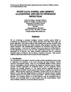
B. The Fuzzy Data Mining Algorithm It is important to note that a fuzzy rule can be of different orders. A first-order fuzzy rule can be defined to be a rule involving one linguistic term in its antecedent; a second-order rule can be defined to have two; and a third-order rule can be defined to have three linguistic terms, etc. Our approach is given in Fig. 1. 1) F1 = {first-order fuzzy rules}; 2) for (d = 2; |Fd – 1| ≠ φ; d + +) do 3) begin 4) T = {each linguistic term in the antecedent of l | l ∈ Fd – 1}; 5) forall ϕ composed of d elements in T do 6) calculate deg LwqLϕk using (2); 7) forall Lwq, Lϕk do 8) begin 9) if interesting(Lwq, Lϕk) then 10) Fd = Fd ∪ rulegen(Lwq, Lϕk); 11) end 12) end 13) F =
Fd ; �
d
Fig. 1. The fuzzy data mining algorithm.
To mine interesting first-order rules, our approach makes use of an objective interestingness measure introduced in Section C below. After these rules are discovered, they are stored in F1 (Fig. 1). Rules in F1 are then used to generate second-order rules that are then stored in F2. F2 is then used to generate third-order rules that are stored in F3 and so on for 4th and higher order. Our approach iterates until no higher order rule can be found.
The function, interesting(Lwq, Lϕk), computes an objective measure to determine whether the relationship between Lwq and Lϕk is interesting. If interesting(Lwq, Lϕk) returns true, a fuzzy rule is then generated by the rulegen function. For each rule generated, this function also returns an uncertainty measure associated with the rule (see Section D). All fuzzy rules generated by rulegen are stored in F that will then be used later for prediction or for the user to examine. C. Discovering Interesting Rules in Fuzzy Subsequences In order to decide whether a relationship between a linguistic term, Lϕk, and another linguistic term, Lwq, is interesting, we determine whether Pr( L wq | Lϕk ) =
sum of degrees to which records characteri zed by Lϕk and L wq
(3)
sum of degrees to which records characteri zed by Lϕk
where M =
sum of degrees to which records characterized by Lwq
� h
�� ���
γ Lwq Lϕk = 1 −
i =1
(4)
The significance of the difference can be objectively evaluated based on the idea of the adjusted residual [4-8] defined as:
γ Lwq Lϕk
(5)
where z LwqLϕk is the standardized residual [4-8] and is given by: z LwqLϕk =
deg LwqLϕk − eLwqLϕk
(6)
eLwq Lϕk
where eLwq Lϕk is the sum of degrees to which records are expected to be characterized by Lϕk and Lwq. It is defined as:
�
eLwqLϕk =
hu i =1
deg LwqLϕi
�
h i =1
M
M
�
�
��
(8)
Given that a linguistic term, Lϕk, is associated with another linguistic term, Lwq, we can form the following fuzzy rule.
L wq [ω LwqLϕk ]
where ω Lwq Lϕk is the weight of evidence measure that is Since the relationship between Lϕk and Lwq is interesting, there is some evidence for a record to be characterized by Lwq given it has Lϕk. The weight of evidence measure is defined in terms of an information theoretic measure known as mutual information. Mutual information measures the change of uncertainty about the presence of Lwq in a record given that it has Lϕk is, in turn, defined as: I (Lwq : Lϕk ) = log
Pr(L wq | Lϕk ) Pr(L wq )
(9)
Based on mutual information, the weight of evidence measure is defined in [4-8] as:
ω Lwq Lϕk = I (L wq : Lϕk ) − I ( = log
�
�
(L wi : Lϕk )) i≠q
Pr(Lϕk | L wq ) Pr(Lϕk |
(10)
L wi ) i≠q
deg LwiLϕk
(7)
and γ Lwq Lϕk is the maximum likelihood estimate [4-8] of the variance of z LwqLϕk and is given by:
i =1
deg LwiLϕk
defined as follows.
the relationship between Lϕk and Lwq interesting.
z LwqLϕk
� ��
h
distribution), we can conclude that the discrepancy between Pr(Lwq | Lϕk) and Pr(Lwq) is significantly different and hence the relationship between Lϕk and Lwq is interesting. Specifically, the presence of Lϕk implies the presence of Lwq. In other words, it is more likely for a record having both Lϕk and Lwq.
Lϕk
deg LwjLϕi . If this is the case, we consider
d LwqLϕk =
1−
M
u
j =1 i =1
deg Lwq Lϕi
� �� �� �� �� �� �� ��
If dL wq Lϕk > 1.96 (the 95 percentiles of the normal
M h
hu
D. Uncertainty Representation
is significantly different from Pr(Lwq ) =
�� �
ω Lwq Lϕk can be interpreted intuitively as a measure of the difference in the gain in information when a record with Lϕk characterized by Lwq and when characterized by other linguistic terms. The weight of evidence measure can be used to weigh the significance or importance of fuzzy rules. E. Predicting Unknown Values Using Fuzzy Rules Given a subsequence, d = (α1, …, αw) where αj ∈ [0, 1], j = 1, …, w, αw is the value to be predicted. d can be represented by a fuzzy subsequence, d’ = (β1, …, βw) where
βj is a set of order pairs, {(L1, µ L1 (α j ) ), …, (Lh, µ Lh (α j ) )}, j = 1, …, w. The value of αw is given by the value of βw. To predict the correct value of βw, our approach searches the fuzzy rules with Lwq ∈ L as consequents. For any combination of values, αϕ, w ∉ ϕ, of d, it is characterized by a linguistic term, Lϕk, to a degree of compatibility, λLϕk (d ) , for each k ∈ {1, …, hu}. Given those rules implying the assignment of Lwq, Lϕk L wq [ω LwqLϕk ] , for all k ∈ ζ ⊆ {1, …, hu}, the evidence for such assignment is given by:
ω L wqαϕ =
ω Lwq Lϕk ⋅ λLϕk (d )
�
k ∈ζ
(11)
Suppose that, of the w – 1 values excluding βw, only some combinations of them, β[1], …, β[i], …, β[l] with β[i] = {βj | j ∈ {1, …, w – 1}} are found to match one or more rules, then the overall weight of evidence for the value of βw to be assigned to Lwq is given by: l
ωq = �
i =1
ω Lwq β[ j ]
(12)
As a result, the value of βw is given by {(L1, ω1), …, (Lq, ωq), …, (Lh, ωh)}. In order to assign a crisp value to αw, the following method is used. Given linguistic terms L1, …, Lh and their overall weight of evidences ω1, …, ωh, let µ ′Lq (x ) be the weighted degree of membership of x ∈ [0, 1] to the fuzzy set Lq, q ∈ {1, …, h}. µ L′ q (x) is given by:
µ L′ q ( x ) = ω q ⋅ µ Lq ( x )
(13)
where x ∈ [0, 1] and q = 1, …, h. The defuzzified value, F −1 (
h �
Lq ) , which provides an appropriate value for αw, is
q =1
then defined as: �
F −1 (
1
h �
Lq ) = q =1
0 �
µ L′ 1 ∪...∪ Lh ( x) ⋅ xdx 1 0
µ L′ 1 ∪...∪ Lh ( x)dx
(14)
where µ ′X ∪Y ( x ) = max(µ ′X ( x), µ Y′ ( x)) for any fuzzy sets X and Y. V. PERFORMANCE ANALYSIS To evaluate the performance of our approach, we tested it on the property database provided by the Hong Kong office of a worldwide property valuation company. The property database is extracted from the data warehouse maintained by the company. It contains the details of all buy/sell
transactions of flats at Whampoa Garden in Hong Kong during the period between 1991 and 2000. Whampoa Garden, which is one of the largest private real estates in Hong Kong, has been developed into 12 separate phases and there are 88 residential towers comprising 10,431 flats. The database consists of 11,176 records in total. Each of these records represents a buy/sell transaction of a flat and is characterized by 11 attributes. Of these attributes, 3 are categorical and 8 are quantitative. These attributes are summarized in Table 1. TABLE 1. ATTRIBUTES IN THE property DATABASE.
Attribute TRAND PHASE BLOCK_NO FLOOR_NO DIRECT DERV_SIZE BUILD_AGE BW BEDRM LIVRM PRICE
Description Date of transaction Name of the phase at which the flat located Block number Floor number Direction Size of the flat Building age Size of bay window Number of bed rooms Number of living rooms Price of the flat
The domain expert from the company aims at predicting the value of PRICE of a flat based on other attributes. To perform this task, we first divided the property database into 10 partitions, D1, …, D10, where D1 contains the buy/sell transactions in 1991, D2 contains the buy/sell transactions in 1992, etc. We then discretized the domain of quantitative attributes into 5 intervals using [10] and made use of Apriori [3] to discover 9 sets of association rules, R1, …, R9, from the first 9 database partitions, D1, …, D9. After that, we scanned the 9 database partitions once to find the missing supports and confidences of the discovered association rules, R = R1 ∪ … ∪ R9. Finally, we applied the fuzzy data mining algorithm described in Section IV to discover a set of fuzzy rules, which represents the regularities about changes in the support and confidence of each association rule in R. Using the discovered fuzzy rules, we predicted how the support and confidence of each association rule in R changed. This resulted in a set of association rules, R′10 , such that the support and confidence of each rule in R′10 is predicted based on the changes in the association rules discovered in the time period between 1991 and 1999. We then used CBA [12] to predict the value of PRICE in each record in the last database partition, D10, using R′10 . Specifically, given a record in D10, CBA classifies it into one of the 5 intervals and the mid-point of this interval is considered as the value of PRICE predicted by CBA. In our experiments, we used the percentage error as a performance measure. Let N be the number of records in D10. For any record, τ ∈ D10, let tτ be the target value of PRICE in τ and oτ be the value predicted by CBA. The percentage error, error, is defined as
error =
tτ − oτ 1 N τ ∈D oτ 10
To further evaluate the performance of our approach, we used the association rules discovered in D9 (i.e., R9) to predict the value of PRICE in the records in D10. Furthermore, we also divided D10 into two datasets, one for training and the other for testing. The training dataset contains 80% of records in D10 and the testing dataset contains the remaining 20% of records. We then discovered a set of association rules, R10, from the training dataset and used these rules to predict the value of PRICE in the records in the testing dataset. This step is repeated ten times. It is important to note that the prediction of the value of PRICE in the records in the testing dataset based on the association rules discovered in the training dataset is the ideal case because the training and testing datasets are randomly selected from D10 and they are therefore homogeneous. All the experiments were performed on a Sun Ultra 5 workstation with 64 MB of main memory running Solaris 2.6. In our experiments, we set the minimum support to 1% and the minimum confidence to 50% for the mining of association rules. We also set the width of the sliding window, w, to 5. The experimental results are given in Table 2. TABLE 2. EXPERIMENTAL RESULTS ON THE property DATABASE.
Rule Set R9 R′10 R10
Percentage Error 16.7% 15.1% 14.2%
As shown in Table 2, the rule set produced by our approach (i.e., R′10 ) obtained better accuracy than the rule set discovered in D9 collected in 1999 (i.e., R9) in predicting the value of PRICE in the records in D10 collected in 2000. Although the performance of our approach is not as good as the ideal case (i.e., R10), the experimental results shown that our approach is able to improve the performance of a data mining algorithm by discovering and predicting the changes in rules over time. VI. CONCLUSIONS Existing data mining algorithms typically assume that the underlying associations hidden in the data are stable over time and they therefore discover association rules from the whole database. However, it is possible that the data characteristics and the associations change significantly in different time periods. Although it is an important problem, existing data mining algorithms have not taken these changes into consideration. In this paper, we introduced a fuzzy approach for mining and predicting how the association rules changed over time. To evaluate the performance of the proposed approach, we have applied it to a database containing all buy/sell transactions of flats in a large private real estate in Hong Kong during the period between 1991 and
2000. The experimental results shown that our approach is very effective in mining and predicting changes in association rules in such a way that it can improve the performance of existing data mining algorithms, especially when the discovered rules are used for classification (prediction). ACKNOWLEGMENTS The research was supported in part by PolyU Grant, AP209 and G-V918. REFERENCES [1] R. Agrawal, T. Imielinski, and A. Swami, “Mining Association Rules between Sets of Items in Large Databases,” in Proc. of the ACM SIGMOD Int’l Conf. on Management of Data, Washington D.C., 1993, pp. 207-216. [2] R. Agrawal and G. Psaila, “Active Data Mining,” in Proc. of the 1st Int’l Conf. on Knowledge Discovery and Data Mining, Montreal, Canada, 1995. [3] R. Agrawal and R. Srikant, “Fast Algorithms for Mining Association Rules,” in Proc. of the 20th Int’l Conf. on Very Large Data Bases, Santiago, Chile, 1994, pp. 487-499. [4] W.-H. Au and K.C.C. Chan, “An Effective Algorithm for Discovering Fuzzy Rules in Relational Databases,” in Proc. of the 7th IEEE Int’l Conf. on Fuzzy Systems, Anchorage, Alaska, 1998, pp. 1314-1319. [5] W.-H. Au and K.C.C. Chan, “FARM: A Data Mining System for Discovering Fuzzy Association Rules,” in Proc. of the 8th IEEE Int’l Conf. on Fuzzy Systems, Seoul, Korea, 1999, pp. 1217-1222. [6] W.-H. Au and K.C.C. Chan, “Classification with Degree of Membership: A Fuzzy Approach,” in Proc. of the 1st IEEE Int’l Conf. on Data Mining, San Jose, CA, 2001. [7] K.C.C. Chan and W.-H. Au, “Mining Fuzzy Association Rules,” in Proc. of the 6th Int’l Conf. on Information and Knowledge Management, Las Vegas, Nevada, 1997, pp. 209-215. [8] K.C.C. Chan and W.-H. Au, “Mining Fuzzy Association Rules in a Database Containing Relational and Transactional Data,” in A. Kandel, M. Last, and H. Bunke (Eds.), Data Mining and Computational Intelligence, New York, NY: Physica-Verlag, 2001, pp. 95-114. [9] D.W. Cheung, J. Han, V.T. Ng, and C.Y. Wong, “Maintenance of Discovered Association Rules in Large Databases: An Incremental Updating Technique,” in Proc. of the 12th Int’l Conf. on Data Engineering, New Orleans, Louisiana, 1996, pp. 106-114. [10] J.Y. Ching, A.K.C. Wong, and K.C.C. Chan, “Class-Dependent Discretization for Inductive Learning from Continuous and MixedMode Data,” IEEE Trans. on Pattern Analysis and Machine Intelligence, vol. 17, no. 6, pp. 1-11, 1995. [11] V. Ganti, J. Gehrke, R. Ramakrishnan, and W.-Y. Loh, “A Framework for Measuring Changes in Data Characteristics,” in Proc. of the 18th ACM SIGMOD-SIGACT-SIGART Symp. on Principles of Database Systems, Philadelphia, PA, 1999, pp. 126-137. [12] B. Liu, W. Hsu, and Y. Ma, “Integrating Classification and Association Rule Mining,” in Proc. of the 4th Int’l Conf. on Knowledge Discovery and Data Mining, New York, NY, 1998. [13] B. Liu, Y. Ma, and R. Lee, “Analyzing the Interestingness of Association Rules from the Temporal Dimension,” in Proc. of the 1st IEEE Int’l Conf. on Data Mining, San Jose, CA, 2001. [14] H. Mannila, H. Toivonen, and A.I. Verkamo, “Efficient Algorithms for Discovering Association Rules,” in Proc. of the AAAI Workshop on Knowledge Discovery in Databases, Seattle, Washington, 1994, pp. 181-192. [15] R. Srikant and R. Agrawal, “Mining Quantitative Association Rules in Large Relational Tables,” in Proc. of the ACM SIGMOD Int’l Conf. on Management of Data, Montreal, Canada, 1996, pp. 1-12.