FUZZY LOGIC DEDUCTION IN THE FRAME OF FUZZY ... - irafm

UNIVERSITY OF OSTRAVA FACULTY OF SCIENCE DEPARTMENT OF MATHEMATICS

FUZZY LOGIC DEDUCTION IN THE FRAME OF FUZZY LOGIC IN A BROADER SENSE

Ph.D. THESIS

AUTHOR: Anton´ın Dvoˇra´k SUPERVISOR: Prof. Ing. Vil´em Nov´ak, DrSc.

2003

´ UNIVERZITA V OSTRAVE ˇ OSTRAVSKA ˇ ´IRODOVEDECK ˇ ´ FAKULTA PR A KATEDRA MATEMATIKY

´ DEDUKCE V RAMCI ´ FUZZY LOGICKA ˇ S ˇ´IM SMYSLU FUZZY LOGIKY V SIR

´ DISERTACN ˇ ´I PRACE ´ DOKTORSKA

AUTOR: Anton´ın Dvoˇra´k ´ VEDOUC´I PRACE: Prof. Ing. Vil´em Nov´ak, DrSc.

2003

Summary An important role in fuzzy logic and fuzzy control is played by linguistic descriptions, i.e. finite sets of IF-THEN rules. These rules often include so-called evaluating linguistic expressions – natural language expressions which characterize a position on an ordered scale, usually on a real interval. Examples of evaluating linguistic expressions are small, more or less medium, approximately 20 etc. Given a linguistic description of a process, situation, environment etc., and an observation, i.e. a value measured in some concrete situation, the task is to determine the conclusion by some plausible method. This thesis proposes a methodology for dealing with the above-described situation and studies its properties. The basis for it is fuzzy logic in a narrow sense with evaluated syntax [27]. IF-THEN rules are understood as linguistically expressed logical implications. We consistently distinguished three levels of study – linguistic, syntactic and semantic. The meaning of evaluating linguistic expression is characterized on syntactic level by its intension and on semantic level by a class of its extensions. First we investigate properties that a formal theory aimed at the characterization of evaluating linguistic expressions should have. We call the theory which fulfills these properties the theory of evaluating expressions. Further we use theories of evaluating expressions for the determination of the formal theory which characterizes the meaning of a linguistic description, called the theory of linguistic description. The central part of our thesis is a study of fuzzy logic deduction. It uses the theory of linguistic description and another theory describing an observation for determination of conclusion by means of formal proving in clearly defined logic. First we prove some general properties of fuzzy logic deduction and then we study one important aspect of the work with linguistic descriptions, so-called inconsistencies. Last part of our thesis is devoted to a situation in which an observation is given as a crisp number. Keywords: Logical deduction, intension, linguistic description, IF-THEN rules, fuzzy logic.

5

Anotace D˚ uleˇzitou roli ve fuzzy logice a fuzzy regulaci hraj´ı jazykov´e popisy, tj. koneˇcn´e ˇ mnoˇziny JESTLIZE-PAK pravidel. V mnoha pˇr´ıpadech tyto pravidla obsahuj´ı tzv. evaluaˇcn´ı jazykov´e v´ yrazy – v´ yrazy pˇrirozen´eho jazyka charakterizuj´ıc´ı pozici na uspoˇra´dan´e ˇsk´ale, obvykle na intervalu re´aln´ ych ˇc´ısel. Pˇr´ıklady evaluaˇcn´ıch jazykov´ ych v´ yraz˚ u jsou mal´ y, v´ıce m´enˇe stˇredn´ı, pˇribliˇznˇe 20 apod. M´ame-li zad´an jazykov´ y popis nˇejak´eho procesu, situace, prostˇred´ı apod. a pozorov´ an´ı, tedy hodnotu namˇeˇrenou v nˇejak´e konkr´etn´ı situaci, je naˇs´ım u ´kolem urˇcit z´avˇer pomoc´ı nˇejak´e vˇedecky podloˇzen´e metody. Tato disertace navrhuje metodologii popisuj´ıc´ı tuto situaci a studuje jej´ı vlastnosti. Z´akladem pro tuto metodologii je fuzzy logika v uˇzˇs´ım smyslu s ohodnocenou ˇ syntax´ı [27]. JESTLIZE-PAK pravidla jsou ch´ap´ana jako jazykovˇe vyj´adˇren´e logick´e implikace. D˚ uslednˇe rozliˇsujeme tˇri u ´rovnˇe pr´ace s jazykov´ ymi v´ yrazy – jazykovou, syntaktickou a s´emantickou. V´ yznam evaluaˇcn´ıho jazykov´eho v´ yrazu je vyj´adˇren jeho intenz´ı na syntaktick´e u ´rovni a tˇr´ıdou jeho extenz´ı na u ´rovni s´emantick´e. Nejprve jsou zkoum´any podm´ınky, kter´e mus´ı splˇ novat form´aln´ı teorie zamˇeˇren´a na charakterizaci evaluaˇcn´ıch jazykov´ ych v´ yraz˚ u. Teorii splˇ nuj´ıc´ı tyto podm´ınky u. Teorie evaluaˇcn´ıch v´ naz´ yv´ame teori´ı evaluaˇcn´ıch v´yraz˚ yraz˚ u jsou d´ale pouˇzity k sestrojen´ı form´aln´ı teorie charakterizuj´ıc´ı v´ yznam jazykov´eho popisu, tzv. teorie ´ jazykov´eho popisu. Ustˇredn´ı ˇca´st´ı t´eto disertace je studium fuzzy logick´e dedukce. Zde je pouˇzita teorie jazykov´eho popisu spolu s dalˇs´ı teori´ı popisuj´ıc´ı pozorov´an´ı k urˇcen´ı z´avˇeru pomoc´ı form´aln´ıho dokazov´an´ı v jednoznaˇcnˇe definovan´e logice. Nejprve jsou uk´az´any obecn´e vlastnosti fuzzy logick´e dedukce, d´ale pak studujeme jeden v´ yznaˇcn´ y aspekt pr´ace s jazykov´ ymi popisy, tzv. nekonzistence v jazykov´ ych popisech. Z´avˇereˇcn´a ˇca´st disertace je vˇenov´ana fuzzy logick´e dedukci s pozorov´an´ım ve formˇe re´aln´eho ˇc´ısla. ˇ Kl´ıˇ cov´ a slova: Logick´a dedukce, intenze, jazykov´ y popis, JESTLIZE-PAK pravidla, fuzzy logika.

6

Preface Fuzzy logic is an important tool for the modeling of vagueness. The importance of vagueness and its transmission and propagation in human thinking and everyday human communication is indisputable. Fuzzy logic offers powerful and transparent methodology which allows to describe and model vague phenomena. The applications of fuzzy logic in control, decision making and other areas are numerous and successful. However, from the emergence of fuzzy logic and fuzzy set theory in the 1960’s up to the 1990’s objections often occurred reproaching that fuzzy logic lacked solid mathematical foundations. These objections lost ground at the end of the 1990’s when the important books [13], [27] and some others appeared. However, there are still areas in mathematical foundations of fuzzy logic that have to be investigated. The aim of this thesis is to propose and investigate mathematical model of the meaning of evaluating linguistic expressions, i.e. linguistic expressions which characterize a position on an ordered scale. Further, the structure and meaning of linguistic descriptions, i.e. finite sets of IF-THEN rules are investigated. These meanings are described separately on syntactic and semantic levels. The concepts introduced and results obtained are then used in the central part of this thesis, namely in the investigation of fuzzy logic deduction. The deduction is performed on syntactic level as a formal proving in some formal theory. An important concept of inconsistency of linguistic description is discussed and its two definitions are proposed. Finally, fuzzy logic deduction with crisp observations, which is important in applications of fuzzy logic, is also investigated. The methodology and results obtained in this thesis are, or will be, used in the software system LFLC 2000 developed in our Institute for Research and Applications of Fuzzy Modeling. LFLC 2000 is a software system which allows to design, test and apply linguistic descriptions. It proved itself to be useful also in practical applications. 7

I want to thank my supervisor Prof. Vil´em Nov´ak for his support, permanent encouragement and working conditions he created in Institute for Research and Applications of Fuzzy Modeling. I would also like to thank colleagues from our Institute and my parents. Ostrava, April 2003

Anton´ın Dvoˇr´ak

8

Table of Contents Summary

5

Anotace

6

Preface

7

Table of Contents

9

List of Figures

12

List of Symbols

13

1 Introduction

15

2 Current State of Research 21 2.1 Nov´ak’s approach . . . . . . . . . . . . . . . . . . . . . . . . . . . . . 21 2.2 H´ajek’s approach . . . . . . . . . . . . . . . . . . . . . . . . . . . . . 22 2.3 IF-THEN rules as fuzzy logic programs . . . . . . . . . . . . . . . . . 23 3 Preliminaries 3.1 Logical preliminaries . . . . . . . . . . . . . . . . . . . . 3.1.1 The structure of truth values . . . . . . . . . . . 3.1.2 Language and syntax of FLn . . . . . . . . . . . . 3.1.3 Semantics of FLn . . . . . . . . . . . . . . . . . . 3.1.4 Many-sorted fuzzy predicate logic . . . . . . . . . 3.1.5 Fuzzy theories, provability degrees, completeness . 3.1.6 Independence of formulas . . . . . . . . . . . . . 3.1.7 Isomorphism of models in fuzzy logic . . . . . . . 3.1.8 Theories with fuzzy equality . . . . . . . . . . . . 9

. . . . . . . . .

. . . . . . . . .

. . . . . . . . .

. . . . . . . . .

. . . . . . . . .

. . . . . . . . .

. . . . . . . . .

25 25 25 27 28 30 30 32 33 34

3.2

3.3

3.4

Linguistic preliminaries . . . . . . . . . . 3.2.1 Linguistic predications . . . . . . 3.2.2 Evaluating linguistic expressions . Meaning of linguistic expressions . . . . 3.3.1 Intensions and extensions . . . . 3.3.2 Possible worlds . . . . . . . . . . 3.3.3 Meaning of evaluating expressions Other preliminaries . . . . . . . . . . . . 3.4.1 Tolerance relations . . . . . . . . 3.4.2 Unimodality . . . . . . . . . . . .

. . . . . . . . . .

. . . . . . . . . .

. . . . . . . . . .

. . . . . . . . . .

. . . . . . . . . .

. . . . . . . . . .

. . . . . . . . . .

4 Theories for Modeling of the Meaning of Evaluating pressions 4.1 Definition of theory T ev . . . . . . . . . . . . . . . . 4.2 Canonical possible worlds . . . . . . . . . . . . . . . 4.3 Extended theories . . . . . . . . . . . . . . . . . . . . 4.4 Theories T ev and T evx with fuzzy equality . . . . . .

. . . . . . . . . .

. . . . . . . . . .

. . . . . . . . . .

. . . . . . . . . .

. . . . . . . . . .

. . . . . . . . . .

. . . . . . . . . .

. . . . . . . . . .

. . . . . . . . . .

34 34 35 36 36 37 38 38 38 39

Linguistic Ex. . . .

44 44 49 50 56

5 Linguistic Descriptions 5.1 Linguistic level . . . . . . . . . . . . . . . . . . . . . . . . . . . . . . 5.2 Level of syntax . . . . . . . . . . . . . . . . . . . . . . . . . . . . . . 5.3 Level of semantics . . . . . . . . . . . . . . . . . . . . . . . . . . . . .

57 57 58 61

. . . .

. . . .

. . . .

. . . .

. . . .

. . . .

. . . .

. . . .

6 Fuzzy Logic Deduction 62 6.1 Basic scheme . . . . . . . . . . . . . . . . . . . . . . . . . . . . . . . 62 6.2 Inconsistencies in linguistic description . . . . . . . . . . . . . . . . . 68 6.3 Alternative approach to inconsistency of linguistic descriptions . . . . 72 7 An 7.1 7.2 7.3 7.4

Application — Deduction with Crisp Observations General properties . . . . . . . . . . . . . . . . . . . . . . . . The operation Suit . . . . . . . . . . . . . . . . . . . . . . . . The algorithm of fuzzy logic deduction with crisp observations The behavior of fuzzy logic deduction with crisp observations .

. . . .

. . . .

. . . .

. . . .

79 80 82 85 90

8 Conclusion

93

List of Author’s Publications

95

10

Bibliography

97

Index

100

11

List of Figures 3.1

Example of unimodal function. . . . . . . . . . . . . . . . . . . . . . 39

3.2

Three types of unimodal functions. . . . . . . . . . . . . . . . . . . . 41

6.1

Situation a1 ) from the proof of Theorem 6.15. . . . . . . . . . . . . . 72

7.1

The function ha1 , c2 , d2 i from the proof of Lemma 7.10. . . . . . . . . 87

7.2

Continuity of DEEs defuzzification method. . . . . . . . . . . . . . . 89

12

List of Symbols ∃, existential quantifier, 27 ∀, universal quantifier, 27 ∼ =, isomorphism of models, 33 ≈, fuzzy equality, 34, 69 ⊂ , fuzzy subset of, 21 ∼ &, L Ã ukasiewicz conjunction, 27 ∇, L Ã ukasiewicz disjunction, 27 ∧ , conjunction, 27 ∨ , disjunction, 27 ⇒ , implication, 27 ⇔ , equivalence, 27 ¬ , negation, 27 6⇔ , nonequivalence, 53 ⊗, L Ã ukasiewicz t-norm, 26 ⊕, L Ã ukasiewicz t-conorm, 26 →, L Ã ukasiewicz implication, 27 ↔, L Ã ukasiewicz biresiduation, 29 ¬, L Ã ukasiewicz negation, 26 |=a , degree of truth, 31 `a , provability degree, 31 ≺, order relation for Suit operation, 83 An, antecedent, 57 A0hxi , intension of an observation, 62 Ae , intension in extended theories, 51 α ˜ G , intensional mapping, 45 B0 , conclusion, 63 β˜G , second intensional mapping, 51 Cu , set of all unimodal functions, 39 c0 , threshold for operation Suit, 83

DEEs, defuzzification of evaluating expressions, 86 d, metric, 81 d(s1 , s2 ), provability degree of nonequality, 69 Ext, extension, 38 e, evaluation of free variables, 29 FJ , set of formulas, 27 FLb, fuzzy logic in broader sense, 57 FLn, fuzzy logic in narrow sense, 25 G, set of unary predicate symbols, 45 GVE , interpretation of predicate G in an extended possible world, 51 γG , functions adjoined to α ˜ G , 45 Int, intension, 38 J(T ), language of theory T , 30 J(TI ), language of theory TI , 58 K, set of all continuous functions, 86 L, set of truth values, 26 L, L Ã ukasiewicz MV-algebra, 26 LAx, fuzzy set of logical axioms, 30 LD, input-output mapping for fuzzy logic deduction, 90 I LD , linguistic description, 57 M , set of closed terms, 17 m, bijection between S and G, 45 mt , maximal value of operation p, 83 Mean(A), meaning of A, 38 P, set of predicate symbols, 33 13

p, auxiliary operation for Suit, 83 Π, unimodal function of type Π, 40 R, IF-THEN rule, 57 S, unimodal function of type S, 40 S, set of simple eval. expressions, 45 Shxi , set of intensions, 48 SAx, fuzzy set of special axioms, 30 Succ, succedent, 57 Suit, suitable linguistic expression operation, 83 0 T , theory representing an observation, 62 TD , deduction theory, 62 TD≈ , theory TD with nonequality axioms, 69 TI , theory of linguistic description, 59 TIA , antecedent part of TI , 60 TIE , extended theory TI , 60 TIS , succedent part of TI , 60 T ev , theory of evaluating expressions, 45 evx T , extended theory, 51 T≈ev , theory of evaluating expressions with fuzzy equality, 56 (z) t , term corresponding to real number z, 47 uni, first type of unimodality relation, 40 unim , second type of unimodality relation, 40 T ev uni , first type of unimodality over eval. expressions, 48 T ev unim , second type of unimodality over eval. expressions, 48 Val(wA ), value of evaluated proof, 31 VC , canonical possible world, 49

VE , extended possible world, 51 wA , evaluated proof of formula A, 31 Z, unimodal function of type Z, 40

14

Chapter 1 Introduction This thesis is a study of one approach to approximate reasoning over a set of IFTHEN rules called fuzzy logic deduction. The novelty of our approach lies in the fact that the inference is performed on syntactic level as a formal proving in a formal logical system. This is a substantial difference in comparison with the classical method, namely the compositional rule of inference (see [35, 13]), which is defined on the semantic level. Fuzzy logic has been, from its boom in 1980’s till now, one of the most widely used methodologies for dealing with the phenomenon of indeterminacy. Its applications are numerous, mainly in the fields of control and optimization, but also in other areas, such as clustering, pattern recognition, expert systems, economy, psychology etc. The phenomenon which could be most successfully modeled by means of fuzzy logic is called vagueness. It is one of the facets of the above-mentioned indeterminacy (another is uncertainty, that emerges due to lack of knowledge about the occurrence of some event). The vagueness occurs in the process of grouping together objects which have some property φ (e.g. tallness). Quite often is such a grouping imprecise, there exist borderline elements, i.e. elements which have the property φ only to some extent. There are various approaches trying to model this phenomenon, inside or outside of classical logic (see e.g. [15]). One of the important properties of vagueness, which we will often use in the following, is its continuity. It means that for similar objects should also the extent in which they have the property φ be similar. In a great part of applications of fuzzy logic, so called IF-THEN rules are used. They have the form IF X is A THEN Y is B where X, Y are linguistic variables and

15

A, B are linguistic expressions. Most widely used are so-called evaluating linguistic expressions, which express the position on some ordered scale, most often on an interval of real numbers. However, in practice there are usually more than one linguistic variables on the left side of IF-THEN rule. IF-THEN rules are then grouped into (finite) set, called rulebase (we will call it linguistic description). This set of IF-THEN rules is a natural way to catch human knowledge about some process, situation etc. Then, given some observation (in the form of real number, interval of real numbers, linguistic expression, fuzzy set etc.), we need to determine a conclusion. If the rulebase is comprehensible to humans, then the conclusion should correspond with human intuition - should be similar to the conclusion carried out by humans. There was a lot of discussions in the literature about the suitability of fuzzy logic for modeling of the phenomenon of vagueness and of the theoretical background of fuzzy logic and, namely, of fuzzy control. In recent years a lot of progress in this field has been done (as the most important contributions let us name books [14, 27, 11], see also Chapter 2). However, there is still a lot of open problems and not-fullyunderstood areas. Our thesis tries to contribute to this area of research. We can distinguish two approaches in the general theory of fuzzy IF-THEN rules. The first one, called fuzzy approximation (see [30, 31]) uses linguistic form of the IF-THEN rules as a motivation for finding special formulas called disjunctive (DNF) and conjunctive (CNF) normal forms. The goal is to approximate a function described by IF-THEN rules in some model with prescribed accuracy. The second possibility is to take the set of IF-THEN rules as the set of genuine linguistic expressions, find their logical interpretation and work with this interpretation inside some formal logical theory. This approach is based on fuzzy logic in narrow sense with evaluated syntax. This thesis focuses on the second approach. We will show the possible interpretation of linguistic description and the way how logical deduction based on it can be performed. To be able to perform this task, we should first study the modeling of the meaning of linguistic expressions occurring in these IF-THEN rules. We restrict ourselves to so-called simple evaluating linguistic expressions (such as medium, more or less small, extremely big etc.). This class of expressions is most widely used in practice. We then use the same methodology for modeling of the meaning of one IF-THEN rule and sets of them. We will always carefully distinguish three levels on which we are working, namely 16

linguistic (e.g linguistic expressions such as small), syntactic (e.g. intensions of these expressions, formal theories etc.) and semantic (extensions of linguistic expressions in some possible world). We will focus our attention mainly on the syntactic level, because in the inclusion of this level lies the novelty of our approach. Moreover, all results obtained in syntactic level are automatically (due to the correctness of fuzzy predicate logic) valid in all possible worlds. First, in Chapter 2, we review some approaches to the study of IF-THEN rules and deduction over sets of them. We briefly describe the approaches of H´ajek, Nov´ak and Vojt´aˇs. In Chapter 3 we introduce necessary preliminaries. Besides the material concerning predicate first-order fuzzy logic, we will also add linguistic preliminaries and review some other notions used in further chapters (namely tolerance relations and real unimodal functions of one variable). In Chapter 4 we start to study formal theories for the modeling of so-called evaluating linguistic expressions. We call such theories theories of evaluating expressions. We will not try to determine one (“unique”, “best”) theory, we rather postulate several axioms every such a theory should obey. The basis for our study is first-order fuzzy logic in a narrow sense with evaluated syntax [27]. On the syntactic level, the meaning of an evaluating expression is characterized by its intension. We assign to evaluating expression A a formula A(x) with one free variable. The intension of A is then the set of evaluated formulas ¯ n o ± ˜ A (t) Ax [t]¯¯ t ∈ M, α Int(A) = Ahxi = α ˜ A (t) ∈ L (1.1) where M is a set of closed terms, L is a set of truth values and α ˜ A (t) are syntactic evaluations of instances of formula A(x). Syntactic evaluations could be obtained as provability degrees of the respective instances of A(x) in some theory [21]. To every considered simple evaluating expression Ai we add a predicate symbol Gi to our formal language. Instances of atomic formulas Gi,x [t] together with their syntactic evaluations α ˜ Gi (t) form an essential part of the theory of evaluating expressions denoted by T ev (the theory should also include some technical axioms which assure correct behavior of equality predicate etc.). All simple evaluating linguistic expressions are treated uniformly, i.e. we are not considering any structure over the set of them (e.g. linguistic hedges). But, if there is some theory where hedges are taken into account (like in e.g. [21]), it can be translated into our system and we can study its properties. This means that our level of study is lower, but at the same time more general than in [21]. 17

We will prove that theories of evaluating expressions indeed exist (Lemma 4.2). On the semantic level, the meaning of an evaluating expression is modeled by its extension – satisfaction set of formula A(x) in a model V of a theory T ev : n o ± ¯¯ V(A(v/x)) ExtV (A) = v¯ v ∈ V where V is a support of the structure V. Models of T ev are also called possible worlds. Then we will study special class of models of such theories, so-called canonical possible worlds (Section 4.2). These structures have a property that truth values of instances of formulas Ax [t] from (1.1) coincide with syntactic evaluations of these instances. If such a structure does not exist for some theory of evaluating expressions, then the effort of its forming would be futile, because we never attain a proper correspondence between syntactic and semantic levels. Theorem 4.7 will show that under some conditions, which are usually fulfilled, such structures exist. A well-known property of the relationship between syntax and semantics in (not only) fuzzy logic is that the truth value of a formula A in some model D denoted by D(A) is, in general, greater than or equal to its provability degree. The equality of these two quantities is attained for complete theories. Therefore, it is possible that the theory T ev mentioned above can have a model D? in which all truth degrees for all instances of atomic formulas Gi,x [t] have value 1 and on that account they are in D? undistinguishable. We propose (in Section 4.3) to restrict the range of these ± truth values by means of an addition of axioms of the form {β˜Gi (t) ¬ Gi,x [t]}, where it should hold that α ˜ Gi (t) ⊗ β˜Gi (t) = 0. We call such theories extended theories of evaluating expressions T evx . We will again define a structure (called extended possible world ) which plays similar role as the canonical possible world above. We will prove that such structures exist (Theorem 4.13) and show some properties of these models. At the end of Chapter 4 there is a short section concerning theories of evaluating expressions with fuzzy equality. In the following Chapter 5 we study linguistic descriptions, i.e. sets of IF-THEN rules. We again start on linguistic level, then we proceed to syntactic (Section 5.2) and semantic (Section 5.3) levels. On syntactic level we form an intension of one IFTHEN rule Rhx,yi . From these intensions we form a theory of linguistic description TI . On semantic level, we define a canonical possible world for the theory TI and show that it always exists (Theorem 5.6). Chapter 6 “Fuzzy logic deduction” is the central part of our thesis. We will introduce (in Section 6.1) its so-called basic schema. The deduction is performed on syntactic level and the conclusion is obtained in the form of closed instances of atomic 18

0 formulas By [s] and their respective provability degrees α ˜B (s) in the theory TD . This theory is formed as a union of the theory TI introduced in the previous chapter, and of a theory T 0 representing an observation. Theorem 6.5 (proved already in [27]), Theorem 6.1) shows how these provability degrees can be computed. We then show some general properties of our fuzzy logic deduction (Theorems 6.6, 6.9 and Corollary 6.10). It is interesting that these results show that our fuzzy logic deduction satisfies the conditions imposed by C. Cornelis and E. E. Kerre in [4] on general inference procedures.

When we postulate our basic schema of fuzzy logic deduction, we are able to investigate its properties from several viewpoints. In our thesis, we focus on the description of so-called inconsistencies in linguistic descriptions. By inconsistency we understand the situation when there are identical (or similar) antecedents and different consequents present in linguistic description. First, in Section 6.2 we take a negation of the standard formula defining the condition which a relation should fulfil to be a function and rewrite it into our formalism, using fuzzy equality. This notion of inconsistency is called ≈-inconsistency. Then, in Section 6.3 we present another approach. We use a notion of unimodal 0 function and say that some theory TD is u-inconsistent if the function α ˜B (s) mentioned above is not unimodal (more precisely, we should consider the real function 0 γB0 associated to α ˜B ). In this way we can describe this type of inconsistency for one observation. Then we generalize this notion to be able to describe inconsistency for all sensible observations. This more general notion is called u? -inconsistency. The dual notion is u? -consistency. We will show necessary and sufficient conditions for this type of consistency of linguistic description in Theorem 6.22. Finally, in Chapter 7 we apply the methodology and results of previous chapter to the situation, when a crisp number measured in some possible world is taken as an observation. In particular, we study a case when one IF-THEN rule is taken and the deduction is performed by means of this most suitable rule. To this purpose we introduce an operation Suit, which selects the most suitable linguistic expression, and, consequently, also the most suitable IF-THEN rule for the given observation. We also introduce special defuzzification method DEEs (defuzzification of evaluating expressions) and study some of its properties, namely its (dis)continuity. Then we can investigate a real function LD which describes the overall behavior of the algorithm of fuzzy logic deduction with crisp observations. We conclude that this function is piece-wise continuous. This result is then explained and discussed. 19

Author’s contribution Here I summarize my contribution in this thesis. 1. In Chapter 3: the definition of unimodal function and its properties (Section 3.4.2). 2. All definitions and results in Chapter 4. 3. The definition of theory TI in Section 5.2 and the definition of canonical possible world there and relevant results. 4. In Chapter 6: a formalization of a basic schema of fuzzy logic deduction and theorems in Section 6.1 (with exception of Theorem 6.5), concepts and results concerning two approaches to inconsistencies of linguistic descriptions (Sections 6.2 and 6.3). 5. In Chapter 7: a formalization of the operation Suit (Section 7.2), a formalization and results concerning the defuzzification operation DEEs and the overall behavior of fuzzy logic deduction with crisp observations (Sections 7.3 and 7.4). Results included in this thesis have not been published yet. Several definitions and results from Chapters 4, 5 and 6 were included in submitted paper [10] and accepted paper [9] (where a part of the content of Chapter 7 in a preliminary form is included).

20

Chapter 2 Current State of Research In this section we summarize several approaches to the approximate inference and analysis of IF-THEN rules in logical setting. From our point of view, the most important sources are books [27], Chapter 6 of which is most inspiring for our approach, further, book [13], where in Chapter 7 “On Approximate Inference” there is described approach and properties of approximate inference in L Ã ukasiewicz predicate logic with classical (non-evaluated) syntax. Another sources are papers [3, 34] and book [11]. Let us first review the traditional formulation of Zadeh’s compositional rule of inference [35, 13], which served as a basis of the study and applications of fuzzy IF-THEN rules. Let DX and DY be nonempty sets. Then: From ‘X is A’ and ‘(X, Y ) is R’ infer ‘Y is B’ if for all v ∈ DY , rB (v) = sup (rA (u) ? rR (u, v))

(2.1)

u∈DX

where ? is a continuous t-norm, rA ⊂ DX and rB ⊂ DY are fuzzy sets and ∼ ∼ rR ⊂ DX × DY ∼ is a binary fuzzy relation.

2.1

Nov´ ak’s approach

Here we present only main ideas, a more detailed treatment will be included in the foregoing sections. The novelty of his approach lies in the fact that, unlikely as in the classical compositional rule of inference, the main portion of inference process is 21

performed on syntactic level. The inference is, in his approach, the formal proving in exactly defined formal system. Also, the stress is put on the analysis of the meaning of linguistic expressions. He introduced the notions of intension, extension and possible world, well-known from the field of philosophical logic and introduced originally by Rudolf Carnap. Here, intension is defined on syntactic level. A formal model of intension is socalled multiformula, i.e. a fuzzy set of instances of evaluated formulas. Extension is an interpretation of intension in some specific structure (possible world). A linguistic expression has one intension and a class of extensions, one in every possible world. This approach supposes the existence of a sufficiently rich set of closed terms in the formal language. These terms are understood as some prototypical formal objects and they are substituted to formulas assigned to linguistic expressions. Intensions can be also considered as some prototypical interpretations, which restrict (from below) truth functions of extensions.

2.2

H´ ajek’s approach

H´ajek studies IF-THEN rules and approximate inference in BL∀, i.e. basic predicate logic. The main difference between Nov´ak and H´ajek approach lies in the fact that H´ajek incorporates in the language I only one object constant for each sort, which is in a model interpreted as an actual value of the variables X and Y (called variates there). The expression ‘X is A’ is then translated into predicate logic as an atomic formula A(X). An IF-THEN rule ‘IF X is A THEN Y is B’ may be interpreted as A(X) ⇒ B(Y ). Hence, the language I further contains unary predicate symbols A and B, and a binary predicate symbol R. Let D be a structure for the language I. The compositional rule of inference is expressed by the condition that formula Comp := (∀y)(B(y) ⇔ (∃x)(A(x) & R(x, y)) is 1-true in the model D. Then two particular cases of the formula Comp are studied. First, for Zadeh’s Generalized modus ponens (where the relation R from (2.1) is defined as rR (u, v) = rA (u) → rB (v), and → is the residuum of t-norm ?) CompM P := (∀y)(B ? (y) ⇔ (∃x)(A? (x) &(A(x) ⇒ B(y)))) and it is showed that BL∀ proves (CompM P & A? (X) &(A(X) ⇒ B(Y ))) ⇒ B ? (Y ). 22

(2.2)

Second, generalized conjunctive rule, where the relation R from (2.1) is defined as rR (u, v) = rA (u)&rB (v): CompCR := (∀y)(B ? (y) ⇔ (∃x)(A? (x) & A(x) & B(y))) and it is showed that BL∀ proves (CompCR & A? (X) &(A(X) & B(Y ))) ⇒ B ? (Y )

(2.3)

In the second part (Chapter 7.3) are X and Y also unary predicates and the assertion ‘X is Ai ’ is in the syntactic level translated into formula (∀x)(X(x) ⇒ A(x)) (or briefly X ⊆ A). This corresponds to a situation when actual values of variables are given not as crisp numbers, but only vaguely (as fuzzy sets). Then, an alternative composition for generalized modus ponens is the formula CompM P A := (∀y)(B ?? (y) ⇔ ((∀x)(A? (x) ⇒ A(x)) ⇒ B(y))). Then BL∀ proves CompM P A &((X ⊆ A? ) &((X ⊆ A) ⇒ (Y ⊆ B))) ⇒ (Y ⊆ B ?? ).

(2.4)

Formulas (2.2), (2.3) and (2.4) can be visualized as deduction rules, for example formula (2.2) as CompM P , A? (X), A(X) ⇒ B(Y ) B ? (Y ) which can be read as: If CompM P , A? (X) and A(X) ⇒ B(Y ) are 1-true in a given structure D, then B ? (Y ) is 1-true in D. This approach is the extensional one, because the meanings of linguistic expressions are modeled only on the semantic level. However, it also shows some general properties of inference valid in all models.

2.3

IF-THEN rules as fuzzy logic programs

Vojt´aˇs [34] treats IF-THEN rules in the framework of fuzzy logic programming without negation. In his system he uses various truth functions for conjunction, disjunction and implication; and also aggregation operations. He introduces a notion 23

of fuzzy theory as a partial mapping assigning to formulas rational numbers from (0, 1]. Then, many valued modus ponens is introduced by a schema (B, x), (B ⇒ A, y) A, mp⇒ (x, y) where x, y are axiomatically assigned truth values of formulas B and B ⇒ A, respectively, and mp⇒ is a function calculating truth value of the answer A. This function has to be a truth function of a conjunction (but it need not to be a truth function of conjunctions present in the language). Then the semantics is defined and the completeness of this system is showed. Gerla in his book [11] studies fuzzy logic mainly from the point of view of fuzzy closure operators. In Chapter 10 “On Approximate Inference” he transforms a set of IF-THEN rules to a fuzzy program.

24

Chapter 3 Preliminaries 3.1

Logical preliminaries

The formal system we are working in is fuzzy logic in a narrow sense with evaluated syntax (FLn). Main source here is the book [27], Chapter 4. We recall here the main points of this formal system, for the details we refer to the above-mentioned book.

3.1.1

The structure of truth values

The two most important algebraic structures for our system of fuzzy logic, used as algebras of truth values, are residuated lattices and MV-algebras. Definition 3.1 A residuated lattice is an algebra L = hL, ∨, ∧, ⊗, →, 0, 1i such that (i) hL, ∨, ∧, 0, 1i is a lattice with the ordering defined using the operations ∨, ∧, and 0, 1 are its least and greatest elements, respectively, (ii) hL, ⊗, 1i is a commutative monoid, i.e. ⊗ is commutative and associative operation with the identity a ⊗ 1 = a, (iii) it holds that a ⊗ b ≤ c iff a ≤ b → c 25

i.e. the operation → is a residuation operation with respect to ⊗. It holds that the operation → is antitonic in the first and isotonic in the second variable. Definition 3.2 An MV-algebra is an algebra L = hL, ⊗, ⊕, ¬, 0, 1i in which the following identities are valid: a ⊕ b = b ⊕ a,

a ⊗ b = b ⊗ a,

a ⊕ (b ⊕ c) = (a ⊕ b) ⊕ c,

a ⊗ (b ⊗ c) = (a ⊗ b) ⊗ c,

a ⊕ 0 = a,

a ⊗ 1 = a,

a ⊕ 1 = 1,

a ⊗ 0 = 0,

a ⊕ ¬a = 1,

a ⊗ ¬a = 0,

¬(a ⊕ b) = ¬a ⊗ ¬b,

¬(a ⊗ b) = ¬a ⊕ ¬b,

a = ¬¬a,

¬0 = 1,

¬(¬a ⊕ b) ⊕ b = ¬(¬b ⊕ a) ⊕ a. Lattice operations in an MV-algebra can be introduced as follows: a ∨ b = ¬(¬a ⊕ b) ⊕ b,

a ∧ b = ¬(¬a ∨ ¬b).

Residuation in an MV-algebra can be defined as a → b = ¬a ⊕ b. It holds that every MV-algebra is a residuated lattice, and that a residuated lattice is an MV-algebra iff (a → b) → b = a ∨ b. The fuzzy logic in a narrow sense with evaluated syntax is based on L Ã ukasiewicz MV-algebra L of truth values: L = hL, ⊗, ⊕, ¬, 0, 1i where the set of truth values is L = [0, 1], with standard ordering and L Ã ukasiewicz operations ⊗, ⊕ and ¬, defined as follows: a ⊗ b = max(a + b − 1, 0), 26

(3.1)

a ⊕ b = min(a + b, 1),

(3.2)

¬a = 1 − a

(3.3)

and for a, b ∈ L. Residuation in L Ã ukasiewicz MV-algebra is given by a → b = max(1 − a + b, 0).

(3.4)

The following simple lemma will be used in Chapter 6. Lemma 3.3 Let L be L Ã ukasiewicz MV-algebra, a, b ∈ L. If b < a then ¬b ⊗ a > 0.

proof: ¬b ⊗ a = (1 − b + a − 1) ∨ 0 = (a − b) ∨ 0. If b < a then b − a > 0. 3.1.2

2

Language and syntax of FLn

The language J of FLn consists of the following: (i) Countable set of object variables x1 , x2 , . . . . (ii) Set of object constants ui , i ∈ I. (iii) Finite or countable set of function symbols f, g, . . . together with their arities. (iv) Nonempty finite or countable set of predicate symbols P, Q, . . . together with their arities. (v) Logical constants {a | a ∈ L}. (vi) Symbols ⇒ and ∀ for implication and universal quantifier, respectively. (vii) Auxiliary symbols (brackets etc.). Other standard (fuzzy) logical connectives ¬ , ∧ , &, ∨ , ∇ and ⇔ and existential quantifier ∃ are introduced in usual way. For definitions of terms and formulas see [27], Section 4.3. The set of all well-formed formulas of language J is denoted by FJ . The set of inference rules and fuzzy set of axioms is also assumed to be identical with that one of [27], Section 4.3. Let A(x1 , . . . , xn ) be a formula and t1 , . . . , tn be terms substitutable into A for the variables x1 , . . . , xn , respectively. By Ax1 ,...,xn [t1 , . . . , tn ] we denote an instance of A in which all the free occurrences of the variables x1 , . . . , xn are replaced by the respective terms t1 , . . . , tn . 27

3.1.3

Semantics of FLn

The semantics is defined by generalization of the classical semantics of predicate logic. A structure for a language J is V = hV, fV , . . . , PV , . . . , uV , . . .i

(3.5)

where V is a nonempty set, fV : V n −→ V are n-ary functions on V assigned to function symbols f ∈ J of arity n, PV ⊂ V m are m-ary fuzzy relations on V assigned ∼ to predicate symbols P ∈ J of arity m and uV ∈ V are designated elements assigned to object constants u ∈ J. If the concrete symbols fV , PV , uV , . . . are unimportant for the explanation then we will simplify (3.5) only to V = hV, . . .i. When we are dealing with a particular structure D, we extend the language J to language J(D) = J ∪ {d | d ∈ D} in such a way that if d ∈ D then d ∈ M is a constant denoting it. Interpretation of a closed term t ∈ M in a structure V is understood as a mapping denoted by V V : M −→ V t 7−→ V(t) which is defined as follows: V(ui ) = ui ,

ui ∈ J, ui ∈ V,

V(d) = d,

d ∈ V,

V(f (t1 , . . . , tn )) = fV (V(t1 ), . . . , V(tn )). Interpretation of closed formulas is a (partial) mapping denoted also by V: V : FJ −→ L A 7−→ V(A). Let t1 , . . . , tn be closed terms. Then V(a) = a,

a ∈ L,

V(P (t1 , . . . , tn )) = PV (V(t1 ), . . . , V(tn )), V(A ⇒ B) = V(A) → V(B), ^ V((∀x)A) = {V(Ax [v]) | v ∈ V }.

28

Interpretation of derived connectives ¬ , ∧ , &, ∨ , ∇ and ⇔ and of existential quantifier ∃ is as follows: ¬A) = 1 − V(A), V(¬ V(A ∧ B) = V(A) ∧ V(B), V(A & B) = V(A) ⊗ V(B), V(A ∨ B) = V(A) ∨ V(B), V(A∇B) = V(A) ⊕ V(B), V(A ⇔ B) = V(A) ↔ V(B), _ V((∃x)A) = {V(Ax [v]) | v ∈ V } where the operation ↔ is defined by a ↔ b = 1 − |a − b|. To complete the definition of the mapping V, we have to define it for general (open) formulas. Let us denote by F V (A) the set of variables from J which includes all free variables of the formula A. For interpretation of a general formula A in the structure V we need an evaluation of its free variables e : F V (A) −→ V . A formula A(x1 , . . . , xn ) is satisfied in V in the degree a by the evaluation e, e(x1 ) = v1 , e(x2 ) = v2 , . . . , e(xn ) = vn , (denoted by V e (A) = a), if V(Ax1 ,...,xn [v1 , . . . , vn ]) = a.

(3.6)

A formula A(x1 , . . . , xn ) is true in V in the degree a (denoted by V(A) = a) if ^ a = {V e (A) | e is an evaluation}. In the sequel we will usually consider the following class of theories: with uncountable languages, where the set of closed terms MJ has the cardinality of continuum. Structures V in which we interpret these theories will be defined in such a way that its support has the same cardinality, usually the real interval [a, b]. Consequently, there is a bijection between MJ and the support of V and, if we equip the set MJ with appropriate operations, the before-mentioned bijection is an isomorphism (in the sense of isomorphisms of ordered abelian fields). We denote this isomorphism by sV : MJ −→ V . Then it is not necessary to extend the language J into J(V), because for every element v ∈ V there already exists (unique) term v (its abstract name). With the help of the mapping sV we can define the interpretation of a general formula A(x1 , . . . , xn ) in a structure V with an evaluation e, e(x1 ) = v1 , e(x2 ) = 29

= v2 , . . . , e(xn ) = vn , denoted by V e (A) = a, by formula formally identical to (3.6) V(Ax1 ,...,xn [v1 , . . . , vn ]) = a

(3.7)

where v1 , . . . , vn ∈ J and it holds that vi = sV−1 (vi ), i = 1, . . . , n.

3.1.4

Many-sorted fuzzy predicate logic

To distinguish objects of various kinds in the analysis of fuzzy logic deduction, we employ many-sorted language. The main purpose is to divide objects which belong to antecedent and consequent parts of fuzzy IF-THEN rules. Definition of the language J from Subsection 3.1.2 is modified in the following way: there is a nonempty finite set Y of sorts, for every sort ι there is an infinite set of variables of the sort ι. Each nonempty finite sequence of sorts hι1 , . . . , ιn i is a type. Then there is a nonempty set of predicate symbols P , Q, each having a type, set of function symbols f , g also having types, and sets of constant symbols uι . The other symbols are the same as in Subsection 3.1.2. Terms and formulas are defined in the same way as in fuzzy predicate logic with the exception that we have terms of various sorts. Structures for many-sorted language are defined as follows: Definition 3.4 A structure for the language J of many-sorted fuzzy predicate logic is V = h{Vι | ι ∈ Y}, PV , . . . , fV , . . . , uV , . . .i where Vι are nonempty sets. If P is a predicate symbol of type hι1 , . . . , ιn i then it is assigned a fuzzy relation PV ⊂ Vι1 × · · · Vιn . If f is a function symbol of type ∼ hι1 , . . . , ιn , ιn+1 i then it is assigned a (standard) function fV : Vι1 × · · · Vιn −→ Vιn+1 . Finally, if uι is a constant symbol then it is assigned an element uV ∈ Vι .

3.1.5

Fuzzy theories, provability degrees, completeness

A fuzzy theory T is a fuzzy set of formulas T ⊂ FJ given by the triple ∼ T = hLAx, SAx, Ri where LAx ⊂ FJ is a fuzzy set of logical axioms, SAx ⊂ FJ is a fuzzy set of special ∼ ∼ axioms and R is a set of inference rules which includes the rules modus ponens 30

(rM P ), generalization (rG ) and logical constant introduction (rLC ). In the following we suppose that SAx and R are the same as in [27], Section 4.3.1. If T is a fuzzy theory then its language is denoted by J(T ). We will usually define a fuzzy theory only by the fuzzy set of its special axioms, i.e. we write ± T = {a A | . . .} (3.8) understanding that a > 0 in (3.8) and A is a special axiom of T . We say that a structure V is a model of the fuzzy theory T and write V |= T if SAx(A) ≤ V(A) holds for every formula A ∈ FJ(T ) . By generalization of the classical definition of proof, it is possible to define evaluated proof, see [27], Definition 4.4, page 99. Given a fuzzy theory T and a formula A, we denote (some) evaluated proof of A by wA and its value by Val(wA ). The concept of provability degree of a formula A is expressed by means of notation T `a A, which means that A is provable in the theory T in the degree a, a=

_

{Val(wA ) | wA is a proof of A} .

If a = 1 then we write T ` A instead of T `1 A. A fuzzy theory T is inconsistent if there is a formula A and proofs wA and w¬ A of A and ¬ A, respectively, such that Val(wA ) ⊗ Val(w¬ A ) > 0. It is consistent in the opposite case. Truth degree of a formula A in a theory T is expressed by means of notation T |=a A. It means that A is true in T in the degree a, ^ a= {V(A) | V |= T } . Let us stress that the provability degree coincides with the truth due to the completeness theorem. Theorem 3.5 (Completeness) T `a A iff T |=a A holds for every formula A ∈ FJ(T ) and every consistent fuzzy theory T .

31

3.1.6

Independence of formulas

The notion of a set of independent formulas formalizes the intuitive idea of a collection of “different” formulas, e.g. atomic formulas with different predicate symbols. Definition 3.6 (i) Two formulas A and B are independent if no variant or instance of one is a subformula of the other one. (ii) Let F0 ⊂ FJ be a set of evaluated formulas, which fulfills the following conditions: ± ± 1. If a A, b B ∈ F0 then A, B are independent. ± 2. To each A there is at most one a > 0 such that a A ∈ F0 . ± 3. If A is a logical axiom of FLn then a A ∈ F0 implies a = LAx(A). We will call F0 the set of independent evaluated formulas. If formulas A(x), B(y) are independent, then also their respective instances are independent. Lemma 3.7 ± ± Let F0 be a set of independent evaluated formulas. Let T = {a A | a A ∈ F0 } be consistent. Then there is a model V |= T such that V(A) = a

(3.9)

± holds for all {a A} ∈ F0 . Remark 3.8

(i) For the proof see [27], page 243.

(ii) The requirement of consistency of the theory T is necessary. For example, ± {1 A & ¬ A} is a set of independent formulas (with the cardinality equal to 1), whose corresponding theory T is evidently inconsistent. (iii) This lemma plays an important role in the study of fuzzy logic deduction (Section 6). In general, models with property (3.9) may not exist. Nevertheless, a model with similar property can exist also in the case when the set of special axioms of the theory T is not a set of independent evaluated formulas, as is shown by the following Lemma, proved in [24]. Note that by truth valuation we mean a mapping which assigns truth degrees to formulas in a structure in the sense of [27], Definitions 4.16 and 4.17, page 118.

32

Lemma 3.9 Let T be a consistent fuzzy theory and S a set of closed atomic formulas such that T `a A, a > 0, for every A ∈ S. Let the fuzzy set of special axioms of the theory T fulfil for every formula B and every truth valuation W : FJ(T ) −→ L the following condition: if A is an atomic subformula of B and SAx(A) ≤ W(A) then SAx(B) ≤ W(B). Then there is a model W |= T such that W(A) = a for every A ∈ S. ± ± ± Remark 3.10 Consider for example a theory T = {a A, b B, 1 A ∨ B}, 0 < a, b < 1. Then, as it is shown in [24], the structure V, in which V(A) = a, V(B) = b holds, is not a model of T .

3.1.7

Isomorphism of models in fuzzy logic

The following definition is a generalization of Definition 4.32 from [27], page 169. We will employ it in Section 4.3. Definition 3.11 Let H be a subset of a set of predicate symbols P of the language J. We say that two structures V1 and V2 are H-isomorphic in the degree c, V1 ∼ =H c V2 if there is a bijection g : V1 −→ V2 such that the following hold for all v1 , . . . , vn ∈ V1 : (i) for each couple of functions fV1 in V1 and fV2 in V2 assigned to function symbol f ∈ J, g(fV1 (v1 , . . . , vn )) = fV2 (g(v1 ), . . . , g(vn )). (ii) It holds that c=

^

^

(PV1 (v1 , . . . , vn ) ↔ PV2 (g(v1 ), . . . , g(vn ))).

P ∈H v1 ,...,vn ∈V1

(iii) For each couple of constants u in V1 and v in V2 assigned to a constant symbol u in J, g(u) = v. If H = P, we say that structures V1 and V2 are isomorphic in the degree c. If c = 1, then V1 and V2 are isomorphic. 33

3.1.8

Theories with fuzzy equality

Fuzzy theory with fuzzy equality T contains in its language binary predicate ≈ which should fulfil the following axioms (cf. [23]): ± (E1) 1 (x ≈ x). (E2) There are m1 , . . . mn ≥ 1 such that for every n-ary function symbol f ± 1 ((x1 ≈ y1 )m1 ⇒ (. . . ⇒ ((xn ≈ yn )mn ⇒ ⇒ (f (x1 , . . . , xn ) ≈ f (y1 , . . . , yn )) . . .). (E3) There are m1 , . . . mn ≥ 1 such that for every n-ary predicate symbol P ± 1 ((x1 ≈ y1 )m1 ⇒ (. . . ⇒ ((xn ≈ yn )mn ⇒ ⇒ (P (x1 , . . . , xn ) ⇒ P (y1 , . . . , yn )) . . .). Usually the numbers m1 , . . . , mn are supposed to be equal to 1. It is also possible to restrict the validity of axioms (E2) and (E3) to only some of function and predicate symbols of the language in concern. It is also possible to have several different fuzzy equalities present in our language at the same time. It can be shown that fuzzy equality has the usually required properties of symmetry and transitivity. A special case of fuzzy equality is the crisp one, denoted by =, which also fulfills the crispness property T ` (x = y) ∨ ¬ (x = y). It follows that T ` (∀x)(∀y)((x = y) ⇒ (x ≈ y)).

3.2 3.2.1

(3.10)

Linguistic preliminaries Linguistic predications

Throughout this thesis, we denote linguistic expressions by the slanted typeface. A general surface structure of fuzzy IF-THEN rule is IF hnouni1 is A THEN hnouni2 is B.

(3.11)

It is a conditional statement characterizing relation between linguistic expressions of the form hnouni is A. (3.12) 34

We will call expressions (3.12) linguistic predications. Examples of such predications are temperature is quite high, angle of the wheel is negative very big, (braking) force is more or less small, etc. The structure of (3.12) is quite general since it is possible to transform a great deal of more complicated expressions into it. For example, the former predications can be obtained from turn the wheel very much to the left, or brake but not too much. Note that the latter possibility — transformation of commands into predications — has opened the door to the applications of fuzzy logic in control. For the purpose of modeling using fuzzy logic, we are not usually interested in the objects denoted by nouns occurring in the linguistic predications. In practice, they are replaced by numbers. Therefore, we replace hnouni in (3.11) by some variable X, Y, . . ., etc. Consequently, the general surface structure of fuzzy IF-THEN rule considered further is IF X is A THEN Y is B. (3.13)

3.2.2

Evaluating linguistic expressions

A special class of the expressions occurring in the linguistic predications, which deserves our attention, are evaluating linguistic expressions (cf. [27, 21]). These are special natural language expressions, which characterize sizes, distances, etc. In general, they characterize a position on an ordered scale. Among them, we distinguish atomic evaluating expressions which include any of the adjectives small, medium, or big(and possibly other adjectives of the same kind, such as cold, hot, etc.), or fuzzy quantity approximately z. The latter is a linguistic expression characterizing some quantity z from an ordered set. Atomic evaluating expressions usually form pairs of antonyms, i.e. the pairs hnominal adjectivei — hantonymi. Of course, there are a lot of pairs of antonyms, for example young — old, ugly — nice, stupid — clever, etc. When completed by the middle term, such as medium, average, etc., they form the so-called basic linguistic trichotomy. Let us stress that the basic linguistic trichotomy “small, medium, big” should be taken as canonical, which represents a lot of other corresponding trichotomies, such as “short, average, long”, “deep, medium deep, shallow”, etc.

35

Simple evaluating expressions are expressions of the form hlinguistic hedgeihatomic evaluating expressioni. Examples of simple evaluating expressions are very small, more or less medium, roughly big, about twenty five, approximately z, etc. Linguistic hedges are special adjectives modifying the meaning of adjectives before which they stand. In general, we speak about linguistic hedges with narrowing effect (very, significantly, etc.) and those with widening effect (more or less, roughly, etc.). If A in (3.12) is an evaluating expression then (3.12) is called evaluating linguistic predication. If A is simple then (3.12) is called simple evaluating predication. Examples of simple evaluating predications are, e.g., temperature is very high (here high is taken instead of big), pressure is roughly small, income is roughly three million, etc. Various linguistic expressions can be connected by the connectives AND and OR, thus forming compound linguistic expressions C := A hconnectivei B.

(3.14)

If A, B are evaluating linguistic expressions (or predications) then (3.14) is correspondingly called compound evaluating linguistic expression (or predication). All the above discussed expressions of natural language (evaluating expressions, predications, etc.) form a part S˜ of natural language, which is formalized using the means of fuzzy logic. Besides others, we must introduce the concepts of intension, extension and possible world. Let us stress here that we do not pretend that the formalism used in the subsequent sections enables us to model natural language semantics as a whole. We better say that our formalism is powerful enough to model such its part, which covers at least evaluating expressions, evaluating predications and simple conditional sentences formed from them. Hence, when speaking about a linguistic expression, we will usually have in mind some of the expressions from the above-considered set S˜ in the sequel.

3.3 3.3.1

Meaning of linguistic expressions Intensions and extensions

A linguistic expression may in general be understood as a name of some property. In the linguistic theory, we speak about its intension (instead of property named by 36

it). Furthermore, we have to consider a possible world (cf. [20, 33]), which can be informally understood as “a particular state of affairs”. For us, the possible world is a set of objects, which may carry the properties in concern. Hence, the intension of the linguistic expression determines in each possible world its extension, i.e. a grouping of objects having the given property. Since there can exist infinite number of possible worlds, one intension may lead to a class of extensions. We will formalize these concepts using the means of predicate FLn with evaluated syntax. The level of formal syntax is identified with the syntax of FLn and the semantic level is identified with the semantics of FLn. In the sequel, we suppose some fixed predicate language J. By FJ we denote the set of well-formed formulas and by M the set of all closed terms of J (we will further suppose that M contains at least two elements). To define the mathematical model of the intension of a linguistic expression ˜ we start by assigning some formula A(x) ∈ FJ to A. However, this is not A ∈ S, sufficient since this does not grasp inherent vagueness of the property represented by A. This can be accomplished in FLn using the concept of evaluated formula. Namely, if A(x) is a formula with one free variable then the evaluated formula ± a Ax [t] means that some object represented by the term t has the property A in the degree at least a ∈ L. This renders the hint for formalization of intensions of linguistic expressions given in Definition 3.12 below.

3.3.2

Possible worlds

The extension is characterized on the semantic level, which is identified with the semantics of FLn. Hence, the concept of possible world is understood as a special structure V for J V = hV, PV , . . .i. We will usually suppose that all fuzzy relations assigned to predicate symbols of J in the possible world V have continuous membership function. Moreover, some further assumptions on V can be made, for example the unimodality of some membership functions, specific topological structure defined on the support V , etc. When dealing with evaluating linguistic expressions, V is assumed to be a linearly ordered interval V = [l v, rv]. Therefore, in the sequel we make the following convention: for a given theory T , we say that V is a model of T if V |= T . We say that V is a possible world for T if 37

V |= T and the support of V is a real interval.

3.3.3

Meaning of evaluating expressions

Definition 3.12 Let A ∈ S˜ be a natural language expression and let it be assigned a formula A(x). (i) The intension of A is a set of evaluated formulas (also called multiformula) ¯ ª © ± (3.15) Int(A) = Ahxi = at Ax [t]¯ t ∈ M, at ∈ L . (ii) The extension of A in the possible world V is the satisfaction fuzzy set n o ± ¯¯ ExtV (A) = V(Ax [v]) v ¯ v ∈ V . (3.16) (iii) The meaning of A is the couple Mean(A) = hInt(A), Ext(A)i where Ext(A) = {ExtV (A) | V is a possible world} is a class of all its extensions.

3.4 3.4.1

Other preliminaries Tolerance relations

Definition 3.13 (i) A binary relation in a set is called tolerance if it is reflexive and symmetric. (ii) Let R be a tolerance relation in the set X. A set A ⊆ X is called a block of R if hx, yi ∈ R holds for all x, y ∈ A. A block A of R is called a maximal block if it is maximal wrt. set inclusion, i.e. if there is no block B of R such that A ⊂ B. The set of all maximal blocks of a tolerance relation R in X denoted by X/R is called factor set of X by R. The following lemma will be used in the proof of Theorem 6.22, Section 6.3. Lemma 3.14 Let A and B be sets and f : A −→ B a function. Let RA and RB be tolerance relations on A and B, respectively, such that for all x, y ∈ A if hx, yi ∈ RA then hf (x), f (y)i ∈ RB 38

(3.17)

holds true. Then the following holds: If A is a block of RA then f (A) is a block of RB .

proof: We have to show that for any b1 , b2 ∈ f (A) it holds that hb1 , b2 i ∈ RB . For any b1 , b2 ∈ f (A) there are a1 , a2 ∈ A such that f (a1 ) = b1 , f (a2 ) = b2 . Because A is a block of RA , ha1 , a2 i ∈ RA . By (3.17), hf (a1 ), f (a2 )i = hb1 , b2 i ∈ RB . 2

3.4.2

Unimodality

The notion of unimodal real function will be important for our study of modeling of meaning of evaluating linguistic expressions, and especially in the investigation of inconsistencies in linguistic descriptions in Section 6.3. Definition 3.15 (Unimodality) Let [ai , bi ] ⊂ R, i = 1, 2 be real intervals, f a continuous function from [a1 , b1 ] to [a2 , b2 ], let M = supy∈[a1 ,b1 ] f (y). The function f is called unimodal, if there are c1 , c2 , d1 , d2 ∈ [a1 , b1 ], d1 ≤ c1 ≤ c2 ≤ d2 such that f (x) = M for x ∈ [c1 , c2 ], restriction of f to [d1 , c1 ] is strictly increasing and to [c2 , d2 ] is strictly decreasing, and restrictions of f to [a1 , d1 ] and [d2 , b1 ] are constant functions (see Figure 3.1). The set of all unimodal functions from [a1 , b1 ] to [a2 , b2 ] is denoted by Cu .

b2 M

a2 a1

d1

c1

c2

d2

Figure 3.1: Example of unimodal function.

39

b1

Lemma 3.16 Let {f i | i ∈ J} be a finite family of unimodal functions from [a1 , b1 ] to [a2 , b2 ]. If W ∩i∈J [ci1 , ci2 ] 6= ∅ holds, then the function f (x) = i∈J f i (x) is also unimodal.

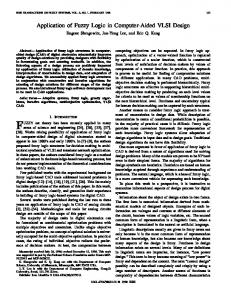
proof: Let M j = supx∈[a1 ,b1 ] f j (x). The assumptions imply that there exists w ∈ [a1 , a2 ] such that f (w) = M j for all j ∈ J. It follows that the restrictions of f j to [a1 , w] and to [w, a2 ] are non-decreasing and non-increasing, respectively. It holds that if {g i | i ∈ I} is a family of non-decreasing (non-increasing) functions, W then the function g(x) = i∈I g i (x) is non-decreasing (non-increasing). Hence, the restrictions of f to [a1 , w] and [w, a2 ] are non-decreasing and non-increasing, W respectively. It follows that f = i∈J f j is unimodal. 2 Remark 3.17 (i) We can distinguish three types of unimodal functions, which in the literature are usually denoted by Z, S and Π (see Figure 3.2 and Definition 3.18) where S denotes non-decreasing unimodal functions, Z nonincreasing unimodal functions, and Π functions which could be divided to non-decreasing and non-increasing parts. We can introduce a relation uni on the set Cu of all unimodal functions. Two functions f1 and f2 are in relation uni if they possess the same type of unimodality (one of Z, S, Π). It is easy to see that the relation uni is an equivalence. (ii) There is also another classification of unimodal functions, which will be used in Chapter 6. Due to this classification, two unimodal functions are in the same class if the intervals in which they attain its maximal values have nonempty intersection. Definition 3.18 (i) Unimodal function f is of type 1. Z if a1 = c1 = d1 and c2 6= b1 . 2. S if b1 = c2 = d2 and c1 6= a1 . 3. Π otherwise. (ii) Two unimodal functions f 1 and f 2 are in relation uni iff they both possess the same type of unimodality (one of Z, S or Π). (iii) Two unimodal functions f 1 , f 2 : [a1 , b1 ] −→ [a2 , b2 ] are in relation unim iff W there exists x0 ∈ [a1 , b1 ] such that f 1 (x0 ) = x∈[a1 ,b1 ] f 1 (x) and f 2 (x0 ) = W = x∈[a1 ,b1 ] f 2 (x). 40

b2 Z

Π

S

a2 a1

b1 Figure 3.2: Three types of unimodal functions.

Lemma 3.19 (i) Any unimodal function f has just one type of unimodality. (ii) The relation uni is an equivalence relation. (iii) The relation unim is reflexive and symmetric.

proof: Immediate.

2

Remark 3.20 It is easy to see that the relation unim is not, in general, a transitive one. Hence, it is a tolerance relation (see Section 3.4.1 and [32]). It follows that the maximal blocks of the relation unim (i.e. maximal subsets U of Cu such that for all fi , fj ∈ U fi unim fj ) induced by this relation are not disjoint, in general. Note that if there is a family of unimodal functions {fi | i ∈ I}, where I is some index set, and for all i, j ∈ I it holds that fi unim fj , then Lemma 3.16 applies to this family and W the function i∈J fi is an unimodal one. We will use this fact in Chapter 6. The next lemma shows a condition under which both relations uni and unim coincide. Lemma 3.21 Let U = {f i | i ∈ I}, U ⊆ Cu be a family of unimodal functions, f i : [a1 , b1 ] −→ [a2 , b2 ] for all i ∈ I. Denote by M fi the value supx∈[a1 ,b1 ] f i (x). Let the following conditions hold:

41

(i) There exist x0 ∈ [a1 , b1 ] and M ∈ [a2 , b2 ] such that for all functions {f j | j ∈ J} of type Π from U, J ⊆ I, it holds that f j (x0 ) = M fj = M . (ii) (f i unim f j ) implies (f i uni f j ) for all i, j ∈ I. Then the relations uni and unim coincide.

proof: We have to show that (f i uni f j ) implies (f i unim f j )

(3.18)

For two unimodal functions f1 and f2 of type Z or S, (3.18) follows from the fact that there is always x0 = a1 (or x0 = b1 ) such that f1 (x0 ) = f2 (x0 ) = M1 = M2 . For two unimodal functions of type Π, the existence of such x0 follows directly from assumption (i). 2 The following lemma will be used in the proof of Theorem 6.22, Section 6.3. Lemma 3.22 Let f 1 and f 2 be two unimodal functions from [a1 , b1 ] to [a2 , b2 ] satisfying (i)

W x∈[a1 ,b1 ]

f 1 (x) =

W x∈[a1 ,b1 ]

f 2 (x),

(ii) f 1 and f 2 are not in the relation unim . Then a function f (x) = f 1 (x) ∨ f 2 (x) is not unimodal. W f 1 (x) = x∈[a1 ,b1 ] f 2 (x). Suppose that f 1 (x1 ) = f 2 (x2 ) = M . Because f 1 and f are not in the relation unim , we know that either x1 < x2 or x1 > x2 . Suppose x1 < x2 . Then it follows from the continuity of functions f 1 and f 2 that there exists x0 such that x1 < x0 < x2 and f 1 (x0 ) < M as well as f 2 (x0 ) < M . It follows that f (x0 ) = f 1 (x0 ) ∨ f 2 (x0 ) < M . Because f (x1 ) = f (x2 ) = M , it follows that the function f (x) = f 1 (x) ∨ f 2 (x) is not unimodal. The case x1 > x2 can be proved similarly. 2

proof: Denote by M the value M =

W

x∈[a1 ,b1 ] 2

Remark 3.23 In the following text we will need to extend the notion of unimodal functions in such a way that it includes also (non-continuous) intervals, i.e. functions ( e1 , x ∈ [c1 , c2 ], f (x) = e2 otherwise 42

where e1 > e2 . If c1 = c2 , then this interval degenerates to a single point. Definitions of the relations uni and unim are identical for this wider class of unimodal functions and it can be demonstrated that all lemmas in this section also hold, so we will not explicitly distinguish between these two classes in further explanation.

43

Chapter 4 Theories for Modeling of the Meaning of Evaluating Linguistic Expressions Let us remind that in the following, we say that a structure V is a model of the theory T if it holds that SAxT (A) ≤ V(A) for all A ∈ FJ(T ) . We call a structure V a possible world for the theory T if it is a model of T and its support is a real interval [v l , v r ] (or, in case of many-sorted languages, intervals [v l1 , v r1 ], . . . , [v ln , v rn ]). Moreover, membership functions – interpretations of predicate symbols from J(T ) are continuous with respect to the standard metric on reals.

4.1

Definition of theory T ev

In this section we state several natural requirements which a logical theory aimed at a characterization of the meaning of linguistic expressions should fulfil. We are not going to define one (“unique”, “best”) theory, but postulate several axioms which all such theories should obey. We work on a lower level of abstraction than in [21]. We suppose that the members of the set S of simple evaluating expressions are translated into our formal system by means of unary predicate symbols, i.e. we have no counterpart of linguistic hedges in our language. However, even if we consider also some formalization of hedges (by unary connectives), it is possible to transform it into the system presented here, and to study its properties (e.g. if the proposed interpretation of linguistic hedges on syntactic level is done in such a way that it 44

guarantees correct behavior of the overall formal system with respect to deduction) and to compare it with other ones. We denote a fuzzy theory aimed at a characterization of simple evaluating expressions by T ev and its first-order language by J(T ev ). The (finite) nonempty set of simple evaluating linguistic expressions is denoted by S. The corresponding set of unary predicate symbols in the language J(T ev ) is denoted by G. We denote by m : S −→ G a bijection between S and G which assigns to every simple evaluating expression A ∈ S the unary predicate m(A) ∈ G. The set of all closed terms of J(T ev ) is denoted by M . In Definition 3.12, an intension of linguistic expression has been generally defined as a set of (instances of) evaluated formulas. In the following, we use provability degrees in certain formal theory T as the evaluations of instances of formulas. The intension of simple evaluating expression A ∈ S in a theory T is then n o ± ˜ G (t) Gx [t] | G = m(A), t ∈ M, T `α˜ G (t) Gx [t] Int(A) = A = α (4.1) where α ˜ G : M −→ L is a function called an intensional mapping. Note that α ˜ G (t) depends also on the theory T we are working in. Because G is a set of unary predicate symbols, for every nonempty subset {Gi | i ∈ I} ⊆ G holds that the n o ± ˜ Gi (t) Gi,x [t] | i ∈ I, t ∈ M is a set of independent evaluated formulas in the set α sense of Definition 3.6. Definition 4.1 The fuzzy theory T ev with the set of unary predicate symbols G, G ⊂ J(T ev ) is called a theory of evaluating expressions if it fulfills the following conditions: 1. The language J (T ev ) contains a set of constants large enough for the representation of real numbers, e.g. let the set of constant symbols M (which is simultaneously also the set of closed terms, provided that there are no function © ª symbols in J(T ev ) be M = t(z) | z ∈ [0, 1] . 2. For every formula G(x), G ∈ G, there exist closed terms t1 , t2 ∈ M such that T ev ` Gx [t1 ] and T ev `0 Gx [t2 ]. 3. Let γG : [0, 1] −→ [0, 1] be functions adjoined to functions α ˜ G by putting £ ¤ ¡ ¢ (4.2) γG (z) = v iff α ˜ G t(z) = v iff T ev `v Gx t(z) . The functions γG are continuous with respect to standard topology on R, differentiable (with the exception of at most finitely many points) and unimodal (see Definition 3.15). 45

4. For all G, G0 ∈ G, if γG = γG0 then G = G0 . 5. For every t ∈ M there is at least one G ∈ G such that T ev `c Gx [t] with c > 0. 6. T ev ` t(z1 ) 6= t(z2 ) iff z1 6= z2 . 7. T ev ` t(z1 ) ≤ t(z2 ) iff z1 ≤ z2 in the standard ordering on [0, 1]. Further, the following two axioms which ensure the existence of endpoints of linear ordering must be introduced: (i) (∃x)(∀y)(x ≤ y), (ii) (∃x0 )(∀y)(y ≤ x0 ) and crispness of ≤: (∀x)(∀y)(x ≤ y) ∨ ¬ (x ≤ y)

(4.3)

(∀x)(∀y)(x = y) ∨ ¬ (x = y).

(4.4)

and =: Lemma 4.2 There exists a consistent theory T ? which fulfills the requirements of Definition 4.1.

proof: Let the language of T ? be J(T ? ) = h≤, G1 , G2 , {t(z) | z ∈ [0, 1]}i where ≤ is binary predicate symbol, G1 and G2 are unary predicate symbols. Let the set of special axioms of the theory T ? be n o n o ± ± ˜ G1 (t) G1,x [t] | t ∈ M ∪ α ˜ G2 (t) G2,x [t] | t ∈ M ∪ SAxT ? = α © ± ª © ± ª ∪ 1 t(z1 ) < t(z2 ) | z1 < z2 , z1 , z2 ∈ [0, 1] ∪ 1 (∃x)(∀y)(x ≤ y) © ± ª © ± ª ∪ 1 (∃x0 )(∀y)(y ≤ x0 ) ∪ 1 (∀x)(∀y)(x ≤ y) ∨ ¬ (x ≤ y) © ± ª ∪ 1 (∀x)(∀y)(x = y) ∨ ¬ (x = y) (4.5) ¢ ¢ ¡ ¡ where t(z1 ) < t(z2 ) is an abbreviation for t(z1 ) ≤ t(z2 ) & t(z1 ) 6= t(z2 ) . Let the functions α ˜ G1 and α ˜ G2 be ¡ ¢ 4 α ˜ G1 t(z) = (1 − z) ∨ 0, 3

¡ ¢ 1 4 α ˜ G2 t(z) = (− + z) ∨ 0. 3 3

ˆ 1, G ˆ 2 i where ≤ is the standard ordering Let us define a structure M = h[0, 1], ≤, G ¡ ¢ ˆ 1, G ˆ 2 are unary fuzzy relations defined by G ˆ 1 (x) = α of real numbers, G ˜ G1 t(x) and 46

¡ ¢ ˆ 2 (x) = α G ˜ G2 t(x) . The interpretation of constant symbols from J(T ? ) is defined ¡ ¢ by M t(z) = z, z ∈ [0, 1]. It is easy to see that M is a model of T ? , hence T ? is consistent. We show that T ? fulfills the requirements of Definition 4.1. Item 1 of Definition 4.1 is fulfilled due to the definition of J(T ? ), for item 2 consider terms t(0) and £ ¤ ± £ ¤ t(1) for G1 : T ? ` G1,x t(0) because there is a special axiom of the form 1 G1,x t(0) ¡ £ ¤¢ £ ¤ in SAxT ? . Because M G1,x t(1) = 0, it follows that T ? `0 G1,x t(1) . Analo£ ¤ £ ¤ gously, T ? ` G2,x t(1) and T ? `0 G2,x t(0) . Items 3, 4, 6 and 7 are straightfor© ª ward, for item 5 consider the set M1 = t(z) | z ∈ [0, 0.6] , for which it holds that © ª T ? `ct G1,x [t], t ∈ M1 , ct > 0, and analogously M2 = t(z) | z ∈ [0.4, 1] , for which it holds that T ? `ct G2,x [t], t ∈ M2 , ct > 0. It follows that for all t ∈ M , T ? `ct Gx [t] for some G ∈ G and with ct > 0. 2 Remark 4.3 (i) In the previous definition we index the members of the set M of closed terms either by subscripts (e.g. t1 , t2 ) where subscripts mean the usual indexing via some fixed index set, or by superscripts (e.g. t(z) , z ∈ [0, 1]), by which we denote (unique) closed term corresponding to the real number z. We will keep this notation throughout the rest of the thesis. (ii) Item 2 of the previous definition articulates the requirement that the properties expressed by simple evaluating expressions should be completely valid for some objects and completely invalid for the other ones. Item 3 expresses the fact that vagueness cannot change abruptly (it is continuous). Item 4 requires that the adjoined functions γG should be pairwise different. The reason is that the predicate symbols G are formalizations of different evaluating linguistic expressions and it is counterintuitive to assign the same meaning to different expressions. Item 5 states that every abstract object t(z) corresponding to the real number z from [0, 1] has some property in a non-zero degree, i.e. that the set S of simple evaluating expressions is rich enough in the sense that there are no “gaps” for which no properties are described by the theory T ev . Finally, Item 7 ensures us that the set M of closed terms is linearly ordered in the same way as interval [0, 1] and this ordering has endpoints. (iii) The intensional mappings of the atomic formulas G(x) ∈ G can be computed inside some other theory, e.g. the theory of evaluating syntagms T EV described in [21]. Formulas which correspond to simple evaluating expressions are there composed from predicate symbol for horizon L, members of a set of unary 47

connectives ¢ α representing linguistic hedges, and function symbol η for order-reversing automorphism. It means that these formulas are not independent, in general. (iv) The intended semantics of the theory T ev is as follows: the support of such a structure is a real interval, predicate symbols G ∈ G are interpreted as unary fuzzy relations (fuzzy subsets) of D. Object constants t(z) are interpreted by ¡ ¢ ¡ ¢ real numbers z ∈ D in such a way that if z1 < z2 then D t(z1 ) < D t(z2 ) . (v) We require in Item 3 that functions γG (z), z ∈ [0, 1] have to be unimodal. Because unimodal functions could be divided to several categories by means ev of the relations uni and unim (see Remark 3.17), we can define relations uniT ev and uniTm on the set Shxi of intensions of simple evaluating expressions (for formal definitions see Definition 4.4). Two intensions A1,hxi and A2,hxi are in ev relation uniT iff for the functions γAi associated to their intensional mappings ev α ˜ Ai hold that γA1 uni γA2 , and similarly is defined the relation uniTm . Note that these relations are dependent on the assignment of intentions Ai,hxi to evaluating linguistic expressions Ai ∈ S and consequently on theory T ev . It is ev ev easy to see that the relations uniT and uniTm are equivalence and tolerance ev relations, respectively. Therefore, the relation uniT induce a partition on the set Shxi . In accordance with the discussion presented in Section 3.2, we prefer to use three atomic evaluating expressions small, medium and big in such a way that their intensional mappings belong to classes Z, Π and S, respectively. In this case the intensions Ahxi ∈ Shxi of simple evaluating expressions are divided ev ev by relations uniT and uniTm into three disjoint subsets and both relations coincide (due to Lemma 3.21). We can also include into the definition of the theory T ev the requirement, that if two linguistic expressions A1 and A2 have the same atomic expression, then their respective intensions A1,hxi and A2,hxi T ev should be in the relation unim . Definition 4.4 Denote by Shxi a set of intensions of simple evaluating linguistic expressions (with respect to a given theory T ev ), i.e. © ª Shxi = Ahxi | A = m(A) and A ∈ S ± ˜ A (t) Ax [t] | t ∈ M }. A relation uniT ev ⊆ Shxi × Shxi is defined by where Ahxi = {α means of the intensional mappings α ˜A: ev

(A1,hxi uniT A2,hxi ) iff (γA1 uni γA2 ) 48

where the functions γAi , i = 1, 2 are defined by (4.2) and the relation uni is defined ev in Definition 3.18. Analogously is defined a relation uniTm ⊆ Shxi × Shxi : ev

(A1,hxi uniTm A2,hxi ) iff (γA1 unim γA2 ). Lemma 4.5 For any theory of evaluating expressions T ev it holds that: (i) The relation uniT

ev

is an equivalence relation.

T ev

(ii) The relation unim is a tolerance relation.

proof: Item 3 of Definition 4.1 requires that the functions α˜ A should be unimodal for any theory of linguistic description T ev . The claims then follow from Definition 3.18 of relations uni and unim . 2

4.2

Canonical possible worlds

Definition 4.6 A canonical possible world VC of the theory of evaluating expressions T ev is a model ¡ ¢ VC = h[0, 1], . . .i of T ev such that VC t(z) = z for z ∈ [0, 1], for which the following property holds for all G ∈ G and t ∈ M : VC (Gx [t]) = α ˜ G (t).

(4.6)

The question of existence of such a canonical possible world is addressed by the following theorem. Theorem 4.7 Let a theory T fulfil the conditions of Definition 4.1. Suppose that the fuzzy set of special axioms of the theory T has the following property (C): For every formula B, every atomic formula Gx [t], G ∈ G, t ∈ M and every truth valuation W : FJ(T ) −→ L it holds that: If Gx [t] is a subformula of B and SAx(Gx [t]) ≤ W(Gx [t]) then SAx(B) ≤ W(B). Then there exists canonical possible world VC |= T in the sense of Definition 4.6.

49

proof: Due to item 2 of Definition 4.1, the theory T is consistent (because there exists some formula with provability degree equal to 0), hence it has a model. From item 6 of Definition 4.1 and L¨owenheim-Skolem Theorem (cf. Theorem 4.35, [27]) it follows that there exists a model U of T of cardinality of continuum. From Item 7 of Definition 4.1 follows that the support of U is linearly ordered and this ordering has endpoints. Consider a structure V with the support V = [0, 1] and an order-preserving bijection g : U −→ V . Let the interpretation of constants in V be defined by V(t) = g(U(t)), of function symbols by V(f (t1 , . . . , tn )) = g(U(f (t1 , . . . , tn ))) and interpretation of predicate symbols by V(P (t1 , . . . , tn )) = U(P (t1 , . . . , tn )). It follows that V is a model of T . Now we can construct a structure VC from V which differs only in the evaluations of Gx [t] defined by VC (Gx [t]) = α ˜ G (t). It is possible because Gx [t] are closed instances of atomic predicate formulas. We show that VC is a model of T . If B contains no subformula of the form Gx [t] then VC (B) = V(B) ≥ SAx(B). Otherwise, SAx(B) ≤ VC (B) by assumption (C). It follows that VC is a canonical possible world for T . 2 Remark 4.8 A theory T which fulfills property (C) will be called simple. For simple theories of evaluating expressions, canonical possible worlds always exist. The existence of canonical possible worlds is important, because it guarantees the existence of possible worlds where membership functions of fuzzy sets, which are interpretations of predicate symbols G ∈ G, have the properties required in Definition 4.1.

4.3

Extended theories

Canonical possible worlds from Definition 4.6 can be understood as models in which truth functions mimic the behavior of intensional mappings of predicate symbols G ∈ G from the theory T ev . In the following we define a wider class of models in which the interpretations of predicate symbols G ∈ G behave “similarly” as in the canonical possible world V, but these interpretations are restricted also from above. To this purpose we extend (some fixed) fuzzy theory T ev by axioms on negations of (instances of) predicate symbols G ∈ G and we also require continuity and unimodality of membership functions of their interpretations in appropriate models. 50

Definition 4.9 An extended theory of evaluating expressions T evx arises from the theory T ev by expanding it by axioms n o ± β˜G (t) ¬ Gx [t] | G ∈ G, t ∈ M (4.7) where β˜G (t) : M −→ L and α ˜ G (t) ⊗ β˜G (t) = 0

(4.8)

holds for all t ∈ M . Remark 4.10 (i) The requirement (4.8) is equivalent to β˜G (t) ≤ ¬˜ αG (t) for all ˜ t ∈ M and also to α ˜ G (t) ≤ ¬βG (t) for all t ∈ M . (ii) We can unify the notation by denoting both sets of evaluated formulas (i.e. instances of formulas Ax [t] and ¬ Ax [t]) by one symbol Ae , i.e. n o n o ± ± ˜ e α ˜ (t) β (t) ¬ A A := Ax [t] | t ∈ M ∪ A Ax [t] | t ∈ M , (4.9) provided that (4.8) holds for all t ∈ M . (iii) The values ¬˜ αG (t) are consistency thresholds for the formulas Gx [t] in the sense of Definition 1 from [26]. There is also some relation to the concept of intuitionistic fuzzy sets introduced by K. Atanasov. Lemma 4.11 If T ev is simple (see Remark 4.8), then T evx is consistent and T evx `d ¬ Gx [t] where d = β˜G (t), for all G ∈ G and t ∈ T .

proof: The canonical possible world VC of T ev from Definition 4.6 is also a ¬Gx [t]) = ¬VC (Gx [t]) = ¬˜ ¬Gx [t]) model of T evx , because VC (¬ αG (t) ≥ β˜G (t) = SAx(¬ evx holds. Therefore, T is consistent. For the second part of lemma, it is sufficient ¬Gx [t]) = β˜G (t), which can be done by to construct such a model U for which U(¬ the same technique as in the proof of Theorem 4.7. The claim then follows from the Completeness Theorem. 2 Definition 4.12 An extended possible world of T evx is a model VE of the extended theory of evaluating expressions such that its support is a closed interval [a, b] ⊂ R, interpretation of ¡ ¢ closed terms is VE t(z) = a + (b − a)z, z ∈ [0, 1], t(z) ∈ M and interpretations of predicate symbols G ∈ G are continuous and unimodal functions GVE : [a, b] −→ L.

51

Theorem 4.13 If there exists the canonical possible world VC of T ev then there exists also the extended possible world VE of T evx and α ˜ G (t) ≤ VE (Gx [t]) ≤ ¬β˜G (t)

(4.10)

holds for all G ∈ G and all t ∈ M .

proof: The canonical possible world VC of T ev is also a model of the extended theory T evx (see the proof of Lemma 4.11). For any structure U such that U |= T evx , U(Gx [t]) ≥ SAx(Gx [t]) = α ˜ G (t). Let us prove the inequality VE (Gx [t]) ≤ ¬β˜G (t). Suppose that U(Gx [t]) > ¬β˜G (t). Then ¬Gx [t]) = ¬U(Gx [t]) < β˜G (t) = SAx(¬ ¬Gx [t]), hence U is not a model of T evx – a U(¬ contradiction. 2 Lemma 4.14 Let T evx be an extended theory of evaluating expressions such that for all G ∈ G and all t ∈ M , β˜G (t) = ¬˜ αG (t). Then all extended possible worlds VE of T evx are G-isomorphic (see Definition 3.11) with the canonical possible world VC .

proof:

It is easy to see that ³ ´ ³ ´ β˜G (t) = ¬˜ αG (t) implies α ˜ G (t) = ¬β˜G (t) .

(4.11)

From (4.6) we obtain that VC (Gx [t]) = α ˜ G (t) and from (4.10) and (4.11) it follows that α ˜ G (t) = VE (Gx [t]), i.e. VC (Gx [t]) = VE (Gx [t]). Let g : VC −→ VE be defined by g(z) = a + (b − a)z. This is a bijection between VC = [0, 1] and VE = [a, b] ⊂ R. Now we show that GVC (z) = GVE (g(z)). ¡ £ ¤¢ ¡ ¢ ¡ £ ¤¢ GVC (z) = VC Gx t(z) = α ˜ G t(z) = VE Gx t(z) = GVE (a+(b−a)z) = GVE (g(z)). Consequently, VC and VE are G-isomorphic.

2

As a generalization of this result for general extended theories we obtain the following Theorem 4.15 Let T evx be an extended theory of evaluating expressions. Then two extended possible worlds VE 1 , VE 2 of T evx are G-isomorphic in the degree greater than or equal to _ _³ ¡ (z) ¢´ ¡ (z) ¢ ˜ . (4.12) −α ˜G t c=1− ¬βG t G∈G t∈M

52

proof: Let VE i = [ai , bi ], i = 1, 2. We have to show that there exists a function g, g : VE 1 −→ VE 2 such that (i) g is a bijection between VE 1 and VE 2 , (ii) ¡ ¢ ¡ ¡ ¢¢ g VE 1 t(z) = VE 2 t(z) for all z ∈ [0, 1] and (iii) (G1i (y) ↔ G2i (g(y))) ≥ c, where Gji = VE j (Gi ), Gi ∈ G, j = 1, 2 and y ∈ VE 1 . Let g be defined as the linear transformation of VE 1 to VE 2 , i.e. for y ∈ VE 1 let g(y) = a2 +

b2 − a2 (y − a1 ). b1 − a1

Then (i) is fulfilled, (ii) ¡ ¡ ¢¢ ¡ ¢ g VE 1 t(z) = g(a1 + (b1 − a1 )z) = a2 + (b2 − a2 )z = VE 2 t(z) . (iii) Let y ∈ VE 1 , y = VE 1 (t) for some t ∈ M and let Gi ∈ G. Then from Theorem 4.13 it follows that (G1i (y) ↔ G2i (g(y))) = 1 − |G1i (y) − G2i (g(y))| ≥ 1 − (¬β˜Gi (t) − α ˜ Gi (t)), because g(y) = VE 2 (t). The claim follows from the fact that we considered general y ∈ VE 1 and Gi ∈ G, and that there is a bijection between the set of closed terms M and the set VE 1 . 2 Hence, if we put β˜G (t) = ¬˜ αG (t) for all G ∈ G and t ∈ M , then all possible worlds with the support [a, b] and natural interpretation of object constants t(z) , z ∈ [0, 1] are G-isomorphic with the canonical possible world VC . It means that possible worlds of such a theory behave in the same way as models of complete theories with respect to atomic formulas of the form Gx [t] – their provability degrees copy the structure of truth values, i.e. if T evx `α˜ G1 (t) G1,x [t] and T evx `α˜ G2 (t) G2,x [t] then T evx `c(t) G1,x [t]&¯ G2,x [t] where c(t) = α ˜ G1 (t) ¯ α ˜ G2 (t). Here &¯ is a propositional connective and ¯ is its semantic interpretation. This situation is convenient. However, it also seems to be too restrictive – all possible worlds are isomorphic and there is no freedom in choice of the interpretations of extensions of simple evaluating expressions. Now we prove (with a use of the Completeness Theorem) a lemma about lower bounds for provability degrees of propositional formulas in extended theories. In the sequel we use (A 6⇔ B) as an abbreviation for ¬ (A ⇔ B). Lemma 4.16 Let T be a consistent fuzzy theory, A and B closed formulas, T `d1 A, T `d2 B, T `e1 ¬ A and T `e2 ¬ B, and it holds that e1 ≤ ¬d1 and e2 ≤ ¬d2 , then 53

(i) T `d A ⇒ B, where d ≥ ¬e1 → d2 ,

(4.13)

T `d A ⇔ B, where d ≥ (¬e1 → d2 ) ∧ (¬e2 → d1 ),

(4.14)

T `d A 6⇔ B, where d ≥ ((d1 ⊗ e2 ) ∨ (d2 ⊗ e1)),

(4.15)

T `d A & B, where d1 ⊗ d2 ≤ d ≤ ¬e1 ⊗ ¬e2 ,

(4.16)

T `d A ∧ B, where d = d1 ∧ d2 ,

(4.17)

T `d A ∨ B, where d1 ∨ d2 ≤ d ≤ ¬e1 ∨ ¬e2 .

(4.18)

(ii)

(iii)

(iv)

(v)

(vi)

proof: (i) We use Completeness Theorem: T `d A ⇒ B implies d=

^

{D(A ⇒ B) | D |= T } =

D

≥

_

^

{D(A) → D(B) | D |= T } ≥

D

{D(A) | D |= T } →

D

^

{D(B) | D |= T } = ¬e1 → d2

D

where we have used the fact that the operation → is antitonic in the first and isotonic in the second variable. (ii) A ⇔ B := (A ⇒ B) ∧ (B ⇒ A). By the same consideration as in the previous item, T `d A ⇔ B implies d=

^

{D(A ⇔ B) | D |= T } =

D

= =

^

^

^

{D(A) ↔ D(B) | D |= T } =

D

{(D(A) → D(B)) ∧ (D(B) → D(A)) | D |= T } =

D

{(D(A) → D(B)) | D |= T } ∧

D

^

{(D(B) → D(A)) | D |= T } ≥

D

≥ (¬e1 → d2 ) ∧ (¬e2 → d1 ).

54

(iii) d= = =1−

_

^

^

{D(A 6⇔ B) | D |= T } =

D

{1 − D(A ⇔ B) | D |= T } =

^

D

^

¬(A ⇔ B)) | D |= T } = {(D(¬

D

{1 − (D(A) ↔ D(B)) | D |= T } =

D

{D(A) ↔ D(B) | D |= T } = 1 −

D

_

{1 − |D(A) − D(B)| | D |= T } =

D

=

^

{|D(A) − D(B)| | D |= T }.

D

It can be easily seen that the expression on the last line attains minimal value at the point à ! _ ^ {D(A) | D |= T } − {D(B) | D |= T } ∨ D à D ! ^ _ ∨ {D(B) | D |= T } − {D(A) | D |= T } ∨ 0. D

D

And this expression is equal to ((d1 − ¬e2 ) ∨ (d2 − ¬e1)) ∨ 0 which could be written, using the definition of L Ã ukasiewicz conjunction, as ((d1 ⊗ e2 ) ∨ (d2 ⊗ e1)). (iv) The fact that d1 ⊗ d2 ≤ d has been proved in the item (b) of Theorem 10 of V [27]. Suppose that d > ¬e1 ⊗ ¬e2 . By the completeness, d = (D(A & B)) = D V = (D(A) ⊗ D(B)). But D(A) ≤ ¬e1 and D(B) ≤ ¬e2 , so D(A) ⊗ D(B) ≤ D V ≤ ¬e1 ⊗ ¬e2 , hence (D(A) ⊗ D(B)) ≤ ¬e1 ⊗ ¬e2 , which contradicts d > ¬e1 ⊗ ¬e2 .

D

(v) Coincides with item (d) of Theorem 10 of [27]. (vi) Analogous to the proof of item (iii). 2 Remark 4.17 Lemma 4.16 shows that in extendedn theories we can use the addio ± tional information provided by axioms of the form β˜G (t) ¬ Gx [t] | G ∈ G, t ∈ M 55

for sharper determination of the bounds of provability degrees for formulas of type G1,x [t]&¯ G2,x [t]. For example, the lower bound for the provability degree d of formula A ⇒ B in a theory T , provided that we have T `d1 A and T `d2 B, is d ≥ d2 (compare with formula (4.13)).

4.4

Theories T ev and T evx with fuzzy equality

When we use theories T ev or extended theories T evx it is advantageous to allow also the possibility to express similarity among objects. Therefore we extend the language J(T ev ) (or J(T evx )) by fuzzy equality predicate ≈ (see Section 3.1.8). Definition 4.18 A theory of evaluating expressions T≈ev is called a theory of evaluating expressions with fuzzy equality if its language contains the fuzzy equality predicate ≈ and the set of its special axioms SAx(T≈ev ) includes the axiom schemata (E1), (E2) and (E3) from Section 3.1.8 with the exponents m1 , . . . , mn equal to 1. Lemma 4.19 Let t1 , t2 ∈ M . Denote by c the value c=

_

{D(t1 ≈ t2 ) | D |= T≈ev }.

D

Then T≈ev `¬c t1 6≈ t2 .

proof: From the Completeness Theorem (cf. Theorem 3.5) it follows that T≈ev `d t1 6≈ t2 , where d= =

^

^

{D(t1 6≈ t2 ) | D |= T≈ev } =

^

{¬D(t1 ≈ t2 ) | D |= T≈ev } =

D

D

{1 − D(t1 ≈ t2 ) | D |= T≈ev } = 1 −

D

=¬

_

_

{D(t1 ≈ t2 ) | D |= T≈ev } =

D

{D(t1 ≈ t2 ) | D |= T≈ev } = ¬c.

D

2 56

Chapter 5 Linguistic Descriptions This section presents the treatment of linguistic descriptions on linguistic, syntactic and semantic levels.

5.1

Linguistic level

On the linguistic level, a linguistic description is a set of linguistic expressions of the form “IF A THEN B”, where A and B are evaluating linguistic predications (cf. Section 3.2.1). Definition 5.1 A linguistic description in FLb is a finite set LDI = {RI1 , RI2 , . . . , RIr } of conditional clauses RIi := IF Ai THEN Bi , i = 1, 2, . . . , r (5.1) where Ai , Bi are evaluating predications. If all evaluating predications Ai , Bi are simple (cf. Section 3.2.2) then also the linguistic description LDI is called simple. Remark 5.2 (i) By An(Ri ) we denote the antecedent part of the rule Ri , i.e. An(Ri ) = Ai , and, similarly for the succedent part, Succ(Ri ) = Bi . An(LDI ) denotes the set of all antecedents and Succ(LDI ) the set of all consequents of the linguistic description LDI , i.e. An(LDI ) = {Ai | i = 1, 2, . . . , r} and Succ(LDI ) = {Bi | i = 1, 2, . . . , r}. (ii) It is possible to consider also IF-THEN rules which include negations too, e.g. 1 RIn := IF Ai THEN NOT Bi , i

57

(5.2)

5.2

2 RIn := IF NOT Ai THEN Bi , i

(5.3)

3 RIn := IF NOT Ai THEN NOT Bi . i

(5.4)

Level of syntax

The intensions of individual conditional clauses RIi are determined by the theories of evaluating expressions T1ev and T2ev for antecedent and consequent parts of IF-THEN rules, respectively. The theories T1ev and T2ev could be identical, but it is usually advantageous to use different theories for antecedents and for consequents. The language in which the intension of IF-THEN rule is written down is the two-sorted first-order language © ª © ª J(TI ) = hG1 , G2 , t(z) | z ∈ [0, 1] , s(z) | z ∈ [0, 1] , . . .i where Gi , i = 1, 2 is the set of atomic predicate symbols for sort i, discussed in the Section 4.1. The set of all closed terms of the sort i are denoted by Mi . The intension of one IF-THEN rule is constructed from the intensions of its antecedent part n o ± ˜ Ai (t) Ai,x [t] | t ∈ M1 Ai,hxi = α (5.5) and its succedent part n

Bi,hyi

o ± α ˜ (s) Bi = Bi,y [s] | s ∈ M2

(5.6)

in the following way: Ri,hx,yi = Ai,hxi ⇒ Bi,hyi = n o ± α ˜ (t, s) ⇒ A ⇒ B = Ai,x [t] Bi,y [s] | t ∈ M1 , s ∈ M2 , Ai ∈ G1 , Bi ∈ G2 . i i (5.7) In the sequent by Ai , Bi we denote the formulas from (5.5) and (5.6) respectively, i.e. the formulas the instances of which are used in construction of the intension of i-th IF-THEN rule in the linguistic description LDI . The syntactic evaluations α ˜ Ai⇒ Bi should by constructed by means of syntactic evaluations of Ai and Bi , respectively. This means that ¬β˜Ai (t) → α ˜ Bi (s) ≤ α ˜ Ai⇒ Bi (t, s) ≤ α ˜ Ai (t) → ¬β˜Bi (s)

58

(5.8)

should hold (in case that T1ev or T2ev are not extended theories of evaluating expressions, β˜A (t) are equal to 0.) It can be easily shown that the inequality ˜ Bi (s) ≤ α ˜ Ai (t) → ¬β˜Bi (s) ¬β˜Ai (t) → α from (5.8) always holds, provided that α ˜ Ai (t) ≤ ¬β˜Ai (t) and α ˜ Bi (s) ≤ ¬β˜Bi (s), which follows from Definition 4.9. Remark 5.3 The question which arises now is how to determine the intensional mapping α ˜ Ai⇒ Bi (t, s). The most natural possibility, which is also in accordance with Frege principle of compositionality (saying that the intension of a compound expression is a function of intensions of its parts), is to put α ˜ Ai⇒ Bi (t, s) = α ˜ Ai (t) → α ˜ Bi (s).

(5.9)

Intension of the conditional clause IF A THEN B is defined in this way in [27], Definition 6.10, p. 238. However, it is not necessary to suppose this in the proof of Theorem 6.5 of this thesis. A linguistic description LDI naturally leads to the theory of linguistic description TI in the language J(TI ) if we construct its fuzzy set of special axioms from the intensions Ri,hx,yi , i.e. we put © ª TI = Ri,hx,yi | i = 1, 2, . . . , r .

(5.10)

Remark 5.4 If we work with extended theories of evaluating expressions T evx (see Section 4.3), and there are IF-THEN rules (given by expert or extracted by some algorithm) which include negations, then it is possible (and advantageous) to ex¯ hxi , B ¯ hyi the tend also the theory TI by corresponding axioms. Let us denote by A multiformulas o n ± ¯ hxi = β˜A (t) ¬ Ax [t] | t ∈ M1 , A (5.11) o n ± ¯ hyi = β˜B (s) ¬ By [s] | s ∈ M2 , (5.12) B ¯ hxi is the mapping β˜A (t) respectively, i.e. the intensional mapping of multiformula A from Definition 4.9. If there are IF-THEN rules RIj := IF Aj THEN NOT Bj , j ∈ 1, 2, . . . , r,

(5.13)

RIk := IF NOT Ak THEN NOT Bk , k ∈ 1, 2, . . . , r,

(5.14)

59

RIl := IF NOT Al THEN Bl , l ∈ 1, 2, . . . , r,

(5.15)

¯ j,hyi , A ¯ k,hxi ⇒ B ¯ k,hyi and then we can construct the multiformulas Aj,hxi ⇒ B ¯ l,hxi ⇒ Bl,hyi , respectively, with their intensional mappings computed via the comA positionality principle, i.e. o n ± ˜ ¯ (s) α ˜ (t) → β Ai Bi Ai,x [t] ⇒ ¬ Bi,y [s] | t ∈ M1 , s ∈ M2 , (5.16) Ai,hxi ⇒ Bi,hyi = n o ± ¯ i,hxi ⇒ B ¯ i,hyi = β˜Ai (t) → β˜Bi (s) ¬ Ai,x [t] ⇒ ¬ Bi,y [s] | t ∈ M1 , s ∈ M2 , (5.17) A n o ± ¯ i,hxi ⇒ Bi,hyi = β˜Ai (t) → α ˜ Bi (s) ¬ Ai,x [t] ⇒ Bi,y [s] | t ∈ M1 , s ∈ M2 . (5.18) A We will denote this theory by TIE ; note that if the original theories T ev are not extended ones, we put β˜Ai (t) = 0 for all i = 1, . . . , r and t ∈ M1 and, similarly, β˜Bi (s) = 0 for all i = 1, . . . , r and s ∈ M2 . Then, we put ¯ i,hyi , A ¯ i,hxi ⇒ B ¯ i,hyi , A ¯ i,hxi ⇒ Bi,hyi }. TIE = {Ai,hxi ⇒ Bi,hyi , Ai,hxi ⇒ B

Remark 5.5

(5.19)

(i) Let us consider the following form of IF-THEN rule (5.2), namely RIj := IF A THEN NOT B

where B is a simple evaluating predication. Then, the interval of admissible syntactic evaluations of a formula Ax [t] ⇒ ¬ By [s] is ¬β˜A (t) → β˜B (s) ≤ α ˜ A⇒ ˜ A (t) → ¬˜ αB (s). ⇒¬ B (t, s) ≤ α

(5.20)

(ii) In the sequel we will need to work with antecedent and consequent parts of the linguistic description LDI on the level of syntax. The following theories are introduced: TIA = {Int(An(Ri )) | i = 1, 2, . . . , r} = {Ai | i = 1, 2, . . . , r}

(5.21)

TIS = {Int(Succ(Ri )) | i = 1, 2, . . . , r} = {Bi | i = 1, 2, . . . , r}.

(5.22)

and

For extended theories in the sense of Definition 4.9 the theories TIA and TIS ± are also extended by the axioms {β˜Ai (t) ¬ Ai,x [t] | t ∈ M1 , i ∈ 1, 2, . . . , r} and ± {β˜Bi (s) ¬ Bi,y [s] | s ∈ M2 }, respectively. 60

5.3

Level of semantics

On the semantic level, given a possible world V = hhV1 , V2 i, {Ai | i ∈ {1, . . . , r}}, {Bi | i ∈ {1, . . . , r}}, . . .i where Ai , Bi are fuzzy sets – interpretations of atomic predicate symbols Ai ∈ G1 , Bi ∈ G2 , each fuzzy IF-THEN rule Ri ∈ LDI is assigned an extension in V: ¯ o n ± ¯ (5.23) ExtV (Ri ) = V(Ai,x [u] ⇒ Bi,y [v]) hu, vi¯ hu, vi ∈ V1 × V2 . Note that the extension of the rule Ri is a fuzzy relation ExtV (Ri ) = R ⊂ V1 × V2 . ∼ Theorem 5.6 Let LDI be a linguistic description and (5.9) hold. Then the theory TI is consistent and there exists possible world W = hhW1 , W2 i, {Ai | i ∈ {1, . . . , r}}, {Bi | i ∈ {1, . . . , r}}, . . .i such that W(Ai,x [t] ⇒ Bi,y [s]) = α ˜ Ai⇒ Bi (t, s).

proof: Let us construct the model W: define Wj = [0, 1], j = 1, 2 and ¡ ¢ ¡ ¢ Ai (x) = α ˜ Ai t(x) for x = W t(x) , t(x) ∈ M1 and x ∈ [0, 1]. Analogously, ¡ ¢ ¡ ¢ Bi (y) = α ˜ Bi s(y) for y = W s(y) , s(y) ∈ M2 and y ∈ [0, 1]. Then

W(Ai,x [t] ⇒ Bi,y [s]) = W(Ai,x [t]) → W(Bi,y [s]) = Ai (W(t)) → Bi (W(s)) = =α ˜ Ai (t) → α ˜ Bi (s) = α ˜ Ai⇒ Bi (t, s). It follows that W |= TI and, therefore, TI is a consistent theory.

2

Possible worlds isomorphic to the possible world W from the proof of Theorem 5.6 will be called canonical possible worlds for TI .

61

Chapter 6 Fuzzy Logic Deduction In this chapter we present basic scheme of fuzzy logic deduction and analyze the concept of inconsistency of linguistic description. We present two different definitions of inconsistency. Let us stress that this inconsistency is not considered in the strict logical sense, but rather from the point of view of applications of a linguistic description in concern.

6.1

Basic scheme

The basic scheme of fuzzy logic deduction is the following: We have at our disposal the fuzzy theory TI (5.10) composed of implications and a fuzzy theory T 0 which represents an observation. From these theories we form a theory TD = TI ∪ T 0 . The theory TI expresses the relationship between antecedent and succedent variables. The problem (addressed in Chapter 7) is how an observation u0 measured in some possible world V can be transformed into its logical counterpart T 0 . The general form of T 0 is © ª T 0 = A0i,hxi | i ∈ I (6.1) where I ⊆ {1, 2, . . . , r} and A0i,hxi =

n

o ± 0 α ˜A (t) A [t] | A = m(A ) . i,x i i i

(6.2)

Definition 6.1 Let a theory TD = TI ∪ T 0 be consistent. Then the conclusion is defined by B0 = {B0i,hyi | i ∈ K} 62

(6.3)

where

n o ± 0 ˜B (s) B0i,hyi = α B [s] | s ∈ M i,y 2 , i

(6.4)

0 and α ˜B (s) = c iff TD `c Bi,y [s]. i

Generally, a theory T 0 can contain several intensions A0i , and then also the conclusion B0 is composed of several parts. Remark 6.2 (i) Note that formulas Ai,x [t] appear in the intensions of antecedent part of individual IF-THEN rules in the theory TI and also in the intensions 0 (6.2). But, their syntactic evaluations, i.e. the functions α ˜ Ai (t) and α ˜A (t) can i be (and usually are) different. (ii) Index sets I and K are not identical, in general. They have the same cardinality in case there do not exist two IF-THEN rules with identical antecedent and different succedent parts in the linguistic description LDI . Otherwise, if the theory TI contains intensions Ri,hx,yi = Ai,hxi ⇒ Bi,hyi and Rj,hx,yi = Aj,hxi ⇒ Bj,hyi where Ai = Aj and Bi 6= Bj and o © ª n 0 ± ˜ Ai (t) Ai,x [t] | t ∈ M1 T 0 = A0i,hxi = α which means that I = {i}, then both intensions Ri,hx,yi and Rj,hx,yi are used in deduction and the conclusion B0 will be B0 = {B0i,hyi | i ∈ K} where K = {i, j} 6= I. Of course, linguistic descriptions with such rules are in some sense incorrect or “inconsistent”, we will study such descriptions and problems connected with them in Section 6.2. (iii) Formula (6.2) also means that we can use only intensions contained in some of antecedent parts of IF-THEN rules in a linguistic description LDI , when we are translating the observation (obtained on semantic level) into the level of formal syntax. Hence, even if there is some linguistic expression A ∈ S and corresponding unary predicate A = m(A) ∈ G which would be best for the description of the observation, it could not be used unless there is a rule Ri := IF X IS A THEN Y IS B in LDI . 63

(iv) Note that our basic scheme implies that the following basic principle of (logical) deduction is kept: The deduction is performed only when there is enough evidence for doing it. This means in our case that the deduction gives some result only if there is the same formula Ai in the intension of some rule Ri from LDI , and in A0i,hxi . If it is not the case (for example consider IF-THEN rules with antecedents A1 = small and A2 = big, and the observation is e.g. about 0.5 ) then it happens that the conclusion B0 is empty. The theory T 0 usually represents a single observation. The observation can be a crisp number or linguistic expression, which expresses precisely or vaguely the position on an ordered scale. Therefore, the theory T 0 cannot be completely arbitrary and should fulfil some requirements. We can distinguish two situations — the index set I has cardinality equal to one, which means that the observation is translated into one multiformula. This is possible in situations when there is one rule Ri in LDI whose antecedent fits the observation better than antecedents of other IF-THEN rules. If there is no such rule, then it is necessary to use several rules {Ri | i ∈ I}, but the theory T 0 should still reflect the fact that it represents single observation. We will formulate this requirement in the following definition. Definition 6.3 We say that a theory

© ª T 0 = A0i,hxi | i ∈ I

represents a single observation, if 0 0 0 0 1. all functions α ˜A are identical, i.e. α ˜A = α ˜A = ··· = α ˜A = α ˜ 0 where i i1 i2 in i1 , i2 , . . . , in ∈ I.

2. The function γ adjoined to the function α ˜ 0 in the same way as in formula (4.2) is either (a) continuous, unimodal and there are z1 , z2 ∈ [0, 1] such that γ(z1 ) = 1 and γ(z2 ) = 0, or (b) γ(z) = 1 for z ∈ [zl , zr ] and γ(z) = 0 otherwise. Remark 6.4 Let us explain the intuition behind the previous definition. The de0 grees α ˜A (t) express the truth of the proposition “Object named t characterizes i the observed quantity.” Therefore it should not depend on the (atomic) formula Ai (Item 1 of the definition.) 64

If we accept the principle saying that the vagueness can change only continuously, 0 then it is natural to require that the function γ adjoined to functions α ˜A should i be continuous. If it would not be unimodal, then it can hardly represent single observation, having e.g. two local maxima. We should also exclude too non-specific representations like α ˜ 0 (t) = 1 for all t, which are, strictly speaking, unimodal, but do not characterize any value. On the other hand, there is a natural non-continuous characterization of a single value, namely singleton or interval (Item 2b). The fact that the following theorem holds is crucial for the applicability of fuzzy 0 logic deduction. It enables us to compute intensional mappings α ˜B of the conclusion. i It is also in accordance with the classical formula obtained on the level of semantics by standard manipulations with fuzzy relations. Theorem 6.5 Let LDI be a simple linguistic description and the theory TD = TI ∪T 0 be constructed as above. Then it is consistent and the conclusion is B0 = {B0i,hyi | i ∈ K} where the intensions B0i are n o ± 0 ˜B (s) Bi,y [s] | s ∈ M2 , Bi = m(Bi ), i ∈ K B0i,hyi = α (6.5) i where 0 α ˜B (s) = i

_ ¡

¢ 0 α ˜A (t) ⊗ α ˜ Ai⇒ Bi (t, s) , i

(6.6)

t∈M1

and all

0 α ˜B (s) i

in

B0i ,

i ∈ K are maximal.

proof: Analogous theorem, which differs only in notation, was proved as Theorem 6.1 in [27], page 249.

2

Theorem 6.6 Let LDI be a linguistic description. Let the theory T10 have the form ± 0 ˜ 1,A (t) Aj,x [t] | t ∈ M1 } T10 = {α j ± 0 ˜ 2,A (t) Aj,x [t] | t ∈ M1 } and let and the theory T20 have the form T20 = {α j 0 0 α ˜ 1,A (t) ≤ α ˜ 2,A (t) j j

hold for all t ∈ M1 . Then it holds for the conclusions B01,hyi and B02,hyi , obtained from 0 0 ˜ 1,B (s) ≤ α ˜ 2,B (s) the theories TD1 = TI ∪ T10 and TD2 = TI ∪ T20 , respectively, that α j j for all s ∈ M2 . 65

proof: The intensional mapping of the conclusion α ˜ 0 (s), i ∈ {1, 2}, is, due to ³ ´ i,Bj

W 0 0 Theorem 6.5, α ˜ i,B (s) = t∈M1 α ˜ i,A (t) ⊗ α ˜ Aj ⇒ Bj (t, s) . If we denote the interior of j j 0 0 0 (t) ⊗ α ˜ Aj ⇒ Bj (t, s), then it holds that round brackets by ai,j (t, s), i.e. ai,j (t, s) = α ˜ i,A j W 0 0 α ˜ i,Bj (s) = t∈M1 ai,j (t, s). From the assumptions we can deduce that for all t ∈ M1 and all s ∈ M2 , a01,j (t, s) ≤ a02,j (t, s) (because α ˜ Aj ⇒ Bj (t, s) remains the same). Then the claim follows from the isotonicity of the operation ⊗ and properties of supremum. 2

Remark 6.7 Theorem 6.6 can be generalized for theories of the form © 0 ± ª ˜ 1,Ai Ai,x [t] | t ∈ M1 } | i ∈ I T10 = {α and

© 0 ± ª ˜ 2,Ai Ai,x [t] | t ∈ M1 } | i ∈ I T20 = {α

0 0 if it holds that α ˜ 1,A (t) ≤ α ˜ 2,A (t) for all i ∈ I and all t ∈ M1 . i i

Lemma 6.8 Let LDI be a simple linguistic description and let the intensions Ai,hxi ⇒ Bi,hyi , i = 1, 2, . . . , r be constructed by means of (5.9). Let the theory T 0 have the form ± 0 ˜A (t) Aj,x [t] | t ∈ M1 } for some j ∈ 1, . . . , r and let there is some t0 ∈ M1 T 0 = {α j such that α ˜ 0 (t ) = α ˜ Aj (t0 ) = 1 holds. Then for the conclusion B0hyi holds that n Aj o 0 0 B0hyi = B0j,hyi and α ˜B (s) ≥ α ˜ Bj (s) for all s ∈ M2 . j

proof: In Theorem 6.5 it has been shown that 0 (s) = α ˜B j

_ ³

´ 0 (t) ⊗ α ˜ (t, s) , α ˜A A ⇒ B j j j

t∈M1

and if the intensional mapping α ˜ Aj ⇒Bj is computed by means of (5.9), we can rewrite it to _ ³ ¡ ¢´ 0 0 ˜ Aj (t) → α ˜ Bj (s) . α ˜ Bj (s) = α ˜ Aj (t) ⊗ α t∈M1

For t = t0 the expression inside the supremum has the value ¡ ¢ 0 α ˜A (t0 ) ⊗ α ˜ Aj (t0 ) → α ˜ Bj (s) = α ˜ Aj (t0 ) → α ˜ Bj (s) j and because α ˜ Aj (t0 ) = 1, it holds that α ˜ Aj (t0 ) → α ˜ Bj (s) ≥ α ˜ Bj (s) which follows from properties of the operation →. The claim then follows from the W fact that i∈I ai ≥ aj for any j ∈ I and any index set I. 2 66

Theorem 6.9 Let LDI be a simple linguistic description and let the intensions Ai,hxi ⇒ Bi,hyi , i = 1, 2, . . . , r be constructed by means of (5.9). Let the theory T 0 have the form ± 0 ˜A (t) Aj,x [t] | t ∈ M1 } for some j ∈ 1, . . . , r, and let T 0 = {α j 0 (t) ≤ α ˜ Aj (t) for all t ∈ M1 , (i) α ˜A j 0 (ii) there is t0 ∈ M1 such that α ˜A (t0 ) = α ˜ Aj (t0 ) = 1. j n o 0 ˜B (s) = α ˜ Bj (s) hold. Then it holds for the conclusion B0hyi that B0hyi = B0j,hyi and α j 0 for all s ∈ M2 , and, consequently, Bj,hxi = Bj,hxi .

proof: Due to Theorem 6.5 (see also the proof of Lemma 6.8), 0 α ˜B (s) = j

_ ³

¡ ¢´ 0 α ˜A (t) ⊗ α ˜ (t) → α ˜ (s) . Aj Bj j

t∈M1

If t = t0 , then the expression inside the supremum on the righthand side of previous equation is equal to ¡ ¢ 0 (t ) ⊗ α ˜ α ˜A (t ) → α ˜ (s) , (6.7) 0 A 0 B j j j 0 and, because α ˜A (t0 ) = α ˜ Aj (t0 ) = 1, it is equal to 1 → α ˜ Bj (s) = α ˜ Bj (s). Otherwise, j ? for an arbitrary t ∈ M1 , is the expression equal to ¡ ¢ 0 ? ? α ˜A (t ) ⊗ α ˜ (t ) → α ˜ (s) . A B j j j

From properties of operations ⊗ and → (see e.g. [27], Lemma 2.5 (c), page 26) we know that ¡ ¢ α ˜ Aj (t? ) ⊗ α ˜ Aj (t? ) → α ˜ Bj (s) ≤ α ˜ Bj (s). 0 Hence, due to assumption (i) (which assures that α ˜A (t? ) ≤ α ˜ Aj (t? ) in (6.7)), isoj tonicity of the operation ⊗ and properties of supremum, we deduce that 0 (s) = α ˜ Bj (s) α ˜B j

for all s ∈ M2 , which is the same as B0j,hxi = Bj,hxi .

2

Corollary 6.10 Let LDI be a simple linguistic description and let the intensions Ai,hxi ⇒ Bi,hyi , i = 1, 2, . . . , r be constructed by means of (5.9). Let the theory T 0 have the form 0 T 0 = Aj,hxi for some j ∈ 1, . . . , r. Then α ˜B (s) = α ˜ Bj (s) holds for all s ∈ M2 , and, j consequently, © ª © ª B0hyi = B0j,hxi = Bj,hxi . (6.8) 67

proof: The theory T 0 fulfills the assumptions of Theorem 6.9, hence (6.8) holds. 2 Remark 6.11 (i) Previous Corollary 6.10 says that if the theory T 0 contains only one intension Aj,hxi which is identical with the antecedent of one of IF-THEN rules, then the conclusion is identical with the succedent of this IF-THEN rule. Theorem 6.9 shows that the result of fuzzy logic deduction is identical for quite wide class of intensions for which the conditions (i) and (ii) hold. It means that fuzzy logic deduction is not sensitive to the changes of the intensional mapping 0 α ˜B provided that this mapping satisfies above-mentioned conditions. j (ii) The results in this section, i.e. Lemma 6.8, Theorem 6.6, Corollary 6.10 and Theorem 6.9 correspond to conditions A.1 to A.4, respectively, from [4]. These conditions are there imposed on general inference procedures.

6.2

Inconsistencies in linguistic description

We have shown in Theorem 5.6 that the theory TI of a linguistic description LDI is consistent. It is a natural result, because it is not possible to derive a contradiction from implications only. However, there are some linguistic descriptions which behave “inconsistently.” By this is meant that for some observation there are derived conclusions, whose interpretations are at the same time “small” and “big”. A typical example of “inconsistent” linguistic description is

R1 := IF X is medium THEN Y is big, R2 := IF X is medium THEN Y is small, ··· Here, if the observation is A0 = medium, we cannot decide between rules R1 and R2 and we should use both rules and, consequently, deduce that Y is big and Y is small at the same time. If we understand Y as the (precisely of imprecisely known) value of some variable, then there is a contradiction in the fact, that Y is at the same time “small” and “big”. However, if we do not suppose some structure of the set G of predicate symbols, which serve as intensions of simple linguistic expressions, then there is no contradiction in the standard sense. The reason is that 68

all predicate symbols G ∈ G are on the same level, there are no relationships such as ‘small is a negation (in a logical sense) of big.” Moreover, we can also understand ‘Y is big’ and ‘Y is small’ as statements about the properties of individuals of the set M2 of closed terms and then there is no contradiction in the fact that big numbers are big and small numbers are small. To characterize this type of inconsistency of the theory TD = T 0 ∪ TI , we propose to capture the fact that Y is a variable and therefore cannot have more than one value at a given time, (or, for one observation) by the provability of some formulas. We use fuzzy equality predicate ≈ to express this property. Let us denote by TD≈ the fuzzy theory (6.9) TD≈ = TD ∪ T2≈ where

± T2≈ = {d(s1 , s2 ) s1 6≈ s2 | s1 , s2 ∈ M2 }

(6.10)

where s1 6≈ s2 is an abbreviation for ¬ (s1 ≈ s2 ) and d(s1 , s2 ) is a provability degree of formula s1 6≈ s2 in some theory T2 , i.e. d(s1 , s2 ) = d iff T2 `d s1 6≈ s2 , and T2 evx is some subtheory of the theory of evaluating expressions T2≈ , i.e. the extended theory of evaluating expressions with fuzzy equality (see Section 3.1.8 and also Remark 6.13). Definition 6.12 The theory TD≈ = TI ∪ T2≈ is ≈-inconsistent in the degree κ if for some theory T 0 which represents a single observation (see Definition 6.3) the theory TD≈ ∪ T 0 proves TD≈ ∪ T 0 `κ (∃y1 )(∃y2 ) (y1 6≈ y2 ) & B1 (y1 ) & B2 (y2 )

(6.11)

for some B1 , B2 ∈ G. If κ = 1 then TD≈ is called ≈-inconsistent. Remark 6.13 (i) The previous definition is motivated by the classical requirement which a relation has to fulfil in order to be a function: (∀x)(∀y)(∀z) (y = f (x) & z = f (x)) ⇒ (y = z). Negation of this formula is logically equivalent to (∃x)(∃y)(∃z) (y = f (x) & z = f (x) & z 6= y).

(6.12)

Because B1 (y1 ) and B2 (y2 ) from (6.11) express a value of variable Y for some single observation characterized by the theory T 0 , formula (6.11) expresses in our formalism the same property as formula (6.12) in the classical case. 69

(ii) Let us stress that the above-defined notion of ≈-inconsistency is dependent on the intensional mappings α ˜ G of predicate symbols G ∈ G. This is the reason why we defined the inconsistency of theory TD≈ and not the inconsistency of the linguistic description LDI . If we include into the theory T2≈ axioms of ± the form d(s1 , s2 ) s1 6≈ s2 with degrees d(s1 , s2 ) computed from the whole theory T evx , i.e. the theory which describes the intensions of the whole set S of simple evaluating expressions, then the definition of ≈-inconsistency can become too sensitive. It means that TD≈ can prove that x 6≈ y for x and y which are “close” to each other (in standard metric on [0,1]) but are distinguished by some predicate Bi ∈ G in the sense that T evx ` Bi (x) 6⇔ Bi (y)

(6.13)

and, consequently, TD≈ ` x 6≈ y. To be able to prove formulas such as (6.13), we have to work with the extended theory of evaluating expressions. Then, it is possible to use Lemma 4.16(iii), which allows us to estimate lower bounds of the provability degrees for formulas (6.13), x 6≈ y and, consequently, (6.11). As a possible solution we can use some subtheory T2 of T evx , i.e. a theory which includes axioms of the form (4.1) and (4.7) for some subset {Sk | k ∈ K} of the set S. The structure of the set of evaluating linguistic expression (see Subsection 3.2.2) can give us a clue which predicate symbols should be chosen. We can choose e.g. predicates which model atomic evaluating expressions small, medium and big or predicates which model some wider evaluating expressions for every subset of evaluating expressions with the same atomic one, such as roughly small, roughly medium and roughly big. Lemma 6.14 If there are closed terms s1 and s2 ∈ M2 such that TD ` Bi,y [s1 ] and TD ` Bj,y [s2 ] and T2 ` Bk,y [s1 ] 6⇔ Bk,y [s2 ] (6.14) for some i, j ∈ 1, 2, . . . , r and some k ∈ K, then the theory TD≈ is ≈-inconsistent.

proof: Formula (s1 ≈ s2 ) ⇒ (Bk,y [s1 ] ⇔ Bk,y [s2 ]) is an instance of fuzzy equality axiom (E3), i.e. T2 ` (s1 ≈ s2 ) ⇒ (Bk,y [s1 ] ⇔ Bk,y [s2 ]). 70

Consequently, T2 ` (Bk,y [s1 ] 6⇔ Bk,y [s2 ]) ⇒ (s1 6≈ s2 ). Then from (6.14) and Modus Ponens follows that T2 ` (s1 6≈ s2 ). From the definition of the theory TD≈ (see (6.9) and (6.10)) it follows that also TD≈ ` (s1 6≈ s2 ). This and other assumptions imply that (6.11) holds. 2 Theorem 6.15 Let LDI be a simple linguistic description which includes rules Rj and Rk such that Rj := IF A THEN Bj and Rk := IF A THEN Bk . Let the theories of evaluating expressions T1evx and T2evx are such that the theory TD≈ = TD ∪ T2 (6.9), where T 0 ± 0 ˜A (t) Ax [t] | t ∈ M1 } and it holds that there is some t0 ∈ M1 has the form T 0 = {α 0 such that α ˜A (t0 ) = α ˜ A (t0 ) = 1, proves for some s1 , s2 ∈ M2 that TD≈ ` Bj,y [s1 ], TD≈ ` Bk,y [s2 ], and T2 ` (∃y)(Bj (y) 6⇔ Bk (y)) (6.15) evx where T2 ⊂ T2≈ . Then the theory TD≈ is ≈-inconsistent. ∼

proof: We have to show that from (6.15) it follows that there exist closed terms sa and sb from M2 such that T2 ` sa 6≈ sb (and, consequently, TD≈ ` sa 6≈ sb ) and in the same time that TD≈ ` Bj,y [sa ] and TD≈ ` Bk,y [sb ]. From (6.15) and the Completeness Theorem it follows that for some s ∈ M2 either a) T2 ` Bj,y [s] and T2 ` ¬Bk,y [s], or b) T2 ` ¬Bj,y [s] and T2 ` Bk,y [s]. Suppose a). Then for some sa , sb ∈ M2 either a1 ) T2 ` Bj,y [sa ], T2 ` Bk,y [sb ] and T2 ` sa ≤ s, T2 ` s < sb , or a2 ) T2 ` Bj,y [sa ], T2 ` Bk,y [sb ] and T2 ` s ≤ sa , T2 ` sb < s. Suppose a1 ). From assumptions a) and a1 ) it also follows that T2 ` Bk,y [sb ] 6⇔ Bk,y [s], and, due to provable inequalities sa ≤ s, s < sb and unimodality of functions α ˜ Bk and β˜Bk , also T2 ` Bk,y [sa ] 6⇔ Bk,y [sb ] (see Figure 6.1, for the sake of simplicity we depict the associated functions γBj and ˜ Bj and α ˜ Bk , respectively). By the same consideration as in the γBk to functions α proof of Lemma 6.14 we show that T2 ` sa 6≈ sb . From the definition of theory TD≈ it follows that also TD≈ ` (sa 6≈ sb ). Because T2 ` Bj,y [sa ], T2 ` Bk,y [sb ], it holds that α ˜ Bj (sa ) = α ˜ Bk (sb ) = 1. The assumptions of Lemma 6.8 are fulfilled, hence we 0 0 deduce that also α ˜B (sa ) = α ˜B (sb ) = 1. Hence, we have shown that TD≈ ` Bj,y [sa ], j k 71

1

0 sa

................................................................... ................... .. .. ...γ¬Bj γ¬Bk... γBj γBk .. . .. ... .. . .. ... .. .. .. .. .. .. .. .. .. .. .. . .. .. .. .. .. . sb s

1

Figure 6.1: Situation a1 ) from the proof of Theorem 6.15. ⇒ (∃x)A(x) TD≈ ` Bk,y [sb ] and TD≈ ` sa 6≈ sb , and it follows (using the fact that Ax [t]⇒ is provable in fuzzy predicate calculus and the Completeness Theorem) that TD≈ ` (∃y1 )(∃y2 ) (y1 6≈ y2 ) & Bj (y1 ) & Bk (y2 ), i.e. the theory TD≈ is ≈-inconsistent. The cases b) and a2 ) can be proved analogously. 2

6.3

Alternative approach to inconsistency of linguistic descriptions

In this section we present an alternative approach to a definition of inconsistency of linguistic descriptions. The main idea can be described as follows: The linguistic description LDI is inconsistent if it is possible to deduce for two objects s1 and s3 from M2 that they describe the result of inference in a high degree, and at the same time, to deduce for an object s2 lying between s1 and s3 that it describes the result of inference in a low degree. Definition 6.16 We say that the theory TD (see (6.1)) is u-inconsistent in the degree τ if TD `a Bi,y [s1 ], TD `b Bj,y [s2 ], TD `c Bk,y [s3 ], T2ev ` (s1 ≤ s2 ) &(s2 ≤ s3 ), 72

(6.16)

and τ=

_

{a ⊗ ¬b ⊗ c | i, j, k ∈ K, s1 , s2 , s3 ∈ M2 }.

(6.17)

If τ = 0, we call the theory TD u-consistent and if τ = 1, we call the theory TD u-inconsistent. Now we prove an auxiliary lemma. Lemma 6.17 Let f : R −→ [0, 1] be a continuous function such that there exists x0 ∈ R such that f (x0 ) = 1. f is unimodal iff for all a, b, c ∈ R such that a ≤ b ≤ c, f (a) ⊗ ¬f (b) ⊗ f (c) = 0.

(6.18)

holds.

proof: (i) First we show that (6.18) holds for non-increasing and non-decreasing functions. Let f be non-decreasing. Then, f (a) ≤ f (b). It follows that ¬f (b) ≤ ¬f (a).

(6.19)

In every residuated lattice it holds that f (a) ⊗ ¬f (a) = 0. The claim then follows from (6.19) and isotonicity of the operation ⊗. If f is non-increasing, then f (c) ≤ f (b). The rest is analogous. For a general unimodal function f (see Definition 3.15) it always holds that if a ≤ b ≤ c, then either f (b) ≥ f (a) or f (b) ≥ f (c). The rest is obvious. (ii) If f is not unimodal then there exist a, b, c ∈ R such that a ≤ b ≤ c, f (b) < f (a), f (b) < f (c). From the assumptions follows that we can choose a and c such that either f (a) = 1 or f (c) = 1 (or both). Suppose that f (a) = 1. Then we have to show that ¬f (b) ⊗ f (c) > 0. But this follows from Lemma 3.3. If f (c) = 1 and f (a) < 1, then again above-mentioned Lemma implies that ¬f (b) ⊗ f (a) > 0. 2 According to the discussion presented in Section 6.2, we interpret the value of 0 the function α ˜B (s) from intensions of conclusion B0 not as a degree, in which the object s ∈ M2 have the property B, but as a degree in which the object with the 73

name s describes the vaguely characterized value of the conclusion. Therefore, it is possible to consider a function α ˜ ? : M2 −→ [0, 1], α ˜ ? (s) =

_

0 (s) α ˜B i

i∈K 0 where α ˜B (s) are defined by (6.6). The value of the function α ˜ ? (s) expresses the i maximal degree in which we can deduce (from the theory TD ) for the object named by s that it describes the result of the deduction. This is important in case that the index set K in the conclusion B0 = {Bi0 | i ∈ K} has cardinality greater than 1. A high value α ˜ ? (s) then means that it was deduced from some IF-THEN rule Ri in LDI that the object named by s describes the result of deduction with a high plausibility.

With respect to the previous discussion and ideas, we are able to formulate the following theorem. Theorem 6.18 Let a linguistic description LDI be simple, TD = T 0 ∪ TI , ± 0 ˜A (t) Ax [t] | t ∈ M1 } T 0 = A0hxi = {α

(6.20)

and there is just one intension Ri,hx,yi = Ai,hxi ⇒ Bi,hyi in TI such that Ai = A (formula A is from (6.20)). Moreover, this intension is constructed from the intensions of Ai,hxi and Bi,hyi by means of formula (5.9) and there is t0 ∈ M1 such that 0 α ˜ A (t0 ) = α ˜A (t0 ) = 1. Then TD is u-consistent.

proof:

Denote by B the formula Bi . It follows from the assumptions that the conclusion will be ± 0 ˜B (s) By [s] | s ∈ M2 }. B0hyi = {α 0 We have to show that the function γB0 : [0, 1] −→ [0, 1] associated to α ˜B by means of £ ¤ ¡ (z) ¢ 0 (6.21) = w iff TD `w By s(z) , z ∈ [0, 1] s ˜B γB0 (z) = w iff α

is unimodal, and there is z ? ∈ [0, 1] such that γB0 (z ? ) = 1. Then, due to Lemma 6.17, TD would be u-consistent. From Theorem 6.5 and using the assumption that the intension of Ai,hxi ⇒ Bi,hyi

74

is constructed by means of (5.9) it follows that the function γB0 (z) has the following form: _ γB0 (z) = (γA0 (v) ⊗ (γA (v) → γB (z))) v∈[0,1]

where the functions γA0 , γA and γB , all from [0, 1] to [0, 1], are associated to functions 0 α ˜A ,α ˜ A and α ˜ B , respectively, in the same way as in (6.21). 0 Let us define a function γB,v (z) : [0, 1] −→ [0, 1] by 0 γB,v (z) := γA0 (v) ⊗ (γA (v) → γB (z)),

Then it holds that γB0 =

_

v ∈ [0, 1].

(6.22)

0 γB,v .

v∈[0,1] 0 Now we have to show that the functions γB,v are unimodal and that there is z ? ∈ [0, 1] 0 0 such that γB,v (z ? ) = M v for all v ∈ [0, 1], where M v = supz∈[0,1] γB,v (z). The functions γA and γB from formula (6.22) are continuous and unimodal due to Definition 4.1. For a fixed v ∈ [0, 1] we can rewrite (6.22) as 0 γB,v (z) = C ⊗ (D → γB (z))

(6.23)

where C = γA0 (v) and D = γA (v). Due to Definition 4.1 there is z0 ∈ [0, 1] such that γB (z0 ) = 1. The function D → γB (z) is unimodal and has a value 1 in the 0 point z0 . Hence, the function γB,v (z) = C ⊗ (D → γB (z)) is also unimodal and has the value C in the point z0 , and this value is maximal. The unimodality of γB0 then follows from Lemma 3.16. From the assumptions it follows that there is x0 such 0 that γA (x0 ) = γA0 (x0 ) = 1. Hence, γB,x (z0 ) = γB0 (z0 ) = 1. From it and Lemma 6.17 0 it follows that {γB0 (z1 ) ⊗ ¬γB0 (z2 ) ⊗ γB0 (z3 ) | z1 ≤ z2 ≤ z3 , z1 , z2 , z3 ∈ [0, 1]} = 0. £ ¤ Because the values of the function γB0 (z) are provability degrees of formulas By s(z) in the theory TD , it follows that the value τ from (6.17) is equal to 0, hence TD is u-consistent. 2 Remark 6.19 Now we can generalize the notion of u-inconsistent theory by considering some class T 0 of theories T 0 representing a single observation (see Definition 6.3) and arrive at the notion of u-consistent (or u-inconsistent) linguistic description. However, we have to consider the linguistic descriptions on syntactic, not 75

linguistic level, because only on syntactic level there are the intensional mappings α ˜ Ai⇒ Bi assigned to linguistic expressions of the form ‘IF Ai THEN Bi .’ Therefore, the fact whether the linguistic description LDI is, or is not u-consistent, depends also on the theories T1ev and T2ev (or T1evx and T2evx ) and on the way how intensional mappings α ˜ Ai⇒ Bi are constructed by means of them. Consequently, we will in the sequel speak about the consistency of the theory TI . Definition 6.20 We say that a theory of linguistic description TI is u? -inconsistent in the degree τ ? if _ τ ? = {τT 0 | TD = TI ∪ T 0 is u-inconsistent in the degree τT 0 , T 0 ∈ T 0 }. (6.24) If τ ? = 0, we say that theory TI is u? -consistent. Remark 6.21 We cannot consider here all possible theories T 0 representing a single observation, because in this case it is still possible to construct a theory T 0 in such a way that all rules in linguistic description LDI would be used and, consequently, even reasonable theories TI will be un? -inconsistent.o As a reasonable class T 0 we use the class which includes all theories A0i,hxi | i ∈ I with intensions (6.2), for which the intensions Ai,hxi have the same type of unimodality n (described by o the relation ev

uniTm , see Definition 4.4) for all i ∈ I. Formally, T 0 = A0i,hxi | i ∈ I ¡ ¢ ev Ai,hxi uniTm1 Aj,hxi for all i, j ∈ I

and

¡

¢ ev Ai,hxi uniTm1 A0i,hxi for all i ∈ I

∈ T 0 iff

(6.25)

(6.26)

where T1ev is the theory of evaluating expressions used for modeling of the meanings of evaluating expressions in the antecedent part of IF-THEN rules (see Section 5.2). 0 Moreover, the functions α ˜A , i ∈ I should be such that there is ti ∈ M1 such that i © ª 0 α ˜ Ai (ti ) = 1. Formula (6.25) means that the intensions Ai,hxi | i ∈ I form a block of the set Shxi of intensions of simple evaluating expressions with respect to the T ev tolerance relation unim1 . On the linguistic level, this requirement means that in the theory T 0 there could be intensions of simple evaluating expressions with the same atomic expression (e.g. small) and possibly various linguistic hedges. Formula (6.26) expresses the requirement that observations should have the same type of unimodality as the corresponding intensions on the antecedent part of IF-THEN rules. For example, if there is a rule IF X is A THEN Y is B and A = small, then 76

the intensional mapping of A0 should have the same type of unimodality as the intension of A = small. This is the articulation of a well known condition used elsewhere in the theory of approximate reasoning: the observation needs not be the same as the antecedent, but on the other hand, they are not supposed to be completely different. Theorem 6.22 Let LDI be a simple linguistic description, T 0 ∈ T 0 and the intensions of IF-THEN rules Ai,hxi ⇒ Bi,hyi are constructed by means of (5.9). The theory TI is u? -consistent iff the theories of evaluating expressions T1ev and T2ev are such that ev

ev

if (Ai,hxi uniTm1 Aj,hxi ) then (Bi,hyi uniTm2 Bj,hyi )

(6.27)

holds for all i, j ∈ 1, 2, . . . , r.

proof: (⇐) Let us denote by I the index set I = {j | A0j,hxi ∈ T 0 }. From Lemma 3.14 and (6.27) it follows that the set {Bj,hyi | j ∈ I} is a block of the T ev set Shyi of intensions with respect to the tolerance relation unim2 . Hence, for all T ev i, j ∈ I it holds that Bi,hyi unim2 Bj,hyi . Consider again the functions γA , γA0 , γB , γB0 0 0 associated to functions α ˜A, α ˜A ,α ˜B , α ˜B , respectively, in the same way as in (6.21). T ev Due to the definition of the relation unim2 , the set ∪j∈I {y ∈ [0, 1] | γBj (y) = 1} is nonempty, i.e. there exists y 0 ∈ [0, 1] such that γBj (y 0 ) = 1 for all j ∈ I. Now we have to show that, if all assumptions are fulfilled, all functions γB0 j , j ∈ I, are unimodal and there exists y0 ∈ [0, 1] such that γB0 j (y0 ) = 1 for all j ∈ I. Because T ev

for all j ∈ I, Aj,hxi unim1 A0j,hxi , and we know that there are xj0 ∈ [0, 1], j0 ∈ I such that γA0 j (xj0 ) = γAj (xj0 ) = 1 (this follows from the definition of T 0 ) we can use Lemma 6.8, and deduce that indeed γB0 j (y 0 ) = 1 for all j ∈ I. The unimodality of functions γB0 j , j ∈ I is proved in the same way as in the proof of Theorem 6.18, and, because we considered arbitrary T 0 ∈ T 0 , it follows that the theory TI is u? -consistent (see the last sentence of the proof of Theorem 6.18). (⇒) Suppose that (6.27) does not hold. Then it holds for some i0 , j0 ∈ I that ev

and in the same time

T1 Aj0 ,hxi Ai0 ,hxi unim

(6.28)

¢ ¡ ev ¬ Bi0 ,hyi uniTm2 Bj0 ,hyi .

(6.29)

Now we form a theory T00 = Ai0 ,hxi ∪ Aj0 ,hxi . Due to (6.28), T00 ∈ T 0 . Due to Theorem 6.9 it holds that if Ai,hxi = A0i,hxi then Bi,hyi = B0i,hyi . Hence, B0hyi = {Bi0 ,hyi } ∪ {Bj0 ,hyi }. 77

W 0 From Lemma 3.22 it follows that a function i∈{i0 ,j0 } α ˜B is not a unimodal one, i ? and therefore, the value τ from (6.24) is greater than 0 and the theory TI is not u? -consistent. 2 As an easy consequence we add the following corrolary, saying that if (the intensions of) the antecedents have different types of unimodality, then the theory TI assigned to a linguistic description LDI is u? -consistent. Corollary 6.23 Let the assumptions are the same as in Theorem 6.22. Let for all i, j ∈ 1, 2, . . . r it holds that ev (Ai,hxi uniTm1 Aj,hxi ) implies i = j. (6.30) Then the theory TI is u? -consistent.

proof: It follows from the assumption (6.30) that (6.27) holds. Then the claim follows from Theorem 6.22.

2

78

Chapter 7 An Application — Deduction with Crisp Observations In this chapter we apply results of the previous chapters, especially Chapter 6, to a particular, but very frequent situation, in which the observation (in some possible world) is a crisp number. Hence, the support of the theory T 0 , understood as a fuzzy set of axioms, have cardinality equal to 1. The problem then does not lay so much in the computation of the conclusion B0i , but more in the determination of the ± theory T 0 = {1 Ai,x [t0 ]} – which formula Ai should we choose? We assume in this chapter that there is given a simple linguistic description LDI and the corresponding theory TI . Further, a possible world W = hhW1 , W2 i, . . .i is given, without a loss of generality we put W1 = W2 = [0, 1]. We also suppose that W is canonical possible world for TI (see Section 5.3). The theory T 0 now has the following form: © ± ª T 0 = 1 Ai,x [to ] | Ai = m(Ai ), i ∈ {1, . . . , r}

(7.1)

where Ai is the antecedent of the i-th IF-THEN rule Ri and t0 ∈ M1 is the term which corresponds to the crisp observation u0 in a possible world W1 . First, we investigate the properties of fuzzy logic deduction in the situation when the theory T 0 has the form (7.1). Then we turn our attention to the problem of the determination of formula Ai , given a crisp number u0 ∈ W1 .

79

7.1

General properties

Lemma 7.1 Let LDI be a simple linguistic description and let the intensions Ai,hxi ⇒ Bi,hyi , 0 i = 1, 2, . . . , r be constructed by means of (5.9). Let n the theory o T have the form 0 (s) ≥ α ˜ Bi (s) (7.1). Then it holds for the conclusion B0hyi that B0hyi = B0i,hyi and α ˜B i 0 for all s ∈ M2 . If α ˜ Ai (t0 ) = 1, then α ˜ Bi (s) = α ˜ Bi (s) for all s ∈ M2 .

proof: If α˜ Ai (t0 ) = 1 then the claim follows directly from Theorem 6.9. Other0 wise, we can express α ˜B (s) for the particular s ∈ M2 as (see Theorem 6.5) i _ ¡ ¢ 0 0 α ˜B (s) = α ˜A (t) ⊗ α ˜ Ai⇒ Bi (t, s) = α ˜ Ai (t0 ) → α ˜ Bi (s), i

(7.2)

t∈M1 0 because α ˜ Ai⇒ Bi (t, s) = α ˜ Ai (t) → α ˜ Bi (s) and α ˜A (t) = 0 for t 6= t0 . Consequently, i 0 α ˜B (s) = (1 − α ˜ Ai (t0 ) + α ˜ Bi (s)) ∧ 1 = 1 ∧ (C + α ˜ Bi (s)) i 0 where C = 1 − α ˜ Ai (t0 ). It follows that α ˜B (s) is always greater than or equal to i α ˜ Bi (s). 2

Remark 7.2

(i) It is also possible to consider theories of the form © ± ª T 0 = at0 Ai,x [to ] | Ai = m(Ai ), t0 ∈ M1

with at0 < 1. We can use the value of at0 less than 1 in situations when our confidence that the term t0 indeed represents the observation is not absolute. 0 However, because the resulting function α ˜B is i 0 (s) = at0 ⊗ (˜ α ˜B αAi (t0 ) → α ˜ Bi (s)), i

i.e. it is the same as for at0 = 1, only multiplied by at0 , this technique is not suitable. n o 0 0 0 0 (ii) The theory T can also have the form T = Ai,hxi | i ∈ I with α ˜A (t) = 1 i 0 for t = t0 and α ˜ Ai (t) = 0 otherwise. This is in accordance with our definition of the theory representing a single 6.3). The conclun o observation (Definition n o ± 0 0 0 α ˜ (s) sion has the form Bi,hxi | i ∈ K where Bi,hxi = Bi,y [s] | s ∈ M2 . Bi Again, by the same technique as in Lemma 7.1 we can prove that for all i ∈ K 0 it holds that α ˜B (s) ≥ α ˜ Bi (s). However, we prefer to represent an observation i by the theory T 0 of the form (7.1), i.e. to choose only one simple evaluating 80

expression Ai from the expressions occurring in the antecedents of the linguistic description LDI , because we usually need a crisp conclusion as a result of fuzzy logic deduction. Lemma 7.3 Let LDI be a simple linguistic description and let the intensions Ai,hxi ⇒ Bi,hyi , i = 1, 2, . . . , r be constructed by means of (5.9). Let the theory T 0 be of the form 0 (7.1). Then the function γB0 i : W2 −→ [0, 1] adjoined to function α ˜B (s) by means i of ¡ (z) ¢ 0 s = c, z ∈ [0, 1] γB0 i (z) = c iff α ˜B i 0 where α ˜B is defined by (7.2), is continuous and unimodal. i

proof: The continuity follows from the fact that both γAi (x) and γBi (y) adjoined to functions α ˜ Ai (t), Ai = m(Ai ) and α ˜ Bi (s), Bi = m(Bi ), respectively, are continuous, and the operation → is also continuous. Unimodality: due to the condition 3 from Definition 4.1 the function γBi (y) is unimodal. We can express γB0 i (y) for particular x ∈ W1 as γB0 i (y) = γAi (x) → γBi (y) = (1 − γAi (x) + γBi (y)) ∧ 1 = 1 ∧ (C + γBi (y)) where C = 1 − γAi (x). This means that increasing parts of γBi remain increasing (or constant) in γB0 i , decreasing parts of γBi remain decreasing (or constant) in γB0 i , no new local extreme can occur and the maximum of γBi is preserved in γB0 i . Hence, the function γB0 i is unimodal. 2 Lemma 7.4 Let LDI be a simple linguistic description and let the intensions Ai,hxi ⇒ Bi,hyi , i = 1, 2, . . . , r be constructed by means of (5.9). Let the theory T 0 be of the form © ± £ ¤ª Tz0 = 1 Ai,x t(z) , where z ∈ W1 . Then the mapping Γ : hW1 , | |i −→ h[0, 1]W2 , di which assigns to every z ∈ W1 a function γB0 i (by means of the theory Tz0 , see also Lemma 7.3) is continuous (d is a metric d(γ1 , γ2 ) = supy∈W2 |γ1 (y) − γ2 (y)|).

proof: The claim is a straightforward consequence of the continuity of functions γAi and γBi as well as the operation → used in the computation of the function γB0 i . 2

81

7.2

The operation Suit

As it has been mentioned above, we have to choose the most suitable expression among evaluating expressions occurring in the antecedents of IF-THEN rules in the linguistic description LDI , which corresponds to the term t0 . Informally, this means that in every possible world the element assigned to t0 intuitively corresponds to the meaning of this most suitable expression; for example, if t0 is assigned the expression big then every interpretation v of t0 in every possible world is intuitively indeed “big”. The algorithm which selects the predicate symbol G ∈ G (and, consequently, also the simple evaluating expression A ∈ S, A = m−1 (G)) given an observation u0 in some possible world W is described as follows. We suppose some structure of the set G of atomic predicate symbols which model the meanings of linguistic evaluating expressions. This structure is motivated by a linguistic intuition (see Section 3.2) — that there are several atomic evaluating expressions (adjectives like small, big etc.). Their meaning can be modified by linguistic hedges (see e.g. [16]) – the adverbs very, more or less etc. Then the set of simple evaluating expressions is divided into several groups with the same atomic expression, and these groups are totally ordered by an order relation characterizing a sharpness of the hedges. We have already met this structure when we introduced ev the relation uniTm on the set of intensions of evaluating linguistic expressions (see Section 4.1). If the intensions A1,hxi and A2,hxi of simple evaluating expressions ev A1 , A2 ∈ S are in relation uniTm , we can suppose that A1 and A2 have the same atomic expression and differ in linguistic hedge only. (We cannot be sure, but for reasonable theories T ev it should hold). The sharpness characterizes the degree of precision imposed by a hedge on an atomic expression, e.g. if we know that something is very small, we have more information than if we know that it is small (because the former implies the latter, but not vice versa – at least in the inclusive interpretation of hedges, see [16]). Similarly, to be more or less small is less specific than to be small. We express this by means of the sharpness relation: the linguistic expression A1 is sharper than A2 if it is more specific in the sense explained above. Therefore we suppose the following structure of the set G of atomic predicate S symbols: G = i∈P Gi and it holds that if i 6= j then Gi ∩ Gj = ∅. The sets Gi , i ∈ P correspond to the sets of simple evaluating expressions with the same atomic

82

evaluating expression. Further, Gi = {Gi,σ | σ ∈ Qi } and there is a total order relation on the set Qi : σ1 < σ2 iff m−1 (Gi,σ1 ) is sharper than m−1 (Gi,σ2 ), i.e. iff the simple evaluating expression A corresponding to Gi,σ1 is sharper than the simple evaluating expression A0 corresponding to Gi,σ2 . It is possible that the cardinalities of the sets Qi , i ∈ P are not equal, i.e. that there is a various number of hedges used for the individual atomic expressions. This is the case e.g. in our software system LFLC, where we are using nine simple evaluating expressions with the atomic expressions small and big, but only five with the atomic expression medium. We further suppose some fixed total order relation ≺, defined on the index set P , given to us apriori from outside. This relation will be used for a determination of a predicate symbol G to be chosen in a situation where there are several candidates with the same sharpness for the most suitable formula G and a given term t. This situation can occur e.g. when the interpretation of t lies between small and medium. Then it may happen that the most suitable expression could be e.g. more or less small or more or less medium. Hence we have to decide between two expressions with the identical hedge. Of course, it is possible to define only one total ordering (called also “sharpness”) on the set G which unify these two order relations, but then the intuition behind the notion of sharpness can be lost. Let us define an operation p : FJ(T ) −→ L for the given threshold c0 ∈ (0, 1] by ( c, T `c A and c ≤ c0 , pT,c0 (A) = c0 , T `c A and c > c0 . Definition 7.5 Let us denote the maximal value of the operation p on some subset G˜ ⊆ G for the given term t ∈ M by mt , i.e. mt = max{pT,c0 (Gx [t])}. G∈G˜

The most suitable linguistic expression operation Suit : M −→ G˜ for the given theory T and the threshold c0 ∈ (0, 1] is defined by the following formula:  ˜    mini∈P {Gi,σ0 | σ0 = min{σ | pT,c0 (Gi,σ,x [t0 ]) = mt0 , Gi,σ ∈ G}} if mt0 > 0 SuitcG˜0 (t0 ) =    undefined if m = 0. t0

(7.3) The first minimum in formula (7.3) is taken with respect to the ordering ≺ discussed above. 83

The next theorem shows that if the theory T is the theory of evaluating expressions in the sense of Definition 4.1, then the result of the operation Suit is always defined, provided that G˜ = G. Theorem 7.6 Let a theory T ev fulfills the conditions of Definition 4.1 and c0 ∈ (0, 1]. Then to every t ∈ M there is G ∈ G such that SuitcG0 (t) = G.

proof: Condition 5 from Definition 4.1 says that for every t ∈ M there is at least one G ∈ G such that T ev `c Gx [t] with c > 0, which means that also mt > 0. It follows that there always exists some Gi,σ such that pT ev ,c0 (Gi,σ,x [t]) = mt and therefore the set SGc0 (t0 ) = {Gi,σ0 | σ0 = min{σ | pT,c0 (Gi,σ,x [t0 ]) = mt0 , Gi,σ ∈ G}}

(7.4)

is nonempty for every t ∈ T and have the property that if Gi,σ ∈ SGc0 (t0 ) and Gj,β ∈ SGc0 (t0 ) then i 6= j. Because ≺ is total order, the set {i | i ∈ P, Gi,σ ∈ SGc0 (t0 )} has unique minimum with respect to ≺, and the claim follows. 2 Remark 7.7 The meaning of the threshold c0 appearing in the definition of the Suit operation is the following: all the provability degrees with respect to the theory T , which are greater than c0 , are regarded as maximal, and therefore they are considered as possible candidates for the result of the Suit operation. This is necessary e.g. in situations when there are for some t ∈ M two (or more) predicate symbols G1 = Gi,σj and G2 = Gi,σk from G, i ∈ P , σj < σk with high values of α ˜ Gi (t) and also α ˜ G1 (t) ≤ α ˜ G2 (t) for all t ∈ M. This correspond to the so-called inclusive interpretation of linguistic hedges [16]. Then it is unsatisfactory to prefer small to very small in the situation when α ˜ G2 (t) is 1 and α ˜ G1 (t) is, say, 0.99, G1 = m(very small) and G2 = m(small). The threshold c0 allows us to adjust the behavior of fuzzy logic deduction in such situations. In the following we denote by An a set of all atomic predicate symbols Gi,σ – meanings of simple evaluating expressions appearing in the antecedents of IF-THEN rules from a linguistic description LDI , i.e. An = {m(An(Ri )) | i = 1, . . . , r}. 84

(7.5)

Theorem 7.8 0 Let a simple linguistic description LDI be given. Then SuitcAn (t) is total function iff the set An defined by (7.5) has the following property (P): For every t ∈ M1 there exists G ∈ An such that α ˜ G (t) > 0. c0 proof: Suppose that P holds. Then the set SAn (t) defined by (7.4) is nonempty c0 and the set {i | i ∈ P, Gi,σ ∈ SAn (t0 )} has unique minimum with respect to ≺ 0 for every t ∈ M1 and therefore, SuitcAn (t) is total function. Vice-versa, if P does not hold, then there exists some t0 ∈ M1 such that α ˜ G (t0 ) = 0 for all G ∈ An. It c0 follows that mt0 = 0 and, according to (7.3), SuitAn (t0 ) is not defined for this t0 and 0 SuitcAn (t) is not total function. 2

7.3

The algorithm of fuzzy logic deduction with crisp observations

Now, the operation Suit is used in the algorithm of fuzzy logic deduction. In the sequel, we suppose that linguistic descriptions do not include IF-THEN rules with identical antecedents and different consequents. The reason is that the operation Suit then can force us to choose more than one rule. For an observation u0 ∈ W1 we find the corresponding closed term t0 ∈ M1 such that W(t0 ) = u0 . We assume that there are enough terms in M1 so that t0 always exists. We suppose that there are some theories of evaluating expressions T1ev and T2ev at our disposal. Last, we choose a threshold c0 ∈ (0, 1]. Then we find atomic 0 0 predicate symbol Gi ∈ An, SuitcAn (t0 ) = Gi , if the result of SuitcAn (t0 ) is defined. This means that the i-th IF-THEN rule ‘IF Ai THEN Bi ’ is selected to perform the 0 inference. The situation in which the result of SuitcAn (t0 ) is undefined corresponds to the situation in which we have no relevant information for the decision about the result of inference. Then also the result of fuzzy logic deduction for such a u0 ∈ W1 is left undefined. Now we form the theory TD = T 0 ∪ TI where T 0 is defined by (7.1). Next, we derive the conclusion B0 defined by formula (6.5). In this special case, when only one IF-THEN rule is used, (6.5) has the form n o ± 0 0 α ˜ (s) Bi = Bi,y [s] | s ∈ M2 , Bi = m(Bi ) (7.6) Bi

85

where 0 α ˜B (s) = α ˜ Ai⇒ Bi (t0 , s) = α ˜ Ai (t0 ) → α ˜ Bi (s), i

(7.7)

and Ai = m(Ai ), provided that the intension of IF-THEN rule Ri is determined by (5.9). Then the extension of linguistic expression Bi0 with the intension B0i in the possible world W is found, n o ± ¯¯ 0 ExtW Bi0 = W(Bi,y [w]) w¯ w ∈ W2 . We can assign linguistic expression Bi0 to B0i by means of some linguistic approximation algorithm [5]. The last step is to find v 0 ∈ W2 , v 0 = DEF(ExtW Bi0 ). The defuzzification operation is defined on the semantic level: for a possible world W, it is an operation DEF : (LW − {∅}) −→ W which to any nonempty fuzzy set A ⊂ W assigns element DEF(A) ∈ W such that A(DEF(A)) > 0 ([27], ∼ p. 214, see also [19]). The problem of logically well-founded defuzzification method is one of directions of our further research. Currently we are using defuzzification method DEEs (Defuzzification of Evaluating Expressions) which is a combination of the well known defuzzification methods LOM (Last of Maxima), MOM (Mean of Maxima) and FOM (First of Maxima). It takes the right edge of the kernel, center of gravity, or the left edge of the kernel for unimodal functions of type Z, Π and S, respectively (see Definition 7.9). Definition 7.9 Denote by K the set of all continuous functions from [a, b] to [0, 1]. The DEEs defuzzification method is defined as follows: Let A ∈ K be unimodal function (cf. Definition 3.15, M = supx∈[a,b] A(x)). Then (i) if A(a) = M and A(b) < M then DEEs(A) = c2 , (ii) if A(b) = M and A(a) < M then DEEs(A) = c1 , (iii) if A(b) < M and A(a) < M then DEEs(A) =

c1 +c2 , 2 R

otherwise it is defined as a center of gravity of A, i.e. DEEs(A) =

R[a,b]

A(x)x dx

[a,b]

A(x) dx

.

Lemma 7.10 The DEEs defuzzification method is not continuous wrt. topology induced by the metrics d(A, B) = sup |A(x) − B(x)| x∈[a,b]

where A, B ∈ K. 86

proof: It is well known [18] that a mapping f : X1 −→ X2 where (X1 , ρ1 ), (X2 , ρ2 ) are metric spaces, is continuous in x0 ∈ X1 iff for every ² > 0 there is δ > 0 such that for every x ∈ X1 , if ρ1 (x0 , x) < δ then ρ2 (f (x0 ), f (x)) < ². Without a loss of generality, we put [a, b] = [0, 1], i.e. let K be the set of all continuous functions from [0, 1] to [0, 1]. We denote by ha1 , c2 , d2 i (0 < a1 < c2 < d2 ≤ 1) a piecewise linear function given by (see Figure 7.1):  1 − a1 + x     1 ha1 , c2 , d2 i(x) = 2  1 − dx−c  2 −c2   0

x ∈ [0, a1 ], x ∈ [a1 , c2 ], x ∈ [c2 , d2 ], x ∈ [d2 , 1].

We show that DEEs is not continuous in a point A0 defined as

1 1 − a1

0

a1

c2

d2

1

Figure 7.1: The function ha1 , c2 , d2 i from the proof of Lemma 7.10.    1 A0 (x) = 1−   0

x−c2 d2 −c2

x ∈ [0, c2 ], x ∈ [c2 , d2 ], x ∈ [d2 , 1].

Let 0 < ² < c2 /4. It holds that DEEs(A0 ) = c2 . Then there is no δ > 0 such that for every A ∈ K, if d(A0 , A) < δ then |DEEs(A0 ) − DEEs(A)| < ². Indeed, for any δ > 0 there is 0 < ζ < δ, ζ < c22 and for the function hζ, c2 , d2 i it holds that d(hζ, c2 , d2 i, A0 ) = supx∈[a,b] |hζ, c2 , d2 i(x) − A0 (x)| = ζ < δ, but DEEs(hζ, c2 , d2 i) = 2 = c22+ζ and |DEEs(A0 ) − c22+ζ | = |c2 − c22+ζ | = c22−ζ > ² (because ζ < c22 ).

87

Remark 7.11 Despite this result, the defuzzification method DDEs behaves continuously, if we restrict the set of considered functions to such functions, which can occur as a result of fuzzy logic deduction with crisp observations. Definition 7.12 A continuous unimodal function f : [a, b] −→ [0, 1] is called proper unimodal if (i) there is x1 ∈ [a, b] such that f (x1 ) = 1. (ii) If f is of type S or Z, then there exists x0 ∈ [a, b] such that f (x0 ) = 0. (iii) If f is of type Π, then there exist x01 , x02 ∈ [a, b] such that x01 < x1 < x02 and f (x01 ) = f (x02 ) = 0. Theorem 7.13 Let f0 : [a, b] −→ [0, 1] is proper unimodal . Denote by Uf0 ⊂ K the set Uf0 = {f0 ⊕ fC | C ∈ [0, 1)}

(7.8)

where fC (x) = C for all x ∈ [a, b] and ⊕ is L Ã ukasiewicz t-conorm. (sum of functions is defined pointwise). Then the function DDEs : Uf0 −→ [a, b] is continuous wrt. metric d.

proof: It is easy to see that the mapping d is a metric on the set Uf0 . Note that the definition of Uf0 and the requirement that C < 1 in (7.8) assure us that all functions in Uf0 are of the same type of unimodality and the set Uf0 is totally ordered by relation ≤ defined pointwise. Let us denote by f +C, f ∈ Uf0 , C ∈ [0, 1] a function f ⊕fC if f ⊕fC ∈ Uf0 , otherwise let f +C be the function (f0 ⊕f1 )(x) = f0 (x)⊕1 = f1 . Similarly, let f − C be a function f 0 such that f 0 ⊕ fC = f . If such a function does not exist, let f − C be f0 . It holds that d(f, f + C) ≤ C and d(f, f − C) ≤ C. Due to the definition of DEEs method (Definition 7.9), which takes into account only right edge of the kernel, left edge of the kernel or both for unimodal functions of types Z, S, Π, respectively, it is sufficient to prove only the following: The functions c1 , c2 : Uf0 −→ [a, b] which assign to functions from Uf0 the left and the right edge of the kernel, respectively, are continuous wrt. metric d. Note that if f1 ≤ f2 then c1 (f1 ) ≥ c1 (f2 ) and c2 (f1 ) ≤ c2 (f2 ). Let f0 be of type Z or Π. Let us check the function c2 . We have to show that for all f 0 ∈ Uf0 , for any ² > 0 there is δ > 0 such that for all f ∈ Uf0 , d(f, f 0 ) < δ implies |c2 (f ) − c2 (f 0 )| < ². For ² > 0, choose δ such that δ < M , where 88

(7.9)

c2 (g − )

1

c2 (g + ) 6

f0

M

g−

f0

g+ ?

0 a

¾ ² -¾ ²-

c2 (f0 )

c2 (f 0 )

b

Figure 7.2: Continuity of DEEs defuzzification method. (i) M = 1 − f0 (c2 (f0 ) + ²) if c2 (f 0 ) + ² ≤ b, (ii) M = 1 − f 0 (b), if c2 (f 0 ) + ² > b. We show that (7.9) holds. We have M > 0, because c2 (f0 ) is right edge of kernel, hence (i) f0 (c2 (f0 ) + ²) < 1, or (ii) 1 − f 0 (b) < 1. Consider a situation when c2 (f 0 )+² ≤ b and ² < c2 (f 0 )−c2 (f0 ). For a function g + , for which it holds that d(f 0 , g + ) = M and g + > f 0 , it holds that c2 (g + ) = c2 (f 0 ) + ². Similarly, for a function g − , for which it holds that d(f 0 , g − ) = M and g − < f 0 , it holds that c2 (g − ) = c2 (f 0 ) − ² (see Figure 7.2, for the sake of simplicity, the function f0 is piecewise linear, but the situation is the same for a general continuous and unimodal function). Hence, for all δ < M and for all functions f ∈ Uf0 such that g − < f < g + condition (7.9) holds. If c2 (f 0 ) + ² > b or ² > c2 (f 0 ) − c2 (f0 ), then the range of functions, for which d(f, f 0 ) < δ holds, is restricted (because it is limited by the greatest and the smallest elements of the set Uf0 , respectively), and (7.9) holds again. It follows that the function c2 is continuous for functions f0 of type Z or Π. The proof for the functions f0 of types Π or S proceeds in the same way. Hence, both functions c1 and c2 are continuous with respect to the metric d. The continuity of DEEs defuzzification method for functions f0 of types Z and S is immediate. For functions f0 of type Π, the continuity follows from the continuity of the function which defines the result of DEEs method in this case (namely DEEs(f ) = (c1 (f ) + c2 (f ))/2). 2 89

Remark 7.14 The continuity of DEEs defuzzification could be violated if f0 is not proper unimodal or if we allow C = 1 in (7.8). In such situations it is possible that the type of unimodality changes for some functions from Uf0 . Consequently, the formula for the computation of DEEs(f ) (see Definition 7.9) changes, too.

7.4

The behavior of fuzzy logic deduction with crisp observations

Generally speaking, the behavior of fuzzy logic deduction with crisp observations depends on several factors, namely: 1. concrete settings of functions α ˜G, 2. the value of the threshold c0 , 3. the defuzzification method DEF. We can study the behavior of fuzzy logic deduction by examining the function LD, LD : W1 −→ W2 , which assigns the conclusion v 0 ∈ W2 to a given observation u0 ∈ W1 . It follows from Theorem 7.8 that if the linguistic description LDI is 0 such that it fulfills the property (P), SuitcAn (t) is total function, which means that for every observation there is one IF-THEN rule selected and, consequently, the conclusion B0 is defined and therefore also LD is total function. Because only one IF-THEN rule from the linguistic description is selected for the given observation u0 ∈ W1 , the function LD is only piece-wise continuous. Lemma 7.15 Let the linguistic description LDI contain one IF-THEN rule, i.e. LDI = {IF A THEN B}. Let the function α ˜ B is proper unimodal. Then the function LD : W ? −→ W2 , where ¡ ¢ the set W ? ⊆ W1 is defined as W ? = {x | x ∈ W1 , α ˜ A t(x) > 0}, is continuous wrt. standard metric.

proof: From the definition of operation Suit (Definition 7.5) and of the algorithm of fuzzy logic deduction with crisp observations (Section 7.3) it follows that the function LD can be depicted by the following scheme: (1)

(2)

(3)

(4)

0 x ∈ W1 7→ t(x) ∈ M1 7→ α ˜B ∈ [0, 1]M2 7→ B0 ∈ Uf0 7→ DEEs(x) ∈ W2 .

90

(7.10)

Hence, the mapping LD is continuous if the mappings (1), (2), (3), (4) from (7.10) are continuous (provided that the continuity is considered with respect to the same metrics “in” and “out” in the spaces M1 , [0, 1]M2 and Uf0 ). We had not introduced M1 and [0, 1]M2 as metric spaces, but we can consider adjoined metric spaces [0, 1] and [0, 1][0,1] (the space of functions γB first introduced in Definition 4.1). The space Uf0 was defined by (7.8). The function f0 is put equal to the function γB adjoined to α ˜ B . The continuity of mappings (1) and (3) is straightforward. The continuity of the mapping (2) was shown in Lemma 7.4. We can see from the proof of Lemma 7.3 that the space obtained after step (3) in (7.10) is indeed UγB . The continuity of the mapping (4) was proved in Theorem 7.13. 2 Theorem 7.16 Let a linguistic description LDI with the associated theory T1ev fulfilling the property (P) (see Theorem 7.8) be given, such that the functions γBi adjoined to functions α ˜ Bi , i = 1, . . . , r are proper unimodal. Further, let a canonical possible world W, W = hhW1 , W2 i, . . .i be given. Then the function LD defined above is piecewise continuous (i.e. it has finitely many discontinuities of the first type). 0 proof: We showed in Theorem 7.8 that the function SuitcAn : M −→ An is total

function. It easily follows that also the function LD : W1 −→ W2 is total. We can divide the domain of the function LD in several parts in such a way that in every 0 part is used only one IF-THEN rule Ri (selected by means of the operation SuitcAn ). As was shown in previous Lemma 7.15, for one IF-THEN rule Ri , i = 1, . . . , r is the function LD a continuous one. Because every linguistic description can contain only finite number of IF-THEN rules, we can deduce that the overall function LD is piece-wise continuous, and the number of the discontinuities is finite. 2 However, the previous result, i.e. the non-continuity of function LD is not necessarily a major drawback. In decision-type problems, for example, we are not looking for continuity, but for the well-defined behavior in every possible situation. Consider, e.g. the linguistic description R1 := IF X is small THEN Y is big, R2 := IF X is very small THEN Y is small, ··· If we interpret X as “distance to an obstacle” and Y as “angle of a steering wheel”, then it can be dangerous to use for small observations more than one rule, because 91

it can result in “medium” conclusion and crash with the obstacle. This can be amended by a special defuzzification method adapted to such situations, or by a special shape of functions α ˜ Bi . However, we are convinced that such a well-defined behavior conforms with the way of human reasoning and so, we prefer to find a transparent inference mechanism. The generalization of results in this section for the (in practice much more important) situation where there are several antecedent variables X1 , . . . , Xn and IFTHEN rules have the form RIi := IF Ai,1 AND . . . AND Ai,n THEN Bi ,

i = 1, 2, . . . , r

can be done in the straightforward way and is omitted in this thesis. In the future research, we will study the behavior of fuzzy logic deduction in more details, we will concentrate on its modifications which allow the function LD to be continuous and study also approximation capabilities of it. Another field of study, which can be well formulated using our formalism, is fuzzy logic deduction with linguistically expressed observations.

92

Chapter 8 Conclusion We presented in this thesis the methodology which describes the meaning of evaluating linguistic expressions on syntactic level (as an intension) by means of formal fuzzy theory. By means of such theories for antecedent and consequent parts of IF-THEN rules we constructed the intension of IF-THEN rule and treated a set of IF-THEN rules (i.e. a linguistic description) again as a formal theory. Then we used this in the central part of our thesis – the formalization of fuzzy logic deduction. We added another formal theory describing an observation and obtain the conclusion as a fuzzy set of instances of atomic formulas in first-order fuzzy logic. We proved some properties and discussed one important notion, namely inconsistencies in linguistic descriptions. Finally, as an application of the results of previous chapters, we studied fuzzy logic deduction with crisp observations. It was not possible to cover in this thesis all directions of research which our methodology offers. Among open problems, which we will pursue in the future, we name the study of the properties of fuzzy logic deduction over linguistic descriptions, where the meanings of evaluating linguistic expressions are modeled by extended theories of evaluating expressions (Section 4.3). The properties of the deduction for linguistic descriptions with negated evaluating expressions (e.g. IF X is small THEN Y is NOT big) is also worth of study. We would like also study more carefully the notion of possible world and model-theoretic properties of models of theories of evaluating expressions. Finally, our main future interest will lie in the study of our formal system enriched by generalized quantifiers (e.g. many). The methodology and results have their counterparts in algorithms implemented

93

in software system LFLC (Linguistic Fuzzy Logic Controller) [6] developed in Institute for Research and Applications of Fuzzy Modeling at University of Ostrava. It uses the algorithm of fuzzy logic deduction with crisp observation from Chapter 7. The structure of the set of simple evaluating expressions is the following: there are three atomic evaluating expressions small, medium and big and linguistic hedges (with decreasing sharpness) extremely, highly, very, more or less, roughly, quite roughly, very roughly interpreted inclusively, i.e. if x is very small then x is small as well. However, users can also use their own linguistic expressions and fuzzy numbers in their linguistic descriptions. The defuzzification method DEEs from Section 7.3 is also implemented. It proved itself the most suitable method for fuzzy logic deduction among the known defuzzification methods, provided that evaluating linguistic expressions are used. LFLC, of course, also implements fuzzy approximation methods mentioned in Introduction. The LFLC system and fuzzy logic deduction implemented in it proved themselves useful in practical applications (see [25]). Fuzzy logic deduction has been also used in methods for learning linguistic descriptions from data [2, 7, 8].

94

List of Author’s Publications Publications in international journals • Dvoˇra´k, A.: On Linguistic Approximation in the Frame of Fuzzy Logic Deduction. Soft Computing, 1999, Vol. 3, pp. 111–115. • Dvoˇra´k, A.: On Preselection of Rules in Fuzzy Logic Deduction. International Journal of Uncertainty, Fuzziness and Knowledge-Based Systems, 2000, Vol. 8, pp. 563–572. • Dvoˇra´k, A., Nov´ak, V.: Fuzzy Logic Deduction with Crisp Observations. Soft Computing, in press. • Dvoˇra´k, A., Habiballa, H., Nov´ak, V., Pavliska, V.: The Concept of LFLC 2000 - its Specificity, Realization and Power of Applications. Computers in Industry, in press. Publications in edited volumes • Dvoˇra´k, A.: Computational Properties of Fuzzy Logic Deduction. In: Reusch, B. (Ed.) Computational Intelligence. Theory and Applications. Heidelberg, Springer-Verlag, 1997, pp. 189–196. • Bˇelohl´avek, R., Dvoˇra´k, A., Jedelsk´ y, D., Nov´ak, V.: Object Oriented Implementation of Fuzzy Logic Systems. In: Camarinha-Matos, L. M. et al. (Eds.) Intelligent Systems for Manufacturing. Multiagent Systems and Virtual Organizations. Boston, Kluwer, 1998, pp. 589–594. • Dvoˇra´k, A., Nov´ak, V.: On the Extraction of Linguistic Knowledge in Databases Using Fuzzy Logic. In: Larsen, H. L. et al. (Eds.) Flexible Query Answering Systems. Recent Advances. Heidelberg, Physica-Verlag, 2000, pp. 445–454. 95

• Dvoˇra´k, A., Nov´ak, V.: The Extraction of Linguistic Knowledge Using Fuzzy Logic and Generalized Quantifiers. In: Da Ruan et al. (Eds.) Computational Intelligent Systems for Applied Research. Singapore, World Scientific, 2002, pp. 113–120. Publications in conference proceedings • Dvoˇra´k, A.: Properties of the Generalized Fuzzy Logical Inference. In: Proceedings of International Panel Conference on Soft and Intelligent Computing. Budapest, Technical University of Budapest, 1996, pp. 75–80. • Dvoˇra´k, A.: On Linguistic Approximation in the Frame of LFLC. In: Proceedings of VIIth IFSA World Congress Prague. Prague, Academia, 1997, Vol. I, pp. 413–417. • Dvoˇra´k, A., Jedelsk´ y, D.: Defuzzification and Chaining of Rules in Hierarchical Fuzzy Systems. In: Proceedings of Conference EUSFLAT-ESTYLF’99. Palma de Mallorca, Universitat de les Illes Balears, pp. 199–202. Other publications • Dvoˇra´k, A., Jedelsk´ y, D., Kostra, J.: The Fields of Degree Seven over Rationals with a Normal Basis Generated by a Unit. Mathematica Slovaca, 1999, Vol. 49, 143–153. • Dvoˇra´k, A., Habiballa, H., Nov´ak, V., Pavliska, V.: LFLC 2000 + MATLAB/Simulink – System for Universal Applications of Fuzzy Logic (in Czech). In: Proceedings of MATLAB 2002 Conference, Prague, Humusoft, 2002, pp. 80–85. • Dvoˇra´k, A., Nov´ak, V.: Formal Theories and Linguistic Descriptions. Fuzzy Sets and Systems, submitted.

96

Bibliography [1] Bˇelohl´avek, R.: Fuzzy Relational Structures. Foundations and Principles. Boston, Kluwer, 2002. [2] Bˇelohl´avek, R., Nov´ak, V.: Learning Rule Base in Linguistic Expert Systems. Soft Computing, 2002, Vol. 7, pp. 79–88. [3] Boixader, A., Godo, L.: Fuzzy Inference. In: Ruspini, E. et al. (Eds.) Handbook of Fuzzy Computation. Bristol, Institute of Physics Publishing, 1998, pp. B5.2:1–B5.2.18. [4] Cornelis, C., Kerre, E. E.: Inclusion Based Approximate Reasoning. In: Alexandrov, V. et al. (Eds.) Computational Science - ICCS 2001. Berlin, SpringerVerlag, 2001, pp. 221–230. [5] Dvoˇr´ak, A.: On Linguistic Approximation in the Frame of Fuzzy Logic Deduction. Soft Computing, 1999, Vol. 3, pp. 111–115. [6] Dvoˇr´ak, A. et al.: The Concept of LFLC 2000 - its Specificity, Realization and Power of Applications. Computers in Industry, in press. [7] Dvoˇr´ak, A., Nov´ak, V.: On the Extraction of Linguistic Knowledge in Databases Using Fuzzy Logic. In: Larsen, H. L. et al. (Eds.) Flexible Query Answering Systems. Recent Advances. Heidelberg, Physica-Verlag, 2000, pp. 445–454. [8] Dvoˇr´ak, A., Nov´ak, V.: The Extraction of Linguistic Knowledge Using Fuzzy Logic and Generalized Quantifiers. In: Da Ruan et al. (Eds) Computational Intelligent Systems for Applied Research. Singapore, World Scientific, 2002, pp. 113-120.

97

[9] Dvoˇr´ak, A., Nov´ak, V.: Fuzzy Logic Deduction with Crisp Observations. Soft Computing, in press. [10] Dvoˇr´ak, A., Nov´ak, V.: Formal Theories and Linguistic Descriptions. Fuzzy Sets and Systems, submitted. [11] Gerla, G.: Fuzzy Logic. Mathematical Tools for Approximate Reasoning. Dordrecht, Kluwer, 2001. [12] Gottwald, S.: A Treatise on Many-Valued Logics. London, Research Studies Press, 2000. [13] H´ajek, P.: Metamathematics of Fuzzy Logic. Dordrecht, Kluwer, 1998. [14] H´ajek, P.: Many. In: Nov´ak, V., Perfilieva, I. (Eds.) Discovering the World with Fuzzy Logic. Heidelberg, Physica-Verlag, 2000, pp. 302–309. [15] Keefe, R.: Theories of Vagueness. Cambridge, Cambridge University Press, 2000. [16] Kerre, E. E., De Cock, M.: Linguistic Modifiers: An Overview. In: Chen, G. et al. (Eds.) Fuzzy Logic and Soft Computing. Boston, Kluwer, 1999, pp. 69–85. [17] Klir, G. J., Bo Yuan: Fuzzy Sets and Fuzzy Logic. Theory and Applications. Upper Saddle River, Prentice Hall, 1995. [18] Krupka, D., Krupkov´a, O.: Topology and Geometry. Lectures and Solved Problems. 1. General Topology (in Czech). Praha, SPN, 1989. [19] Van Leekwijck, W., Kerre, E. E.: Defuzzification: Criteria and Classification. Fuzzy Sets and Systems, 1999, Vol. 108, pp. 159–178. [20] Nov´ak, V.: The Alternative Mathematical Model of Linguistic Semantics and Pragmatics. New York, Plenum, 1992. [21] Nov´ak, V.: Antonyms and Linguistic Quantifiers in Fuzzy Logic. Fuzzy Sets and Systems, 2001, Vol. 124, pp. 335–351. [22] Nov´ak, V.: Joint Consistency of Fuzzy Theories. Mathematical Logic Quarterly, 2002, Vol. 48, pp. 563-573. [23] Nov´ak, V.: On Fuzzy Equality and Approximation in Fuzzy Logic. Soft Computing, in press. 98

[24] Nov´ak, V.: Intensional Theory of Granular Computing. Soft Computing, in press. [25] Nov´ak, V., Kov´aˇr, J.: Linguistic IF-THEN Rules in Large Scale Application of Fuzzy Control. In: Da Ruan, Kerre, E. E. (Eds.) Fuzzy If-Then Rules in Computational Intelligence: Theory and Applications. Boston, Kluwer, 2000, pp. 223–241. [26] Nov´ak, V., Perfilieva, I.: Some Consequences of Herbrand and McNaughton Theorems in Fuzzy Logic. In: Nov´ak, V., Perfilieva, I. (Eds.) Discovering the World with Fuzzy Logic. Heidelberg, Physica-Verlag, 2000, pp. 271–295. [27] Nov´ak, V., Perfilieva, I., Moˇckoˇr, J.: Mathematical Principles of Fuzzy Logic. Boston, Kluwer, 1999. [28] Pavelka, J.: On Fuzzy Logic I, II, III. Zeitschrift f¨ ur Mathematische Logik und Grundlagen der Mathematik, 1979, Vol. 25, pp. 45–52, 119–134, 447–464. [29] Peregrin, J.: Possible Worlds. A Critical Analysis. The Prague Bulletin of Mathematical Linguistic, 1993, Vol. 59–60, pp. 9–21. [30] Perfilieva, I.: Fuzzy Relations, Functions, and Their Representation by Formulas. Neural Network World, 2000, Vol. 10, pp. 877–890. [31] Perfilieva, I.: Normal Forms for Fuzzy Logic Functions and Their Approximation Ability. Fuzzy Sets and Systems, 2001, Vol. 124, pp. 371–384. ˇ [32] Srejder, J. A.: Binary Relations (in Czech). Praha, SNTL, 1978. [33] Tich´ y, P.: The Foundations of Frege’s Logic. Berlin, De Gruyter, 1988. [34] Vojt´aˇs, P.: Fuzzy Logic Programming. Fuzzy Sets and Systems, 2001, Vol. 124, pp. 361–370. [35] Zadeh, L. A.: On the Analysis of Large Scale Systems. In: Gabbinger, H. (Ed.) System Approaches and Environment Processes. G¨ottingen, Vanderhoeg and Ruprecht, 1974, pp. 23–37.

99

Index antonyms, 31

evaluated, 33 function unimodal, 35 proper, 84

block, 34 maximal, 34 completeness theorem, 27 conclusion, 58 consistency threshold, 47 consistency, of theory, 27

hedge linguistic, 32, 78 inconsistency, 64 independence of formulas, 28 intension, 32, 34, 41 of IF-THEN rule, 54 interpretation of formulas, 24 isomorphism of models, 29

deduction fuzzy logic, 58 algorithm of, 81 basic scheme, 58 defuzzification, 82 description linguistic, 53 simple, 53

language many-sorted, 26 of FLn, 23 lattice residuated, 21 LFLC, 90 linguistic approximation, 82

equality fuzzy, 30 evaluating expression compound, 32 evaluating expressions, 31 atomic, 31 most suitable, 79 simple, 32 evaluation, 25 extension, 33, 34

mapping intensional, 41 model, 27, 40 multiformula, 34 MV-algebra, 22

formula 100

L Ã ukasiewicz , 22

of linguistic description, 55 representing a single observation, 60 simple, 46 tolerance, 34, 45 trichotomy, 31 truth degree, 27 truth valuation, 28 type in many-sorted language, 26

observation, 58 crisp, 75 possible world, 33, 40 canonical, 45, 57 extended, 47 predication linguistic, 31 proof evaluated, 27 provability degree, 27

unimodality, 35 types of, 36

relation fuzzy, 57 residuation, 22 rule IF-THEN, 30 with negation, 53 of inference, 23 compositional, 17 sharpness, 78 structure, 24 substitution, 23 term, 23 closed, 24 theory ≈-inconsistent, 65 u-inconsistent, 68 u? -inconsistent, 72 extended, 47 fuzzy, 26 with fuzzy equality, 30 of evaluating expressions, 41 with fuzzy equality, 52 101