on the membership function as shown below. Figure 2. Speed above set point. The intersection points would be 0.4 and 0.3. From figure 1, we see that this ...
This is depicted on the membership function as shown below. Figure 2. Speed above set point. The intersection points would be 0.4 and 0.3. From figure 1, we ...
3. If angle is PL and velocity is zero then force is PL. 4. If angle is PL anfd velocity is NL then force is zero. Now, as explained in the previous class notes, ...
Figure 6. Rule Base. Save the file as âone.fisâ. Now type in the following to get the result for the same example: fis = readfis('one'); out=evalfis(2437.4,fis). >>out =.
Jul 14, 1996 - fuzzy systems' research projects, labs, and for college- and university-level studies. Modern aspects ... Master of Science (Software)-Integrated.
Fuzzy Logic Control Using Matlab. Part I ... Fuzzy Logic is a convenient way to
map input space to ... While example of a fuzzy set would be set of days that.
P=Getting hotter Z=Not changing N=Getting colder. OUTPUT Conclusion & System Response. Output H = Call for heating - = Don't change anything C = ...
Introduction to Fuzzy Logic using MatLab - Sivanandam Sumathi and Deepa.pdf. Introduction to Fuzzy Logic using MatLab -
A concept that plays a determinant role in the application of fuzzy logic is that of ..... Another low-cost tool, called the Fuzzy Systems Manifold Editor from Fuzzy.
My endless gratitude to Monica, Connie, Tonga, Kevin, Franklin, Gaspar, and. Makoto: they accompanied me .... Appendix G 15 Control Fuzzy Rules for Job-Shop Scheduling ................................ 137 ...... is the greatest innovator. - Francis B
Fuzzy Logic Toolbox Program Matlab. St. Nawal Jaya. Abstrac. This paper is
continuance of previous paper which will make kiln controller simulation of PT.
average tip for a meal in the U.S. is 15%, though the actual amount may vary depending ... It would be nice if we could just capture the essentials of this problem, leaving aside all the ..... What are the typical models for membership functions?
MATLAB can evaluate and plot most of the common vector calculus operations
that we have previously discussed. Consider the following example problems:.
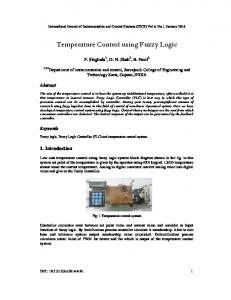
developed temperature control system using fuzzy logic. Control ... command
through serial port via microcontroller. Now, microcontroller generate PWM (
Pulse.
The aim of the temperature control is to heat the system up todelimitated
temperature, afterwardhold it ... developed temperature control system using
fuzzy logic.
developed temperature control system using fuzzy logic. Control ... calculates
actual value of PWM for heater and fan which is output of the temperature control
..... [4] The 8051 microcontroller and embedded systems using assembly and C
by ...
International Journal of Automotive Technology, Vol. 12, No. .... As LED technology continues to evolve, .... does not have a single value as membership degree.
smells and code quality. Model supporting the experimental evaluation of the fuzzy based code evaluation is implemented in Java. Key-Words: - Fuzzy Logic, ...
9. nn05_narnet - Prediction of chaotic time series with NAR neural network. 10.
nn06_rbfn_func .... For example, classify an input vector of [0.7; 1.2] p = [0.7; 1.2].
“People also do not require precise numerical input”. • These slides are based on
“Fuzzy Logic Tutorial” by. Encoder Newsletter of the Seattle Robotics Society.
Keywordsâ Fuzzy logic controller, genetic algorithm, entropy of fuzzy rules, machine learning. I. INTRODUCTION. The aim of control theory is to define a ...
of a very simple but efficient fuzzy logic based algorithm to detect the edges of an
.... example is shown when P1, P2, P3, are white and P4 is Black then output is ...
Department of Electrical and Electronic Engineering, Faculty of Engineering, Uttara. University ... solar-wind-. Diesel hybrid power system with proficient energy.
Practice "Neuro-Fuzzy Logic Systems" are based on Heikki Koivo "Neuro ...
Backpropagation and radial basis function networks are reviewed with details.
...... The following code creates a training set of inputs p and targets t for this
example.
Fuzzy Logic Examples using Matlab. Consider a very simple example: We need
to control the speed of a motor by changing the input voltage. When a set point.
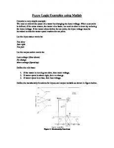
Fuzzy Logic Examples using Matlab Consider a very simple example: We need to control the speed of a motor by changing the input voltage. When a set point is defined, if for some reason, the motor runs faster, we need to slow it down by reducing the input voltage. If the motor slows below the set point, the input voltage must be increased so that the motor speed reaches the set point. Let the input status words be: Too slow Just right Too fast Let the output action words be: Less voltage (Slow down) No change More voltage (Speed up) Define the rule-base: 1. If the motor is running too slow, then more voltage. 2. If motor speed is about right, then no change. 3. If motor speed is to fast, then less voltage. Define the membership functions for inputs and output variable as shown in figure below.
Figure 1. Membership Functions
Suppose, the speed increases from the set point of 2420 to 2437.4 rpm. This is depicted on the membership function as shown below.
0.4 0.3
Figure 2. Speed above set point
The intersection points would be 0.4 and 0.3. From figure 1, we see that this speed would only intersect the rectangles consisting of rules 2 and 3. We now change the height of the triangles for input voltage.
Figure 3. Motor voltage
Now, area of “Not much change” triangle is 0.008 and area of “Slow down” triangle is 0.012. The output, as seen in Figure 3 (above), is determined by calculating the point at which a fulcrum would balance the two triangles. Thus, 0.008 X D1 = 0.012 X D2 D1 + D2 = 0.04 Solving (1) and (2) simultaneously we get, D1=0.024 D2=0.016 Thus the voltage required would be 2.40-0.024=2.376 V
(1) (2)
Let’s solve this using Matlab. Type “fuzzy” in the Matlab command prompt. Draw the appropriate membership functions as shown below:
Figure 4. Input Membership Function
Figure 5. Output Membership Function
Now set the rules 1-3 as defined earlier.
Figure 6. Rule Base
Save the file as “one.fis”. Now type in the following to get the result for the same example: fis = readfis('one'); out=evalfis(2437.4,fis) >>out = 2.376 (Same as above) Consider the next example with two inputs and one output.
Figure 7. Inverted Pendulum
Let the inputs be angle and angular velocity and the controller output be the force on the mass.
Now, define the rule base as:
Consider a scenario:
Figure 8. Memberships for angle and velocity
Let the measured angle and velocity be as shown in the figure above. We see that this will fire 4 rules: 1. If angle is zero and velocity is zero then force is zero 2. If angle is zero and velocity is NL then force is NL 3. If angle is PL and velocity is zero then force is PL 4. If angle is PL anfd velocity is NL then force is zero Now, as explained in the previous class notes,
= -0.35 N We will solve this using Matlab. Define the inputs and output similar to example 1.
Figure 9. Inputs and one output
Figure 10. Rule base
Using the same command lines as in example 1: fis = readfis('two'); out=evalfis([65 -0.1],fis) >>out = 0.3570 (same as above) We can actually visualize the output surface of the fuzzy system using the command “surfview(fis)”