Fuzzy p-values in latent variable problems by ELIZABETH A. THOMPSON Department of Statistics, University of Washington, Box 354322, Seattle, Washington 98195-4322, U. S. A.
[email protected]
and CHARLES J. GEYER School of Statistics, University of Minnesota, 313 Ford Hall, 224 Church Street S.E., Minneapolis, Minnesota, 55455, U. S. A.
[email protected]
Technical Report No. 481 Department of Statistics, University of Washington, April, 2005.
1
Summary We consider the problem of testing a statistical hypothesis where the scientifically meaningful test statistic is a function of latent variables. In particular, we consider detection of genetic linkage, where the latent variables are patterns of inheritance at specific genome locations. Fuzzy p-values, introduced by Geyer & Meeden (2005) are random variables (described by their probability distributions) that are interpreted as p-values. For latent variable problems, we introduce the notion of a fuzzy p-value as the conditional distribution of the latent p-value given the observed data, where the latent pvalue is the random variable that would be the p-value if the latent variables were observed. The fuzzy p-value provides an exact test using two sets of simulations of the latent variables under the null hypothesis, one unconditional and the other conditional on the observed data. It provides not only an expression of the strength of the evidence against the null hypothesis but also an expression of the uncertainty in that expression due to lack of knowledge of the latent variables. We illustrate these features with an example of simulated data mimicking a real example of the detection of genetic linkage. Some key words: Allele sharing; Genetic linkage; Genetic mapping; Identity by descent; Markov chain Monte Carlo; Randomised test.
2
1.
Introduction
Consider a probability model with observable variables Y and latent variables X (also called ‘missing data’ or ‘random effects’). Our interest in such models comes from the analysis of genetic data on pedigrees (Thompson, 2000) where Y is observable data on individuals and X is unobservable latent variables such as patterns of inheritance at specific genome locations. Suppose we want to do a test of significance for which a scientifically meaningful test statistic is a function t(X) of latent variables. We call this the latent test statistic. Since it cannot be observed, we cannot perform the latent test that uses it, but we can conceptualise the latent p-value of this test s(x) = pr{t(X) ≥ t(x)} (1) where the probability is calculated under the null hypothesis. For simplicity we assume in (1) that t(X) is continuous. Theory for the discrete case, which is needed for our example, is provided in Section 3. The measure of significance we propose here is the conditional distribution of s(X) given Y, which in the terminology of Geyer & Meeden (2005) is a fuzzy p-value for observed data Y. Linkage detection involves a test of whether the DNA at some location λ on a chromosome affects the trait of interest. The null hypothesis H0 is that there is no such location on the chromosome. The latent variables Xλ are patterns of inheritance at some set of locations Λ on the chromosome, and X is the vector having components Xλ . For a specific location λ the latent test statistic is t(Xλ ). We will use X0 and Y0 to denote random variables having the distributions under H0 of latent inheritance patterns and observable data, respectively. Methods for linkage detection that are robust to trait model assumptions use trait information on individuals only to specify the function t(·). The data Y consist of genetic marker data available for some members of the pedigree for some set of DNA markers at known locations on the chromosome. The standard form of the test statistics developed by Whittemore & Halpern (1994) and by Kruglyak et al. (1996) is wλ (Y) = E{t(Xλ )|Y}. The statistics wλ (Y) are typically computed at many locations λ, including the locations of the genetic markers. All available genetic marker data Y are used jointly to compute each wλ (Y). McPeek (1999) has considered alternative forms for the functions t(·) that can be used to test for genetic linkage. 3
Typically, Xλ are random given Y, even when λ is a marker location, because there are individuals for whom genetic marker data are unavailable. Also, even when marker data are complete and assumed observed without error, there may be alternative patterns of inheritance that can underlie these data. The effect of uncertainty in X on the distribution of test statistics wλ (Y) has been considered by Kruglyak et al. (1996), using measures of the expected entropy of the conditional distributions of t(Xλ ) given Y. More recently Nicolae & Kong (2004) have considered several measures of the information in Y relative to what would be available if X were observed. Although these measures can guide the collection of additional data, they do not assess directly the impact of uncertainty in X on the evidence for linkage. Even when uncertainty in X is correctly taken into account in computing the distribution under H0 of statistics wλ (Y0 ), the evidence that Y provides about X is confounded with the evidence that X provides to test the null hypothesis. Thompson & Basu (2003) first addressed this issue, introducing ‘pseudo-p-values’ based on the observed data Y and on values of Y0 simulated under H0 and having the same structure and missing-data pattern as Y. The distribution of the pseudo-p-value at location λ for the observed Y and over simulated realisations Y0 showed both the evidence for linkage and the uncertainty in t(Xλ ) given the observed Y. However, these pseudo-pvalues are not true p-values. Under H0 , the (unconditional) distribution of the pseudo-p-value is not uniformly distributed on the interval (0, 1). In this paper, we show how the latent-variable version of a fuzzy p-value defined by equation (1) expresses both the evidence in Y for testing H0 and the uncertainty about X given Y. It has several advantages over previous approaches, being both a true p-value and being conditional on Y rather than based on the distribution of Y under H0 . Although the genetic marker model enters into computation of the distribution of s(X) given Y, no simulation or consideration of Y0 is required. Additionally, the approach addresses the issue of testing over multiple chromosomal locations λ. Given the observed Y, a single conditional probability distribution both assesses the evidence concerning H0 and guides future genetic marker data collection that might clarify the truth or falsity of H0 . We illustrate our new approach using the an example of data on a single extended pedigree. This same example was previously considered by Thompson & Basu (2003).
4
2.
Testing for Genetic Linkage
Suppose we have genetic marker data Y on some individuals of a pedigree, or set of pedigrees, at a set of DNA marker loci at known locations λ ∈ ΛM . on a chromosome. We wish to test for the presence of DNA variants affecting a trait of interest: the null hypothesis (‘no linkage’) is that there are no such variants on the chromosome. In a pedigree, homologous DNA segments in different individuals are said to be identical by descent (ibd ) if they are inherited from the same DNA segment in some founder member of the pedigree. At any specific genome location λ, the pattern of ibd among pedigree members is a function of the inheritance pattern Xλ at that location. Methods for the detection of linkage between a complex disease trait and a set of genetic markers on a chromosome are based on imputed ibd among individuals who are affected for the trait. These methods exploit the fact that individuals who share the trait have increased probability of ibd at genome locations where the DNA affects trait susceptibility and hence also at linked marker loci. A test of H0 is provided by comparison of imputed ibd among affected individuals, given genetic marker data Y, with that expected given only the pedigree relationships among individuals. Specifically, ibd at location λ is measured by some function which we shall denote t(Xλ ). The latent variable considered in testing for genetic linkage is X = { Xλ : λ ∈ Λ }. Realisations of X0 , from the unconditional distribution of X under H0 , are easily simulated by ordinary i.i.d. Monte Carlo (so-called ‘gene drop’). To realise from the conditional distribution X given Y, it is best to first realise { Xλ : λ ∈ ΛM }. On small pedigrees, this can be achieved using a Baum-Welch algorithm, which is i.i.d. Monte Carlo. More generally, these realisations can be simulated by Markov chain Monte Carlo (MCMC), using methods described by Thompson (2000). If Λ is larger than ΛM , the remaining components of X may again be realised by a Baum-Welch algorithm, conditional on { Xλ : λ ∈ ΛM }. The pedigree for a small illustrative example is shown in Figure 1. The data for the example are simulated, but the form of the pedigree and data availability pattern derive from a real study (Levy-Lahad et al., 1995). There are 17 individuals affected by a disease trait (denoted ‘A’). Genetic marker data are at 10 linked marker loci spaced over a ∼ 108 bp stretch of chromosome 1. Some data are missing, as indicated in the figure legend. At location λ, Xλ specifies the inheritance of DNA from the founders of 5
Figure 1: The pedigree used in the example. ‘A’ denotes an affected individual. Dark shading indicates that the individual is typed for at least 8 of the 10 DNA marker loci. No marker data are available for the unshaded individuals, apart from two who are typed at 2 markers each.
6
the pedigree to their descendants, and hence specifies the pedigree members that share genome ibd at this location (Thompson, 2000). If Xλ were observable, a test for linkage could be based on any statistic t(Xλ ) that summarises sharing of genes ibd at location λ among affected individuals and that is expected to be larger in the presence of linkage than under H0 . In the context of robust methods for linkage detection, several such measures of latent ibd have been considered (Whittemore & Halpern, 1994; Kruglyak et al., 1996; McPeek, 1999). In our illustrative example here we consider only the simple measure used by Thompson & Basu (2003): t(Xλ ) is the size of the largest subset of affected individuals who are ibd at location λ. In the approach to this problem by earlier investigators, test statistics wλ (Y) = E{t(Xλ )|Y} are formed (Whittemore & Halpern, 1994). Alternatively, a model for the impact of linkage on t(Xλ ) (Kong & Cox, 1997) or directly on Xλ (Basu, PhD Thesis, University of Washington, 2005) may be assumed, and a likelihood-ratio-based latent test statistic formed. These statistics are typically computed at marker locations λ ∈ ΛM . On extended pedigrees, with data at multiple linked markers and marker data missing for many pedigree members, conditional expectations of ibd or likelihood-ratio based statistics can seldom be computed exactly, but a wide variety of MCMC methods have been developed (Thompson, 2000; Sobel & Lange, 1996) to realise X conditional on Y. These MCMC realisations provide Monte Carlo estimates of the desired conditional expectations { wλ (Y) : λ ∈ Λ }. An issue much discussed but seldom resolved is multiple testing. Typically the significance of wλ (Y) is assessed separately for each location λ ∈ Λ. These p-values should be corrected for multiple testing, but correction is difficult because for locations close together on a chromosome these test statistics are highly dependent. The simplest solution is to form a single statistic and use it for a single omnibus test. The natural choice in this context is the maximum over chromosomal positions: maxλ∈Λ wλ (Y). The analogous choice for the latent test statistic is t(X) = maxλ∈Λ t(Xλ ). Any computation that can be performed for the location-specific t(Xλ ) can be analogously performed for t(X). Classical parametric lod score analysis (Ott, 1999) also falls within this framework. In this case, a model for the trait data Z is assumed. The hypothesis that the DNA affecting the trait is at some location θ is tested against the alternative of independent segregation of trait and marker DNA (H0 ). These hypothesized trait locations θ may include but are distinct from locations λ at which there are marker data (ΛM ) or at which ibd is imputed 7
(Λ). The probability of marker data Y does not depend on the linkage hypothesis. Also, under the linkage alternative, Z and Y are conditionally independent given marker inheritance patterns X. Thus the base-10 loglikelihood-ratio or lod score becomes lod(θ; Y) = log10 Pθ (Z|Y) − log10 P (Z) (2) = log10 E{Pθ (Z|X)|Y} − log10 P (Z) where P (Z) is the unconditional probability density function (p.d.f.) of the trait data Z and Pθ (Z|Y) the conditional p.d.f.. This suggests the use of a latent test statistic that would be equivalent to the lod score were X observed: tθ (X) = log10 Pθ (Z|X) − log10 P (Z).
(3)
Often the maximum lod score over hypothesized trait locations θ if used as a test statistic. The analogous latent test statistic here would be maxθ tθ (X). In the standard approach, the significance of the value of any test statistic wλ (Y) or lod score lod(θ; Y) must then be assessed. On a set of pedigrees of varying structure, some form of simulation is necessary to estimate the p-value by Monte Carlo. It is easy to simulate multiple marker data sets Y0 (under H0 ) on the same pedigree structures and showing the same pattern of data availability as the observed data Y. Analysis of these data sets provides an empirical p-value, but there are several issues. First, the analysis of each simulated dataset may involve MCMC, so that for multiple simulated datasets the procedure is computationally intensive. Second, simulation of marker data sets requires some assumed marker model; specifically, we require marker locations and marker allele frequencies. On pedigrees where earlier generations are unobserved for marker data, results can be quite sensitive to assumed marker allele frequencies (Weeks & Lange, 1988). Third, since MCMC provides an estimate of the whole distribution of t(Xλ ) given Y, it seems wrong to reduce this to a single number such as the mean wλ (Y) of this distribution. Finally, the p-value based on wλ (Y) confounds uncertainty in the information which Y provides about Xλ with the evidence that Xλ provides about H0 . We see below that use of a fuzzy p-value resolves all of these issues.
3.
The Theory of Fuzzy P-values
Conventional p-values associated with test statistics are functions of data of the form (1), where x is the data and t(X) the test statistic. Equivalently, 8
we may write s(X) = pr{t(X0 ) ≥ t(X)|X}
(4)
where X0 and X are independent and X0 has the distribution of X under the null hypothesis. For simplicity, we first deal with the case where X is a continuous random vector so the probability that t(X0 ) = t(X) is zero. As mentioned in the introduction, we are interested in the case where X is an unobservable latent variable, so (4), though a useful theoretical motivation, cannot be used as is. In a context quite different from the latentvariable models considered here, Geyer & Meeden (2005) have advanced a notion of ‘fuzzy’ p-values. A random variable P is an exact fuzzy p-value if it is (unconditionally) Uniform(0, 1) distributed under the null hypothesis. Then P is less than α with probability α. Hence the randomised test based on P , which rejects the null hypothesis at level α when P ≤ α, does indeed achieve its nominal significance level. Most conventional p-values are deterministic functions of observed data, but p-values associated with classical randomised tests must be random variables (Geyer & Meeden, 2005). Here we apply the same general idea to latent-variable models and say that the random variable s(X)|Y is an exact fuzzy p-value (when X is continuous). This random variable is described by its c.d.f., which is given by F (α) = pr{s(X) ≤ α|Y}
(5a)
when X is continuous. Under H0 , the unconditional expectation of F (α) is α. More generally, when X may be discrete, we must redefine the latent test to be a randomised test with critical function of the form 0, t(x) < c ψ(x, α) = γ, t(x) = c 1, t(x) > c where c and γ are functions of x and α chosen so that Eψ(X0 , α) = α,
0 ≤ α ≤ 1.
Clearly, c is any 1 − α quantile of the distribution of t(X0 ) and γ is γ=
α − pr{t(X0 ) > c} pr{t(X0 ) = c} 9
if the denominator is nonzero (and is arbitrary otherwise). Finally, we replace (5a) by F (α) = E{ψ(X, α)|Y} (5b) in the general case (allowing for discrete X). How does one interpret a fuzzy p-value? There are two interpretations. • For a test with significance level α, F (α) given by (5a) or (5b) is the probability that the (randomised) test rejects the null hypothesis. • Alternatively, F is the c.d.f. of a continuous random variable P , which is the fuzzy p-value and summarises the strength of evidence against the null hypothesis. Just as with conventional p-values, low values are evidence against the null hypothesis, the lower the p-value, the stronger the evidence. The only difference is that now what is low or high is a distribution of values described by F . Even conventional p-values have ambiguous interpretation unless they are extreme. There is no sharp dividing line where they become ‘statistically significant.’ There is no scientifically meaningful difference between P = 0.049 and P = 0.051. The fuzziness of fuzzy p-values makes the interpretative problem no more difficult. The extremes are still easy to interpret. If the whole distribution of the fuzzy p-value is concentrated above 0.2, then there is essentially no evidence against the null hypothesis. If the whole distribution of the fuzzy p-value is concentrated below 0.01, then this is very strong evidence against the null hypothesis. The closer the distribution is to these extremes, the easier the interpretative problem. The closer the distribution is to middle values, for example, a fuzzy p-value rather uniformly distributed over the interval 0.025 < P < 0.10, the more ambiguous or equivocal the evidence about the null hypothesis.
4.
Monte Carlo Approximation
In this section we show how to calculate a fuzzy p-value by simulation, first when t(X) is continuous so no ties are possible, and then in general. If our simulations are i.i.d. then our Monte Carlo fuzzy p-values are exact. Monte Carlo evaluation of s(X) of equation (4) requires realisations of X 0 , the inheritance patterns in a pedigree, but not of marker data Y0 . These realisations may be accomplished by simulating independent realisations of the 10
multilocus meiosis process. We also require realisations from the conditional distribution of X given Y under H0 . On extended pedigrees, with extensive missing marker data, only dependent MCMC-based realisations are possible. Then our estimate of the fuzzy p-values is approximate, only converging to exact as the length of the MCMC run increases to infinity. (h) Suppose we have realisations X0 , h = 1, . . . , m, from the marginal distribution of the latent variables under the null hypothesis and realisations X(i) , i = 1, . . . , n, from the conditional distribution under the null hypothesis of the latent variables X given the observed data Y. Since X0 is independent of X and Y, s(X) of equation (4) may be rewritten as s(X) = pr{t(X0 ) ≥ t(X)|X, Y}.
(6)
Hence we can estimate this conditional probability by m
sˆ(X(i) ) =
1 X (h) I{t(X0 ) ≥ t(X(i) )} m h=1
(7)
where I{ · } is one if the term in the brackets is true and zero otherwise. Equation (7) defines n values (for i = 1, . . ., n) from the distribution of the fuzzy p-value. The empirical c.d.f. of these realisations thus provides a Monte Carlo estimate of the c.d.f. which is the fuzzy p-value. We next consider correction for continuity. Even when t(X) is a continuous random variable, this simple Monte Carlo approximation to the fuzzy p-value is not exact because of discreteness of the Monte Carlo, but a simple ‘correction for continuity’ automatically corrects for small m or n. The histogram of the sˆ(X(i) ) defined by (7) is defined to have bin boundaries k/(m + 1), k = 0, . . . , m + 1 and bin area for the k-th of these bins the (h) fraction of the X(i) such that exactly k of the t(X0 ) exceed t(X(i) ). We then consider this histogram to be the probability density function (p.d.f.) of a continuous random variable: the fuzzy p-value. To see this recipe works in general, note that under the null hypothesis, for (h) a fixed i, the t(X0 ), h = 1, . . ., m and t(X(i) ) together are an independent and identically distributed collection of continuous random variables. Hence (h) the number of t(X0 ) that exceed a particular t(X(i) ) is uniformly distributed on {0, 1, . . . , m}. Then the contribution of t(X(i) ) to the histogram is uniform over each of the bins of the histogram, hence its contribution to the histogram is Uniform(0, 1). Adding up the contributions of all the t(X(i) ) we see the fuzzy p-value is (unconditionally) Uniform(0, 1). 11
Almost the same argument holds if t(X) is discrete, and ties are broken by ‘infinitesimal jittering.’ If a particular t(X(i) ) is exceeded by exactly k (h) (h) of the t(X0 ) and tied with exactly w of the t(X0 ), then its contribution to the histogram is a rectangle having area 1/n and base with endpoints k/(m + 1) and (k + w + 1)/(m + 1). Again the contribution of each t(X(i) ) to the histogram is Uniform(0, 1) and hence so is the fuzzy p-value. Finally, we turn the histogram, a piecewise constant p.d.f., into a piecewise linear c.d.f. by integration.
5.
Application to the Linkage Example
The method of the previous section was applied to the linkage detection example of Section 2. We simulated realisations of inheritance Xλ at marker loci only, so here we have Λ = ΛM = {λ1 , . . . , λ10 }. At each marker locus, the latent test statistic t(Xλ ) used is the maximum number of affected individuals sharing genome ibd at the location of that marker. Additionally, to correct for multiple testing, we used the combined latent test statistic t(X) = maxλ∈Λ t(Xλ ). We used m = 3, 000 i.i.d. realisations of X0 and n = 30, 000 MCMC scans for the realisations of X given Y. The starting configuration for MCMC was the optimum of 3,000 sequential imputation realisations (George & Thompson, 2003). Each complete run took about 3 minutes on a 3.0 GHz Pentium PC. Clearly much longer runs are possible, as would be necessary for a larger data set consisting of multiple pedigrees. The results are shown in Figure 2. Figure 2A shows, using the full data set, the fuzzy p-value c.d.f.’s for each locus as dashed lines, and the c.d.f. for the omnibus test based on t(X) as a solid line. We see that at markers 4, 5 and 6 there is strong evidence for linkage: at marker 6, the probability the fuzzy p-value is less than 0.05 is 0.978 (not corrected for multiple testing). Although the support of the fuzzy p-value that does correct for multiple testing extends up to 0.27, the probability the fuzzy p-value is less than 0.05 is still 0.832. An interesting question in this example (and analogously much more generally) is how much of the signal derives from marker 6, which is very close to the true trait locus position in this simulated dataset. In this dataset, markers 2, 4, and 7 are the most informative (Thompson & Basu, 2003). Markers 4 and 7 are each about 1.5 × 10⁷ bp distant from marker 6, while the much less informative marker 5 is about midway between markers 4 and 12
4
1.0 7
5 6
0.6
0.6
4
B
0.8
5
0.8
1.0
A 6
0.4 0.2 0.0
0.0
0.2
0.4
7
0.00
0.10
0.20
0.00
0.10
0.20
Figure 2: Cumulative distribution functions of the fuzzy p-values for the example of Section 5 having the pedigree of Figure 1. Dashed lines are c.d.f. based on the imputed ibd at one marker locus, and solid lines are c.d.f. based on all marker loci corrected for multiple testing. A: c.d.f. using all marker data. B: c.d.f. when marker 6 data are ignored.
13
6. Figure 2B shows the same fuzzy-p-value c.d.f.’s, for the same ten marker locations, but with the data at marker 6 deleted. The signal at marker 5 drops substantially, and (as would be expected) the c.d.f. at marker 6 lies midway between those for markers 5 and 7. The signal at marker 4 drops, showing that it too was elevated by the data at marker 6, but still does provide some evidence for linkage with a median fuzzy p-value of 0.040. A fuzzy p-value having median α means the associated randomised test rejects at level α half the time. The fuzzy p-value that accounts for multiple testing (solid curve) shows very weak evidence against H0 with probability of being less than 0.05 only 0.181 and median 0.120. The fuzzy p-value provides information on the value of additional marker data collection on the same pedigree structures. In Figure 2A, not only is there a strong signal at marker 6, but also there is little uncertainty in the value of t(Xλ ) at λ = λ6 . On the other hand, had our initial data not included marker 6, the situation in Figure 2B, there would be substantial uncertainty as to underlying ibd indicating that collection of additional data might prove valuable. Typing of additional markers is usually much less costly than ascertainment of additional pedigrees, which is often not even feasible. It is of considerable practical importance to extract the potentially available information from each pedigree.
6.
Discussion
We see from these simple examples that fuzzy p-values address the four concerns regarding the deterministic (given Y) p-values of other approaches. The method is not computationally intensive, since it requires only one set of i.i.d. realisations X0 and one MCMC run yielding realisations from the conditional distribution of X given Y. No additional realisations of Y are simulated, so there is less dependence on the model for marker data. The full estimated distribution of t(X) given Y is used, and the uncertainty in the information Y provides about t(X) is reflected in the spread of the fuzzy p-value distribution. Our fuzzy p-values have a Bayesian flavor in that we consider hypotheses concerning distribution of latent variables X (which a Bayesian would call parameters) and make inferences about them using the distribution of X given observed data Y. However, there is no connection between fuzzy p-values and Bayesian p-values (posterior predictive p-values) of Rubin (1984) and 14
Meng (1994), which, like regular frequentist p-values, involve test statistics that are functions only of the observed data Y. Although our focus is the fuzzy p-value itself, as an expression of the strength of evidence against H0 , properties of the associated test are also of interest. Since the test is conditional on the observed value of Y, its validity depends only on correct distributions for X and for X|Y under H0 , and not on the marginal distribution of Y. As always, robustness comes at the expense of power. In fact, the power of the randomised test based on the latent test statistic t(X) may be either more or less powerful than the test based on E{t(X)|Y}. Whether or not t(X) is the optimal latent test statistic, the statistic E{t(X)|Y} may or may not be close to optimal. As a test constructed conditionally on the observed value of Y, our procedures share some robustness with permutation test procedures, such as those developed in this context by Churchill & Doerge (1994). Certain permutations of the components of marker data Y against the trait data Z generate multiple realisations of Y that are exchangeable under H0 . Thus, subject to this exchangeability, the permutation test shares robustness to the marginal distribution of Y with our procedure. However, the permutation procedure simply generates a distribution under H0 for the test statistic, and hence provides a classical p-value. It does not consider the distribution of any latent test statistic t(X) given the observed data Y. The fuzzy p-value expresses both the evidence in Y for testing H0 and the uncertainty about X given Y. It is the best summary of the evidence, whenever the scientifically meaningful test statistic is a function of the latent variables X. As the conditional distribution of the latent p-value given the observed data, it can be interpreted similarly to any classical p-value. At the same time, it can guide augmentation of the data Y that might reduce uncertainty in X, and hence might clarify the truth or falsity of H0 .
Acknowledgment This research was supported in part by PHS grant GM-46255, and undertaken while Dr. C. J. Geyer was visiting University of Washington on sabbatical from University of Minnesota.
15
References Churchill, G. A. & Doerge, R. W. (1994). Empirical threshold values for quantitative trait mapping. Genetics 138, 963–971. George, A. W. & Thompson, E. A. (2003). Multipoint linkage analyses for disease mapping in extended pedigrees: A Markov chain Monte Carlo approach. Statistical Science 18, 515–531. Geyer, C. J. & Meeden, G. D. (2005). Fuzzy and randomized confidence intervals and p-values. Revised and resubmitted (twice) to Statistical Science, http://www.stat.umn.edu/geyer/fuzz. Kong, A. & Cox, N. J. (1997). Allele-sharing models: LOD scores and accurate linkage tests. Am. J. Hum. Gen. 61, 1179–1188. Kruglyak, L., Daly, M. J., Reeve-Daly, M. P. & Lander, E. S. (1996). Parametric and nonparametric linkage analysis: A unified multipoint approach. Am. J. Hum. Gen. 58, 1347–1363. Levy-Lahad, E., Wijsman, E. M., Nemens, E., Anderson, L., Goddard, K. A., Weber, J. L., Bird, T. D. & Schellenberg, G. D. (1995). Familial Alzheimer’s disease locus on Chromosome 1. Science 269, 970–973. McPeek, M. S. (1999). Optimal allele-sharing statistics for genetic mapping using affected relatives. Genet. Epidemiol. 16, 225–249. Meng, X.-L. (1994). Posterior predictive p-values. Ann. Statist. 22, 1142– 1160. Nicolae, D. L. & Kong, A. (2004). Measuring the relative information in allele-sharing linkage studies. Biometrics 60, 368–375. Ott, J. (1999). Analysis of Human Genetic Linkage, 3rd ed. Baltimore, MD: Johns Hopkins University Press. Rubin, D. B. (1984). Bayesianly justifiable and relevant frequency calculations for the applied statistician. Ann. Statist. 12, 1151–1172.
16
Sobel, E. & Lange, K. (1996). Descent graphs in pedigree analysis: Applications to haplotyping, location scores, and marker-sharing statistics. Am. J. Hum. Gen. 58, 1323–1337. Thompson, E. A. (2000). Statistical Inferences from Genetic Data on Pedigrees, vol. 6 of NSF-CBMS Regional Conference Series in Probability and Statistics. Beachwood, OH: Institute of Mathematical Statistics. Thompson, E. A. & Basu, S. (2003). Genome sharing in large pedigrees: Multiple imputation of ibd for linkage detection. Human Heredity 56, 119–125. Weeks, D. E. & Lange, K. (1988). The affected pedigree member method of linkage analysis. Am. J. Hum. Gen. 42, 315–326. Whittemore, A. & Halpern, J. (1994). A class of tests for linkage using affected pedigree members. Biometrics 50, 118–127.
17