AbstractâThrough researching the operating condition of data transmission in a BitTorrent-like P2P file sharing system, we obtain two mathematical models for ...
2012 9th International Conference on Fuzzy Systems and Knowledge Discovery (FSKD 2012)
Fuzzy relation inequalities about the data transmission mechanism in BitTorrent-like Peer-to-Peer file sharing systems ShaoJun Yang
Li Jian-Xin
Faculty of Applied Mathematics, Guangdong University of Technology, Guangzhou, China Abstract—Through researching the operating condition of data transmission in a BitTorrent-like P2P file sharing system, we obtain two mathematical models for the BitTorrent-like P2P file sharing system, one ( call it (a)) relates to the system’s data transmission mechanism and the other ( call it (b)) involves the system’s optimal management. Then we study the solutions of (I), the general form of (a). Our study results show that the solutions of (a) and (b) depend on all minimal solutions of (I). Finally, by simplifying (I), we present an algorithm to search for minimal solutions of (I). Keywords P2P network; BitTorrent protocol, Mathematical model, Optimal management; Algorithm
Faculty of Applied Mathematics, Guangdong University of Technology, Guangzhou, China Suppose that the jth user A j sends the file data with quality level x j to A j , and the bandwidth between Ai and A j is aij . Because of the bandwidth limitation, the network traffic that Ai receives from A j is actually aij ∧ x j . Where, i ≠ j ,
i , j = 1, 2,..., n ; and a ij ∧ x j = min{a ij , x j } . So, the network traffic that Ai receives from the other n-1 users ( A1 , A2 ,..., Ai −1 , Ai +1 ,..., An ) is actually (see Fig.1) ai1 ∧ x1 + ai 2 ∧ x2 + … + ai ,i −1 ∧ xi −1 + ai ,i +1 ∧ xi +1 + … + ain ∧ xn
Ⅰ.INTRODUCTION Setting up the mathematic models of network communication mechanism and questing the optimal management of network communication are two important topics for network researchers. Some results have been made [1,2,3,4,5,6,7,8,9 ]. For example, two optimal mathematic models have been employed for the streaming media provider seeking a minimum cost while fulfilled the requirements assumed by a three-tier framework network using HTTP protocol. For detailed description, we refer to [1, 7]. In current time, Peer-to-Peer (P2P) networks are the mainstream for the network users in sharing information. BitTorrent (BT) protocol is one of the most widely applied P2P file transfer protocols. In a BitTorrent-like P2P file sharing system, we can utilize the computer capabilities of all the participants to share information. Each computer in the network plays two roles of both client and server, that means, each computer in the network downloads files from the other computers while simultaneously uploads files for them. In this paper, we discuss the data transmission mechanism and optimal management in BitTorrent-like P2P file sharing systems. Ⅱ.THE OPERATING CONDITION OF THE DATA TRANSMISSION IN A BITTORRENT-LIKE P2P FILE SHARING SYSTEM There are n users who are downloading some file data simultaneously, in a BitTorrent-like P2P file sharing system. Each user is guaranteed to receive the file data from the other n-1 users. Let the n users be A1 , A2 ,..., An . Now, we investigate the conditions of the ith user Ai receiving the file data from the other n-1 users.
Suppose that the quality requirement of download traffic of Ai is at least bi (bi > 0) , and then we get the conditions of the ith user Ai receiving the file data from the other n-1 users as follows, ai1 ∧ x1 + ai 2 ∧ x2 + … + ai ,i −1 ∧ xi −1 + ai ,i +1 ∧ xi +1 + … + ain ∧ xn ≥ bi i.e.
ai1 ∧ x1 + ai2 ∧ x2 +…+ ai,i−1 ∧ xi−1 + 0∧ xi + ai,i+1 ∧ xi+1 +…+ ain ∧ xn ≥ bi Hence, the n users, through a BitTorrent-like P2P file sharing system, can successfully download the file data if and only if the following inequalities hold. ⎧ 0 ∧ x1 + a12 ∧ x2 + ... + a1,i−1 ∧ xi−1 + a1,i ∧ xi + a1,i+1 ∧ xi+1 + ... + a1n ∧ xn ≥ b1 ⎪ a ∧ x + 0 ∧ x + ...a ∧ x + a ∧ x + a ∧ x + ... + a ∧ x ≥ b 2 2,i −1 i −1 2,i i +1 2,i +1 i +1 2n n 2 ⎪ 21 1 ⎪ ⎪ (a) ⎨ ⎪ ai1 ∧ x1 + ai 2 ∧ x2 + ... + ai,i−1 ∧ xi−1 + 0 ∧ xi + ai,i+1 ∧ xi+1 + ... + ain ∧ xn ≥ bi ⎪ ⎪ ⎪ ⎩an1 ∧ x1 + an2 ∧ x2 + ... + an,i−1 ∧ xi−1 + an,i ∧ xi + an,i+1 ∧ xi+1 + ... + 0 ∧ xn ≥ bn
In this application, all the quality levels x j and bandwidth
This research was supported by National Science Found of China (60974143).
978-1-4673-0024-7/10/$26.00 ©2012 IEEE
452
(2) For any j ∈ J , x ≥ b − j i
aij are normally confined to the interval [0, h], here, h is a positive number. Let I = {1, 2,..., n} and J = {1, 2,… , n} be row index set and column index set of (a) respectively, then (a) can be tersely described as follows ∑ aij ∧ x j ≥ bi , ∀i ∈ I (a) j∈J −{i}
j∈J
Where, I = {1, 2,… , m} and J = {1, 2,… , n} . Of course, (I) can be described by matrix notation, (I) A x T ≥ bT Where A = (aij ) m×n , x = ( x1 , x2 ,…, xn ) , b = (b1 , b2 ,… , bm ) , bi > 0, aij , x j ∈ [0, h] and ( ai1 , ai 2 ,..., ain ) ( x1 , x2 ,..., xn )T = ai1 ∧ x1 + ai 2 ∧ x2 + … + ain ∧ xn . 1
2
Denote X = [0, h] . For x , x ∈ X , we say x ≤ x if and only if x1j ≤ x 2j , ∀j ∈ J . In this way, the operator “ ≤ ” forms a 2
partial order relation on X and ( X , ≤) becomes a lattice. For x1 , x 2 ∈ X , we say x1 < x 2 if and only if x1 ≤ x 2 and there is some j ∈ J such that x1j < x 2j . If (I) is solvable, we denote the solution set of (I) by T X ( A, b ) = ( x1 , … , xn ) x j ∈ [ 0, h ] , j ∈ J and A xT ≥ bT .
}
Definition 1. xˆ ∈ X ( A, b) is called the greatest solution if x ≤ xˆ for all x ∈ X ( A, b) . x ∈ X ( A, b) is called a minimal solution if x ≤ x , for any x ∈ X ( A, b ) , implies x = x . Denote the set of all minimal solutions of (I) by X ( A, b) . Then it is clear that. X ( A, b) = ∪ { x ∈ X x ≤ x ≤ xˆ} . (see Lemma 2) x∈ X ( A ,b )
(I) is the general form of (a), hence, clearly, the solutions of (a) and (b) depend on all minimal solutions of (I). Theorem 1. (I) is solvable if and only if ∑aij ≥ bi , ∀i ∈ I . j∈J
∑ a ,∀i ∈I . ik
k∈J −{ j}
∑
aik ∧ xk , ∀i ∈ I .
k ∈J −{ j }
Theorem 2. Let x = ( x1 , x2 ,… , xn ) be a solution of (I). If
∑a
= bi holds for some i ∈ I , then (ai1 , ai 2 ,…, ain ) ≤ x . ∗
In the part, in order to discuss the solutions of the inequalities (a), we firstly discuss (a)’s general form, the following inequalities (I), ⎧ a11 ∧ x1 + a12 ∧ x2 + … + a1n ∧ xn ≥ b1 ⎪a ∧ x + a ∧ x + … + a ∧ x ≥ b ⎪ 21 1 22 2 2n n 2 (Ι ) ⎨ ⎪ ⎪ ⎩ am1 ∧ x1 + am 2 ∧ x2 + … + amn ∧ xn ≥ bm Where, aij , x j ∈ [0, h ], bi ∈ (0, +∞ ), i = 1, 2, … , m, j = 1, 2, … , n .The operation “+” represents the ordinary addition and a ∧ b = min{a, b} . Obviously, if a ii = 0, m = n , then the system(I) and the system (a) are equivalent. (I) can be tersely described as follows (I) ∑ aij ∧ x j ≥ bi , ∀i ∈ I .
{
(3) For any j ∈ J , a ≥ b − ij i
ij
1
∧ xk ≥ bi −
ik
j∈J
Ⅲ.THE SOLUTIONS OF (A)’S GENERAL FORM
n
∑a
k∈J −{ j}
From Theorem 1, we have Corollary 1. If (I) is solvable, then xˆ = (h, h,…, h) is the greatest solution of (I). Hereinafter, we always assume that (I) is solvable. Lemma 1. Let x = ( x1 , x2 ,…, xn ) be a solution of (I), then we have (1) x ≠ 0 .
Lemma 2. (1) Let x be a solution of (I). If x∗ ≤ x ≤ xˆ , then x is a solution of (I). (2) Let x′ be not a solution of (I). If x ≤ x′ , then x is not a solution of (I). Ⅳ.THE MINIMAL SOLUTIONS OF (I)
In this part, we discuss the minimal solutions of (I). For any j ∈ J , denote aˆ j = max{aij | i ∈ I } , and
α = (aˆ1 , aˆ2 …, aˆn ) .
Lemma 3. (1) (I) is solvable if and only if α is a solution of (I). (2) If x = ( x1 , x2 ,… , xn ) is a minimal solution of (I), then x ≤ α . Proof. (1) If (I) is solvable, then by Theorem 1, for ∀i ∈ I , a ∧ aˆ = a ≥ b , ∀i ∈ I , so, α is a a ≥ b .Then
∑
ij
∑
i
ij
∑
j
j∈J
j∈J
ij
i
j∈J
solution of (I). If α is a solution of (I), then
∑a = ∑a ij
ij
j∈J
∧ aˆ j ≥ bi , ∀i ∈ I , and
j∈J
by Theorem 1, (I) is solvable. (2)If ∃j0 ∈ J such that x j > aˆ j , then let 0
0
x′ = ( x1, x2 ,...x j −1, aˆ j , x j +1,..., xn ) and then we get x > x ' . Because x j > aˆ j ≥ aij , when x′ is substituted into(I), for ∀i ∈ I , we get 0
aij0 ∧ aˆ j0 +
∑
j∈J −{ j0 }
aij ∧ x j = aij0 ∧ x j0 +
∑
j∈J −{ j0 }
0
0
aij ∧ x j = ∑ aij ∧ x j ≥ bi . j∈J
That is to say, x′ is a solution of (I), a contradiction to that x is a minimal solution of (I).■ Theorem 3. Let x = ( x1 , x2 ,… , xn ) be a minimal solution of (I), then there is some i ∈ I such that ∑a ∧ x = b . ij j i j∈J
Proof. Denying the thesis, let us assume that for ∀i ∈ I , a ∧ x > b . By Lemma 1, x ≠ 0 , hence, ∃j0 ∈ J such that
∑
ij
j
i
j∈J
x j0 > 0 . Due to Lemma 1(2),(3) and the above assumption, we get the following a) and b) , a) a > b − ∑ aij ∧ x j , ∀i ∈ I . ij0 i j∈J −{ j0 }
b) x > b − j0 i
∑
aij ∧ x j , ∀i ∈ I .
j∈J −{ j0 }
Denote x′ = max{0, b − j0 i
∑
aik ∧ xk | i ∈ I} . From b) , we
k∈J −{ j0 }
get x j > x′j . Let x ' = (x1, x2 , , x j −1, x′j , x j +1,..., xn ) , then 0 0 0 0 0 x > x′ . When x′ is substituted into (I), with the definition of and a), we get ′ x j0 aij0 ∧ x ′j0 + = bi −
∑
∑
j ∈ J −{ j 0 }
j ∈ J −{ j 0 }
aij ∧ x j ≥ aij0 ∧ (bi −
aij ∧ x j +
∑
j∈ J −{ j0 }
∑
aij ∧ x j ) +
j∈ J −{ j0 }
aij ∧ x j = bi ,
∑
aij ∧ x j
j ∈ J −{ j 0 }
∀i ∈ I
Hence, x ' is also a solution of (I), it is a contradiction to the
453
fact that x is a minimal solution of (I).■ Let x = ( x1 , x2 , xn ) be a solution of (I), and denote
That is to say, i ∈ I ( x) , so I ( x ) ⊆ I ( x ) . (3)If x j = max{aij | i ∈ I ( x)} , then ∃i0 ∈ I (x) ⊆ I (x) satisfying
I ( x) = {i ∈ I | ∑ aij ∧ x j = bi } , J i ( x) = { j ∈ J | aij < x j }, i ∈ I ( x) .
x j0 = ai0 j0 , then j0 ∉ J i ( x ) , and j0 ∉ ∩ Ji ( x) .
j∈J
0
0
0
If x = max{(b − j0 i
Clearly, we have I ( x) = {i ∈ I | a ∧ x > b }. ∑ ij j i j∈J
Theorem 3 can be expressed as follows. Theorem 3’. Let x = ( x1 , x2 ,… , xn ) be a minimal solution of (I), then I ( x) ≠ ∅ . Lemma 4. Suppose x = ( x1 , x2 ,… , xn ) is a solution of (I),
that x =b − j0 i0 have
∑a
i0 j
j∈J
∑a
j∈J−{ j0}
i∈I ( x )
x j0 = max{max{aij0 | i ∈ I ( x)}, max{(bi −
aij ∧ x j ) | i ∈ I ( x)}} .
∑
j∈J −{ j0 }
, x j0 , x j0 +1 ,..., xn ) < x , and x is a 0 −1
Then, (1) x = ( x1 , x2 ,..., x j solution of (I) also. (2) I ( x) ⊆ I ( x) . (3) j ∉ ∩ J ( x) . 0
ai0 j0 ≥ ai0 j0 ∧ xj0 > bi0 −
ai0 j0 ∧ x j0 + = (bi0 −
i∈I ( x )
aij ∧ xj and xj0 > bi −
x j0 > max{(bi −
aij ∧ xj , ∀i ∈ I ( x) .
∑
j∈J −{ j0 }
∑
j∈J −{ j0 }
{
aij ∧ x j ) | i ∈ I ( x)} ≥ bi −
{
∑
On the other hand, by Lemma 1, a ≥ b − ij i 0
j∈J −{ j0 }
aij ∧ x j ) +
j∈J −{ j0 }
∑
j∈J −{ j0 }
aij ∧ x j .
∑
aij ∧ x j .
∑
aij ∧ x j
j∈J −{ j0 }
j∈J −{ j0 }
{
}
aij0 ∧ x j0 = aij0 = aij0 ∧ x j0 .
Hence,
ai1 ∧ x1 + ai 2 ∧ x2 + … + ai , j0 −1 ∧ x j0 −1 + aij0 ∧ x j0 + ai , j0 +1 ∧ x j0 +1 + … + ain ∧ xn
= aij0 ∧ x j0 +
∑
j∈J −{ j0 }
aij ∧ x j = aij0 ∧ x j0 +
∑
aij ∧ x j = bi , ∀i ∈ I ( x)
j∈J −{ j0 }
Therefore, by the above 1) and 2), we have proved that x is a solution of (I). (2) For any i ∈ I ( x ) , by (1) , we have x j > x j ≥ aij , so 0 0 0 aij0 ∧ x j0 +
∑
j∈J −{ j0 }
= aij0 ∧ x j0 +
∑
aij ∧ x j = aij0 +
j∈J −{ j0 }
i∈I ( x )
i∈I ( x)
i∈I ( x )
Theorem 4. Let x = ( x1 , x2 ,… , xn ) be a solution of (I), then x is a minimal solution of (I) if and only if I ( x) ≠ ∅ and ∩ J ( x) = ∅ . i∈I ( x)
i
Proof. Suppose that x is a minimal solution of (I). Then according to Theorem 3’, we know that I ( x) ≠ ∅ . If ∩ Ji (x) ≠ ∅, i∈I ( x)
then, according to Lemma 4(1), x is not a minimal solution, and this is a contradiction to the supposition. Hence, ∩ Ji (x) =∅. i∈I ( x)
x j0 > x j0 ≥ max aij0 | i ∈ I ( x ) ≥ aij0 ,
then
i∈I ( x )
i∈I ( x )
aij ∧ x j = bi , ∀i ∈ I ( x )
2) For any i ∈ I ( x) , we have
0
i∈I ( x )
Hence, when x is substituted into the ith inequality of (I), we have
∑
0
∩ Ji ( x) ⊂ ∩ Ji ( x) .■
j∈ J −{ j0 }
aij ∧ x j ) +
}
By (1), the only difference between x and x is the j0th term: x j > x j ≥ aij . Hence, J i ( x) ⊆ J i ( x) . And then to (3), we have j ∈ ∩ J ( x) , but j ∉ ∩ J (x) , hence 0 i 0 i
j∈J −{ j0 }
∑
}
Ji (x) = j aij < xj , xj ∈{x1, x2 ,..., xj0 −1, xj0 , xj0 +1,..., xn} .
i∈I ( x )
j∈J −{ j0 }
aij ∧ x j ≥ aij0 ∧ (bi −
i∈I ( x )
∩ J i ( x) ⊆ ∩ J i ( x) ⊆ ∩ J i ( x) . On the other hand, according
Now, we prove that x is a solution of (I) also. 1) For any i ∈ I ( x) ,
= (bi −
ai0 j ∧ x j = bi0 .
i∈I ( x )
0
aij ∧ x j ) | i ∈ I ( x)} .
∑
So, x j < x j .and then we get x < x . 0 0
∑
∑
j∈J −{ j0 }
ai0 j ∧ x j
i
and
Hence
aij0 ∧ x j0 +
ai0 j ∧ x j ) +
∑
j∈J −{ j0 }
Ji (x) = j aij < xj , xj ∈{x1, x2 ,..., xj0 −1, xj0 , xj0 +1,..., xn}
∑ aij ∧ x j > bi , then
x j0 ≥ max{(bi −
∑
ai0 j ∧ x j = x j0 +
i ∈ I ( x) , let us examine
j∈J
j∈J −{ j0 }
∑
j∈J −{ j0 }
j∈J −{ j0 }
i∈I ( x )
i ∈ I ( x) , hence, x j0 > max{aij0 | i ∈ I ( x)} .
∑
ai0 j ∧ xj = xj0 .
(4) By (2), I ( x ) ⊆ I ( x ) , then ∩ J ( x) ⊆ ∩ J ( x) . For any i i
i∈I ( x )
aij0 ∧ xj0 > bi −
∑
j∈J −{ j0 }
It gives two facts: 1) ai j > x j and 2) 0 0 0
0
Proof. (1)For any j ∈ ∩ J ( x) , we have x j > aij ≥ 0 , 0 i 0 0
For any i ∈ I ( x ) ,
∧xj . With the definition of I ( x) , we
0
(4) ∩ J ( x) ⊂ ∩ J ( x) . i i i∈I ( x )
aij ∧ x j ) | i ∈ I ( x)} , then ∃i0 ∈ I ( x) such
2) and 1) mean that i0 ∈ I ( x) and j0 ∉ Ji (x) . Hence, j ∉ ∩ J ( x) .
i
i∈I ( x )
∑
j∈J −{ j0 }
∧ x j > bi0 , hence,
I ( x) ≠ ∅ and ∩ J i ( x) ≠ ∅ . For any j0 ∈ ∩ J i ( x ) , denote i∈I ( x )
i0 j
i∈I ( x)
∑
j∈J −{ j0 }
aij ∧ x j
Now, suppose that I ( x) ≠ ∅ and ∩ Ji ( x) = ∅ . We prove i∈I ( x )
that x is a minimal solution of (I). If there is a x′ = ( x1′, x2′ ,… , xn′ ) ∈ X ( A, b) such that x′ < x . It means x′j ≤ x j , ∀j ∈ J and there is some j0 ∈ J such that x′j < x j . 0 0 There is at least a i0 in I ( x) such that j0 ∉ J i ( x ) (otherwise, we have ∩ J (x) ≠ ∅ , a contradiction to the above supposition) . 0
i∈I ( x)
i
That is to say
∑a Hence, we have
ai0 j ∧ x j = bi0 .
454
k ∈J
i0 k
∧ xk = bi0 and x j0 ≤ ai0 j0 .
∑a
i0 j
j∈J
∧ x′j =ai0 j0 ∧ x′j0 +
= x′j0 +
∑
j∈J −{ j0 }
= ai0 j0 ∧ x j0 +
∑
j∈J −{ j0 }
ai0 j ∧ x j < x j0 +
∑
j∈J −{ j0 }
ai0 j ∧ x′j ≤ ai0 j0 ∧ x′j0 +
∑
j∈J −{ j0 }
∑
j∈J −{ j0 }
ai0 j ∧ x j
j∈ J ∗ − { s }
ai0 j ∧ x j = bi0
∑a
ij
si
∑a
< bi and
ij
j =1
s
i
= bi −
ij
(I*)
∧ xj ≥ bi , ∀i ∈I
We call (I*)the critical inequalities of (I). Clearly, the following Lemma holds. ∗ Lemma 5. If x = ( x1 , x2 ,… , xs ) is a minimal solution of (I*), then x = ( x1 , x2 ,…, xs ,0,0,…,0) (here, n-s zeros) is a minimal solution of (I). According to Lemma 5, once we get a minimal solution of (I*), we can get a minimal solution of (I) accordingly. Denote IS = {i ∈ I | si = s} , according to the definition of s ,
(2) Denote a′ = max{b − s i i∈I S
∑
j∈J ∗ −{s}
as follows
j∈J ∗
we get 0 < bi −
∑
aij = bi −
∗
j∈J −{ s}
∑
∑
i
j∈J ∗
ij
i
j∈J −{ s }
i∈I S
∑
j∈J ∗ −{ s }
aij } ≤ max{ais } ≤ max{ais } = aˆs . i∈I S
i∈I
So, α ′ ≤ αˆ . Now we prove α ′ is a solution of (I*). 1) For any i ∈ I S , from the above proof, we have the results: as′ ≥ bi − a is ∧ a s′ + = bi −
∑
j∈ J ∗ − { s }
∑
j∈ J ∗ −{ s }
∑
j∈J ∗ −{ s }
aij and ais ≥ bi −
a ij ∧ aˆ j ≥ a is ∧ ( bi −
a ij +
∑
j∈ J ∗ − { s }
aij ∧ aˆ j = bi .
ij
s} , then set up inequalities (I*)
∧ x j ≥ bi , i ∈ I
(I*)
∑
j∈J ∗ −{ s}
aij } .Then let
α 1 = ( a11 , a12 ,..., a1s −1 , a1s ) = (aˆ1 , aˆ2 ,..., aˆ s −1 , a1s ) . Then set up I (α 1 ) and ∩ J i (α 1 ) (according to Lemma i∈I (α 1 )
6(3), I (α 1 ) ≠ ∅ ). If
1 ∩ Ji (α1) =∅, then according to Theorem 4, α is a
minimal solution of (I*), and denote x = α 1 . Go to Process 4. If ∩ Ji (α1 ) ≠ ∅ , then go to Step 2. 1 i∈I (α )
Step 2. Because ∩ Ji (α1 ) ≠ ∅ , then let 1 i∈I (α )
j2 = max ∩ 1 Ji (α ) and compute 1
i∈I (α )
Hence, 0 < as′ = max{bi −
aij ∧ aˆ j
i∈I (α1 )
aij ∧ aˆ j ≤ ais ∧ aˆ s = ais , ∀i ∈ I S .
∗
∑
j∈J ∗ −{ s }
∑
j∈J ∗ −{ s }
Process 3. Search for minimal solutions of (I*). Step 1. Compute αˆ = (aˆ1 , aˆ2 aˆ s ) and
aij } and let
ij
∑a
i∈I S
Proof. (1) The conclusion is true by Lemma 3. (2) For any i ∈IS we have a ≥ b , then a < b and
∑
aij ∧ aˆ j +
i∈I
(ai1 , ai 2 ,..., ai ,s −1 , ais ) α ′ = bi .
j∈J ∗ −{s}
∑
j∈ J ∗ −{ s }
a ij ∧ aˆ j ≤ a is ∧ aˆ s ≤ a is .
aij ∧ aˆ j = as′ +
and s = max{si } , J * = {1, 2,
a1s = max{bi −
α ′ = ( aˆ1 , aˆ 2 ,..., aˆ s −1 , as′ ) , then α ′ ≤ αˆ and α ′ is a solution of (I*). (3)There is some i ∈ I S such that
j∈J ∗ −{ s }
∑
j∈ J ∗ − { s }
i.e., (ai1 , ai 2 ,..., ai , s −1 , ais ) α ′ = bi .■ Based on the concepts and results discussed above, we present an algorithm to search for minimal solutions of (I). Process 1. Check (I)’s feasibility. Compute α = (aˆ1 , aˆ2 aˆn ) . If α is a solution of (I), then by Lemma 2, (I) is solvable, and go to Process 2. Otherwise, stop. Process 2. Set up inequalities(I*). According to Definition 2, we compute si , i ∈ I ,
we have IS ≠ ∅.
Lemma 6. (1) αˆ = ( aˆ1 , aˆ2 ,..., aˆs ) is a solution of (I*).
a ij = bi −
∑
ais ∧ as′ +
i∈I
j∈J∗
j∈ J ∗ − { s }
Then,
≥ bi , then we call si a critical number of the
∑a
aij ∧ aˆ j ≥ bi . That is to say, α ′ satisfies the ith
∑
a s′ = bi −
ith inequality of (I). Specially, if ai1 ≥ bi , then si = 1 . Denote s = max{si } , J ∗ = {1, 2, …, s} , let us consider the
a ij ≥ bi , of course,
ij
j∈J ∗ −{s}
j =1
following system
j∈J ∗ −{ s}
j∈ J ∗ − { s }
inequality. Therefore, by 1) and 2), we deduce that α ′ is a solution of (I*). (3)According to the definition of a′s , ∃i ∈ I S such that a′ = b − ∑ a . On the other hand, with (1) we have
Ⅴ.AN ALGORITHM FOR (I)
In this part, we first simplify(I), and then present an algorithm to search for minimal solutions of (I). Definition 2. For i ∈ I , if there is a si ∈ J such that
∑
a ij ∧ aˆ j =
∑
ais ∧ as′ +
ai0 j ∧ x j
The above inequality means that x ' does not satisfy the i0th inequality of (I), a contradiction to the hypothesis x′∈ X ( A, b) .■
si −1
∑
have
a ij = bi .
So, α ′ satisfying the ith inequality. 2)For any i ∈ I − I S , we
∑
j∈J ∗ −{ s}
∑
j∈ J ∗ − { s }
aij . Hence,
a ij ) +
∑
j∈ J ∗ −{ s }
a = max{max{aij2 | i ∈ I (α1 )},max{(bi − 2 j2
aij ∧ a1j ) | i ∈ I (α1 )}} .
Denote α 2 = (a12 , a22 ,...,, as2 ) = (aˆ1, aˆ2 ,..., aˆ , a , aˆ j +1,..., aˆs−1, a1s ) . 2 According to Lemma 4, we know that: α 2 < α 1 and α 2 is a solution of (I*) also. Set up I (α 2 ) and ∩ J i (α 2 ) . i∈I (α 2 )
If a ij
∑
j∈J ∗ −{ j2 } 2 j2 −1 j2
2 ∩ Ji (α ) = ∅ , then according to Theorem 4, α is a 2
i∈I (α 2 )
minimal solution of (I*), and denote x = α 2 . Go to Process 4. If ∩ J (α2 ) ≠ ∅ , then go to Step 3. i∈I (α 2 )
i
Step 3. Because ∩ J (α 2 ) ≠ ∅ , then let j = max ∩ J (α 2 ) , i 3 i 2 i∈I (α )
and compute
455
i∈I (α 2 )
a3j3 = max{max{aij3 | i ∈ I (α 2 )}, max{(bi −
∑
j∈J ∗ −{ j3 }
aij ∧ a2j ) | i ∈ I (α 2 )}} .
Denote α 3 = (a13 , a23 ,...,, as3 ) = (aˆ1, aˆ2 ,..., aˆ j3 −1, a3j3 , aˆ j3 +1,..., aˆ j2 −1, a2j2 , aˆ j2 +1,..., aˆs−1, a1s ) According to Lemma 4, we know that: α 3 < α 2 and α3 is also a solution of (I*). Set up I (α3 ) and ∩ Ji (α 3 ) . 3 i∈I (α )
If
∩ Ji (α ) = ∅ , then according to Theorem 4, 3
i∈I (α 3 )
α is a 3
minimal solution of (I*), and denote x = α 3 . Go to Process 4. If ∩ J (α 3 ) ≠ ∅ , then go to Step 4. i
i∈I (α 3 )
…… Continue in order, according to the above-mentioned manners. Now, among aˆ1 , aˆ2 ,..., aˆs , let us consider those special members that satisfy aij < aˆ j , for some j ∈ J * , some i ∈ I . Because s is a finite number, then the number of those special members is finite (≤ s ) . On the other hand , by Lemma 4(2),(4), we know that ∅ ≠ ∩ 1 J i (α 1 ) ⊃ ∩ 2 J i (α 2 ) ⊃ ∩ 3 J i (α 3 ) ⊃ ... i∈I (α )
i∈I (α )
i∈I (α )
and
Process 2. According to Definition 2, find s1 = 3, s2 = 5, s3 = 4, s4 = 5, s5 = 5 , s = max{si | i ∈ I } = 5, J ∗ = {1, 2, 3, 4, 5} . Process 3. Step 1. I S = {i ∈ I | si = s} = {2, 4,5} , a1s = max{bi − i∈I S
∑
j∈J ∗ −{5} 1 1 4 5
aij } = max{0.6, 0.4, 0.4} = 0.6 ,
α1 = (a11, a12 , a31, a , a ) = (0.9,0.9,0.8,0.7,0.6) , I (α 1 ) = {i ∈ I | (ai1 , ai 2 , ai 3 , ai 4 , ai5 ) α 1 = bi } = {2} and J 2 (α 1 ) = { j ∈ J * | a2 j < a1j } = {1, 2, 3, 4} , then
∩ J i (α 1 ) = {1, 2, 3, 4} .
i∈I (α 1 )
Step 2. j = max ∩ J (α 1 ) = 4 , 2 i 1 i∈I (α )
2 a42 = 0.5 , α 2 = (0.9, 0.9,0.8,0.5, 0.6) , I(α ) ={2,5}, J 2 (α 2 ) = {1, 2, 3, 4} ,
J 5 (α 2 ) = {2,3} , then
∩
i∈ I (α 2 )
J i (α 2 ) = {2, 3} .
Step 3. j3 = max ∩ J i (α 2 ) = 3 , 2 i∈I (α )
3 3 a33 = 0.6 , α = (0.9,0.9,0.6,0.5,0.6) , I (α ) = {2,4,5},
J 2 (α 3 ) = {1, 2, 3, 4} , J 4 (α 3 ) = {1} and J 5 (α 3 ) = {2,3} ,
then
∩ Ji (α 3 ) = ∅ .
i∈I (α 3 )
∅ ≠ I (α 1 ) ⊆ I (α 2 ) ⊆ I (α 3 ) ⊆ ... ,
hence, certainly, there is a l in {1, 2,…, s} such that l ∩ J i (α l −1 ) ≠ ∅ and ∩ Ji (α ) = ∅ . So, we have the i∈I (α l )
i∈I (α l −1 )
following Step l. Step l. Because ∩
i∈I (α l −1 )
let j = max l
By theorem 4, x = α 3 is a minimal solution of (I*). Process 4. x = ( x, 0) = (0.9, 0.9, 0.6, 0.5, 0.6, 0) is a minimal solution of (I)■
∩
i∈I (α l −1 )
REFERENCES
J i (α l −1 ) ≠ ∅ , then
J i (α l −1 ) , and compute
aljl = max{max{aijl | i ∈ I (α l −1 )}, max{(bi −
∑
j∈J ∗ −{ jl }
[2]
aij ∧ alj−1 ) | i ∈ I (α l −1 )}}
Denote α l = (a1l , a2l ,..., , asl ) = (aˆ1 , aˆ2 ,..., aˆ jl −1 , a ljl , aˆ jl +1 ,..., aˆ jl−1 −1 ,
a ljl−−11 , aˆ jl −1 +1 ,..., aˆ j3 −1 , a 3j3 , aˆ j3 +1 ,..., aˆ j2 −1 , a 2j2 , aˆ j2 +1 ,..., aˆs −1 , a1s ) According to Lemma 4(1), we know that: α l < α l −1 and α l is also a solution of (I*). Set up I (αl ) and ∩ J (α l ) . i i∈I (α l )
Because
[1]
[3] [4]
[5]
[6]
∩ Ji (α ) = ∅ , then according to Theorem 4, l
i∈I (α l )
α is a minimal solution of (I*), and denote x = α l . Go to Process 4. Process 4. Find a minimal solution of (I). According to Lemma 5, ( x,0,0,…,0) (n-s zeros) is a l
minimal solution of (I).
[7]
[8]
[9]
Ⅵ.EXAMPLE Example 1.Consider the following problem. ⎛ x1 ⎞ ⎜ ⎟ ⎛1.5 ⎞ ⎜ x2 ⎟ ⎜ 2.0 ⎟ 0.4 ⎟ ⎜ x3 ⎟ ⎜ (Ι ) 0.7 ⎜ ⎟ ≥ ⎜1.8 ⎟ ⎜ x4 ⎟ ⎜ 2.9 ⎟ 0.5 ⎟ ⎜x ⎟ ⎜ ⎜ 5 ⎟ ⎜⎝ 2.6 ⎟⎠ 0.7 ⎜x ⎟ ⎝ 6⎠ Solution. I = {1, 2,3, 4,5}, J = {1, 2,3, 4,5, 6}, h = 3 . Process 1. α = (0.9, 0.9, 0.8, 0.7, 0.8, 0.4) . Because ⎛ 0.8 0.3 0.5 ⎜ ⎜ 0.5 0.2 0.3 ⎜ 0.3 0.6 0.2 ⎜ ⎜ 0.3 0.9 0.8 ⎜ 0.9 0.5 0.1 ⎝
0.2
0.1 0.3 ⎞ ⎟ 0.7 0.2 ⎟ 0.3 0.4 ⎟ ⎟ 0.8 0.1 ⎟ 0.8 0.2 ⎟⎠
α satisfies (I), then, by Lemma 3, (I) is solvable.
456
H.-C. Lee, S.-M. Guu, On the optimal three-tier multimedia streaming services, Fuzzy Optim. Decision Making 2 (31) (2002) 31–39. Y.-K.Wu, S.-M. Guu, Minimizing a linear function under a fuzzy max–min relational equation constraint, Fuzzy Sets and Systems 150 (2005)147–162. S.-C. Fang, G. Li, Solving fuzzy relation equations with a linear objective function, Fuzzy Sets and Systems 103 (1999) 107–113. Y.-K. Wu, S.-M. Guu, J.Y.-C. Liu, An accelerated approach for solving fuzzy relation equations with a linear objective function, IEEE Trans.Fuzzy Systems 10 (4) (2002) 552–558. J.-X. Li, A new algorithm for minimizing a linear objective function with fuzzy relation equation constraints,Fuzzy Sets and Systems (2008), doi: 10.1016/j.fss.2008.02.017. J.-X. Li, G. Hu, A New Algorithm for Minimizing a Linear Objective Function Subject to a System of Fuzzy Relation Equations with Max-product Composition,Fuzzy Inf. Eng. (2010)DOI. 1007/s 12543010-0050-9. Li J X, Hu G, An algorithm for fuzzy relation equations with max-product composition. Advances in Fuzzy Sets and Systems 4(1),(2009) 1-21. J. Loetamonphong and S.-C. Fang, Optimization of fuzzy relation equations with max-product composition, Fuzzy Sets and Systems 118(2001) 509-517. Ghodousian A, Khorram E (2006) An algorithm for optimizing the linear function with fuzzy relation equation constraints regarding max-prod composition. Applied Mathematics and Computation 178:502-509.