Fuzzy Self-Localization using Natural Features in the Four-Legged

Fuzzy Self-Localization using Natural Features in the Four-Legged League? D. Herrero-P´erez1 , H. Mart´inez-Barber´a1 , and A. Saffiotti2 1

Dept. Information and Communication Engineering, University of Murcia, 30100 Murcia, Spain [email protected] [email protected] 2 Dept. of Technology ¨ ¨ Orebro University, 70218 Orebro, Sweden [email protected]

Abstract. In the RoboCup four-legged league, robots mainly rely on artificial coloured landmarks for localisation. As it was done in other leagues, artificial landmarks will soon be removed as part of the RoboCup push toward playing in more natural environments. Unfortunately, the robots in this league have very unreliable odometry due to poor modeling of legged locomotion and to undetected collisions. This makes the use of robust sensor-based localization a necessity. We present an extension of our previous technique for fuzzy self-localization based on artificial landmarks, by including observations of features that occur naturally in the soccer field. In this paper, we focus on the use of corners between the field lines. We show experimental results obtained using these features together with the two nets. Eventually, our approach should allow us to migrate from landmarks-only to line-only localisation. Keywords: Autonomous robots, fuzzy logic, image processing, localization, state estimation.

1

Introduction

The current soccer field in the Four-Legged Robot League has a size of approximately 4, 5m · 3m, and the only allowed robot is the Sony AIBO [10]. The exteroceptive sensor of the robot is a camera, which can detect objects on the field. Objects are color coded: there are four uniquely colored beacons, two goal nets of different color, the ball is orange, and the robots wear colored uniforms. However, in a real soccer field there are not characteristic colored cues. The rules of RoboCup are gradually changed year after year in order to push progress toward the final goal. Removal of the artificial colored beacons will be the next step in this direction. Accordingly, some preliminary development has been done by some teams in this league to allow the robot to self-localize without using the artificial beacons. ?

To appear in: D. Nardi, M. Riedmiller and C. Sammut (eds) RoboCup 2004: Robot Soccer World Cup VIII. Springer-Verlag, DE, 2004.

For instance, the German Team uses a sub-sampling technique to detect pixels that belong to the field lines. These pixels are used in a Monte-Carlo localisation (MCL) schema [4]. MCL is a probabilistic method, in which the current location of the robot is modeled as the density of a set of particles. Each particle can be seen as the hypothesis of the robot being located at that position. Using only a small number of samples, it increases the stability of the localization by maintaining separate probabilities for different edge types for each sample. These probabilities are only adapted slowly. This paper describes the process of self-localization using the field lines as a source of features. In fact, what it is used are the corners produced by the intersection of the field lines, instead of the classical approach of using the line segments. Then, these corners are treated as natural landmarks in a technique based on [5], which uses fuzzy logic to account for errors and imprecision in visual recognition of landmarks and nets, and for the uncertainty in the estimate of robot’s displacement. This technique allows for large odometric errors and inaccurate observations with excellent results. However, it should be noted that the idea of corner-based localisation presented here could also be incorporated into other localisation approaches, like MCL.

2

Perception

The AIBO robots [10] use a CCD camera as the main exteroceptive sensor. The perception process is in charge of extracting convenient features of the environment from the images provided by the camera. As the robot will localize relying on the extracted features, both the amount of features detected and their quality will clearly affect the process. Currently the robots rely only on coloured landmarks for localization, and thus the perception process is based on color segmentation for detecting the different landmarks. Soon artificial landmarks will be removed, as it was done in other leagues. For this reason, our short term goal is to augment the current landmark based localization with information obtained from the field lines, and our long term goal is to rely only on the field lines for localisation. Because of the League rules all the processing must be done on board and for practical reasons it has to be performed in real time, which prevents us from using time consuming algorithms. A typical approach for detecting straight lines in digital images is the Hough Transform and its numerous variants. The various variants have been developed to try to overcome the major drawbacks of the standard method, namely, its high time complexity and large memory requirements. Common to all these methods is that either they may yield erroneous solutions or they have a high computational load. Instead of using the field lines as references for the self-localization, we decided to use the corners produced by the intersection of the field lines (which are white). The two main reasons for using corners is that they can be labeled (depending on the type of intersection) and they can be tracked more appropriately given the small field of view of the camera. In addition, detecting corners

can be more computationally efficient than detecting lines. There are several approaches, as reported in the literature, for detecting corners. They can be broadly divided into two groups: – Extracting edges and then searching for the corners. An edge extraction algorithm is pipelined with a curvature calculator. The points with maximum curvature (partial derivative over the image points) are selected as corners. – Working directly on a gray-level image. A matrix of “cornerness” of the points is computed (product of gradient magnitude and the rate of change of gradient direction), and then points with a value over a given threshold are selected as corners. We have evaluated two algorithms that work on gray-level images and detect corners depending on the brightness of the pixels, either by minimizing regions of similar brightness (SUSAN) [8] or by measuring the variance of the directions of the gradient of brightness [9]. These two methods produce corners, without taking into account the color of the regions. As we are interested in detecting field lines corners, the detected corners are filtered depending on whether they come from a white line segment or not. The gradient based method [9] is more parametric, produces more candidate points and requires similar processing capabilities than SUSAN [8], and thus it is the one that we have selected to implement corner detection in our robots. Because of the type of camera used [10], there are many problems associated to resolution and noise. The gradient based method detects false corners in straight lines due to pixelation. Also, false corners are detected over the field due to the high level of noise. These effects are shown in Fig. 1 (a). To cope with the ˙ shows noise problem, the image is filtered with a smoothing algorithm. Fig. 1(b) the reduction in noise level, and how it eliminates false detections produced by this noise (both for straight lines and the field).

(a)

(b)

Fig. 1. Brightness gradient-based detector. (a) From raw channel. (b) From smoothed channel. The detected corners are indicated by a white small square.

The detected corners are then filtered so that we keep only the relevant ones, those produced by the white lines over the field. For applying this color filter,

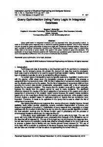
we first segment the raw image. Fig. 2 (b) shows the results obtained using a threshold technique for a sample image. We can observe that this technique is not robust enough for labeling the pixels surrounding the required features. Thus, we have integrated thresholding with a region-based method, namely the Seed Region Growing (SRG), by using the pixels classified by the a conservative thresholding as seeds from which we grow color regions. (See [11] for details.) The resulting regions for our image are shown in Fig. 2 (c). Finally, we apply a color filter for all corners obtained with the gradient-based method. We show in Fig. 2 (d) the corners obtained with the gradient-based method (white) and the corners that comply with the color conditions (black).

(a)

(b)

(c)

(d)

Fig. 2. Feature detection. (a) RGB image. (b) Segmented image by thresholding. (c) Segmented image by seeded region growing. (d) Gradient-based detected corners (white) and color-based filtered corners (black). The two detected corner-features are classified as a C and a T, respectively.

Once we have obtained the desired corner pixels, these are labeled by looking at the amount of field pixels (carpet-color) and line or band pixels (white) in a small window around the corner pixel. Corners are labeled according to the following categories. Open Corner A corner pixel surrounded by many carpet pixels, and by a number of white pixels above a threshold. Closed Corner A corner pixel surrounded by many white pixels, and by a number of carpet pixels above a threshold. Net Closed Corner A corner surrounded by many white pixels, and by a number of carpet and net (blue or yellow) pixels above a threshold. Note that in order to classify a corner pixel, we only need to explore the pixels in its neighborhood. From these labeled corners, the following features are extracted. Type C An Open corner nearby of a closed corner. This feature can be detected in the goal keeper area of field. Type T-field Two closed corner. Produced by the intersection of the walls and the inner field lines.

Type T-net A closed corner nearby of a net closed corner. Produced by the intersection of goal field lines and the net. In Fig. 2 (d), four detected corner pixels have been combined into two cornerfeatures, respectively classified as a C and a T-field. The resulting corner-features, together with the landmarks and the nets, are used for localizing a robot in the field. In the rest of this paper, we show how to represent the uncertainty associated to these features, and how to use these features in our fuzzy localization technique in order to obtain an estimate of the robot position.

3 3.1

Uncertainty Representation Fuzzy locations

Location information may be affected by different types of uncertainty, including vagueness, imprecision, ambiguity, unreliability, and random noise. An uncertainty representation formalism to represent locational information, then, should be able to represent all of these types of uncertainty and to account for the differences between them. Fuzzy logic techniques are attractive in this respect [6]. We can represent information about the location of an object by a fuzzy subset µ of the set X of all possible positions [12, 13]. For instance, X can be a 6-D space encoding the (x, y, z) position coordinates of an object and its (θ, φ, η) orientation angles. For any x ∈ X, we read the value of µ(x) as the degree of possibility that the object is located at x given the available information. Fig. 3 shows an example of a fuzzy location, taken in one dimension for graphical clarity. This can be read as “the object is believed to be approximately at θ, but this belief might be wrong”. Note that the unreliability in belief is represented by a uniform bias b in the distribution, indicating that the object might be located at any other location. Total ignorance in particular can be represented by the fuzzy location µ(x) = 1 for all x ∈ X. 3.2

Representing the robot’s pose

Following [5], we represent fuzzy locations in a discretized format in a position grid: a tessellation of the space in which each cell is associated with a number in [0, 1] representing the degree of possibility that the object is in that cell. In our case, we use a 3D grid to represent the robot’s belief about its own pose, that is, its (x, y) position plus its orientation θ. A similar approach, based on probabilities instead of fuzzy sets, was proposed in [3]. This 3D representation has the problem of having a high computation complexity, both in time and space. To reduce complexity, we adopt the approach proposed by [5]. Instead of representing all possible orientations in the grid, we use a 2D grid to represent the (x, y) position, and associate each cell with a trapezoidal fuzzy set µx,y = (θ, ∆, α, h, b) that represents the uncertainty in the robot’s orientation. Fig. 3 shows this fuzzy set. The θ parameter is the center,

∆ is the width of the core, α is the slope, h is the height and b is the bias. The latter parameter is used to encode the unreliability of our belief as mentioned before.

Fig. 3. Fuzzy set representation of an angle measurement θ.

For any given cell (x, y), µx,y can be seen as a compact representation of a possibility distribution over the cells {(x, y, θ) | θ ∈ [−π, π]} of a full 3D grid. The reduction in complexity is about two orders of magnitude with respect to a full 3D representation (assuming a angular resolution of one degree). The price to pay is the inability to handle multiple orientation hypotheses on the same (x, y) position — but we can still represent multiple hypotheses about different positions. In our domain, this restriction is acceptable. 3.3

Representing the observations

An important aspect of our approach is the way to represent the uncertainty of observations. Suppose that the robot observes a given feature at time t. The → observed range and bearing to the feature is represented by a vector − r . Knowing the position of the feature in the map, this observation induces in the robot a belief about its own position in the environment. This belief will be affected by uncertainty, since there is uncertainty in the observation. In our domain, we consider three main facets of uncertainty. First, imprecision in the measurement, i.e., the dispersion of the estimated values inside an interval that includes the true value. Imprecision cannot be avoided since we start from discretized data (the camera image) with limited resolution. Second, unreliability, that is, the possibility of outliers. False measurements can originate from a false identification of the feature, or from a mislabelling. Third, ambiguity, that is, the inability to assign a unique identity to the observed feature since features (e.g., corners) are not unique. Ambiguity in observation leads to a multi-modal distribution for the robot’s position.

All these facets of uncertainty can be represented using fuzzy locations. For every type of feature, we represent the belief induced a time t by an observation → − → r by a possibility distribution St (x, y, θ|− r ) that gives, for any pose (x, y, θ), the → degree of possibility that the robot is at (x, y, θ) given the observation − r . This distribution constitutes our sensor model for that specific feature. → The shape of the St (x, y, θ|− r ) distribution depends on the type of feature. → In the case of net observations, this distribution is a circle of radius |− r | in the (x, y) plane, blurred according to the amount of uncertainty in the range estimate. Fig. 4 and 5 show an example of this case. In the figure, darker cells indicate higher levels of possibility. We only show the (x, y) projection of the possibility distributions for graphical clarity. Note that the circle has a roughly trapezoidal section. The top of trapezoid (core) identifies those values which are fully possible. Any one of these values could equally be the real one given the inherent imprecision of the observation. The base of the trapezoid (support) identifies the area where we could still possibly have meaningful values, i.e., values outside this area are impossible given the observation. In order to account for unreliability, then, we include a small uniform bias, representing the degree of possibility that the robot is “somewhere else” with respect to the measurement. → The St (x, y, θ|− r ) distribution induced by a corner-feature observation is the union of several circles, each centered around a feature in the map, since our simple feature detector does not give us a unique ID for corners. Fig. 5 shows an example of this. It should be noted that the ability to handle ambiguity in a simple way is a distinct advantage of our representation. This means that we do not need to deal separately with the data association problem, but this is automatically incorporated in the fusion process (see below). Data association is one of the unsolved problems in most current self-localization techniques, and one of the most current reasons for failures.

4

Fuzzy Self-Localization

Our approach to feature-based self-localization extends the one proposed by Buschka et al in [5], who relied on unique artificial landmarks. Buschka’s approach combines ideas from the Markov localization approach proposed by Burgard in [3] with ideas from the fuzzy landmark-based approach technique proposed by Saffiotti and Wesley in [7]. The robot’s belief about its own pose is represented by a distribution Gt on a 2 12 D possibility grid as described in the previous section. This representation allows us to represent, and track, multiple possible positions where the robot might be. When the robot is first placed on the field, G0 is set to 1 everywhere to represent total ignorance. This belief is then updated according to the typical predict-observe-update cycle of recursive state estimators as follows. Predict When the robot moves, the belief state Gt−1 is updated to Gt using a model of the robot’s motion. This model performs a translation and rotation

(a)

(b)

Fig. 4. Belief induced by the observation of a blue net (a) and a yellow net (b). The triangle marks the center of gravity of the grid map, indicating the most likely robot localization.

(a)

(b)

Fig. 5. Belief induced by the observation of a feature of type C (a) and T (b). Due to symmetry of the field, the center of gravity is close to the middle of the field.

of the Gt−1 distribution according to the amount of motion, followed by a uniform blurring to account for uncertainty in the estimate of the actual motion. Observe The observation of a feature at time t is converted to a possibility distribution St on the 2 12 grid using the sensor model discussed above. For each pose (x, y, θ), this distribution measures the possibility of the robot being at that pose given the observation. Update The possibility distribution St generated by each observation at time t is used to update the belief state Gt by performing a fuzzy intersection with the current distribution in the grid at time t. The resulting distribution is then normalized.

If the robot needs to know the most likely position estimate at time t, it does so by computing the center of gravity of the distribution Gt . A reliability value for this estimate is also computed, based on the area of the region of Gt with highest possibility and on the minimum bias in the grid cells. This reliability value is used, for instance, to decide to engage in an active re-localization behavior. In practice, the predict phase is performed using tools from fuzzy image processing, like fuzzy mathematical morphology, to translate, rotate and blur the possibility distribution in the grid [1, 2]. The intuition behind this is to see the fuzzy position grid as a gray-scale image. For the update phase, we update the position grid by performing pointwise intersection of the current state Gt with the observation possibility distribution St (·|r) at each cell (x, y) of the position grid. For each cell, this intersection is performed by intersecting the trapezoid in that cell with the corresponding trapezoid generated for that cell by the observation. This process is repeated for all available observations. Intersection between trapezoids, however, is not necessarily a trapezoid. For this reason, in our implementation we actually compute the outer trapezoidal envelope of the intersection. This is a conservative approximation, in that it may over-estimate the uncertainty but it does not incur the risk of ruling out true possibilities. There are several choices for the intersection operator used in the update phase, depending on the independence assumptions that we can make about the items being combined. In our case, since the observations are independent, we use the product operator which reinforces the effect of consonant observations. Our self-localization technique has nice computational properties. Updating, translating, blurring, and computing the center of gravity (CoG) of the fuzzy grid are all linear in the number of cells. In the RoboCup domain we use a grid of size 36 × 54, corresponding to a resolution of 10 cm (angular resolution is unlimited since the angle is not discretized). All computations can be done in real time using the limited computational resources available on-board the AIBO robot.

5

Experimental results

To show how the self-localisation process works, we present an example generated from the goal keeper position. Let’s suppose that the robot starts in its own area, more or less facing the opposite net (yellow). At this moment the robot has a belief distributed along the full field – it does not know its own location. Then the robot starts scanning its surroundings by moving its head from left to right. As soon as a feature is perceived, it is incorporated into the localization process. When scanning, the robot first detects a net and two features of type C (Fig.6). The localization information is shown in (Fig.7), where the beliefs associated to the detection are fused. The filled triangle represents the current estimate. In order to cope with the natural symmetry of the field, we use unique features, like the nets are. When the robot happens to detect the opposite net (yellow), it helps to identify in which part of the field the robot is currently in, and the fusion with the previous feature based location gives a fairly good estimate of the robot position.

6

Conclusions

The fuzzy position grid approach [5] provides an effective solution to the problem of localization of a legged robot in the RoboCup domain. In this domain motion estimates are highly unreliable, observations are uncertain, accurate sensor models are not available, and real time operation is of essence. The fuzzy position grid approach approach has been shown to work in real matches using artificial landmarks and the nets. In this paper, we have extended this approach to use naturally occurring features like corners between the field lines. Corner-feature recognition was based on gray-level image processing for detecting corner pixels, and on colors to reject corners that do not come from field lines and to classify different types of corner-features. The main advantage of this approach, given the current RoboCup rules, is the ability of having more references for guidance, and thus the amount of time spent for looking for the colored landmarks is reduced because when the robot is playing for the ball or aiming at a net, at the same time it can detect corners. In addition, in the near future colored landmarks will be eliminated from the RoboCup fields, and techniques based on natural features will be of paramount importance. The experimental results presented in this paper show that our technique is suitable in that respect.

Acknowledgments This work has been supported by the CICYT project TIC 2001-0245-C02-01, Spanish Ministry of Science and Technology, and by the Swedish KK Fundation.

(a)

(b)

(c)

Fig. 6. Feature detection in different states. First the opponent net is detected (upper row), and then two C-type corners (middle and bottom rows). (a) Raw image. (b) Segmented image. (c) Gradient-based detected corners (white) and color-based filtered corners (black).

(a)

(b)

(c)

Fig. 7. Belief induced by the observation of: (a) the opponent net, (b) the first C-corner feature, and (c) the second C-corner feature. The initial position is fully unknown (belief is distributed uniformly over the full field).

References 1. I. Bloch and H. Maˆıtre. Fuzzy mathematical morphologies: a comparative study. Pattern Recognition, 28(9):1341–1387, 1995. 2. I. Bloch and A. Saffiotti. Why robots should use fuzzy mathematical morphology. In Proc. of the 1st Int. ICSC-NAISO Congress on Neuro-Fuzzy Technologies, La Havana, Cuba, 2002. Online at http://www.aass.oru.se/˜asaffio/. 3. W. Burgard, D. Fox, D. Hennig, and T. Schmidt. Estimating the absolute position of a mobile robot using position probability grids. In Proc. of the National Conference on Artificial Intelligence, 1996. 4. W. Burgard, D. Fox, D. Hennig, and T. Schmidt. Fast and robust edge-based localization in the sony four-legged robot league. In 7th International Workshop on RoboCup 2003 (Robot World Cup Soccer Games and Conferences), Padova, Italy, 2003. 5. P. Buschka, A. Saffiotti, and Z. Wasik. Fuzzy landmark-based localization for a legged robot. In Proc. of the IEEE/RSJ Intl. Conf. on Intelligent Robots and Systems (IROS), pages 1205–1210, Takamatsu, Japan, 2000. Online at http://www.aass.oru.se/˜asaffio/. 6. A. Saffiotti. The uses of fuzzy logic in autonomous robot navigation. Soft Computing, 1(4):180–197, 1997. Online at http://www.aass.oru.se/˜asaffio/. 7. A. Saffiotti and L. P. Wesley. Perception-based self-localization using fuzzy locations. In Proc. of the 1st Workshop on Reasoning with Uncertainty in Robotics, pages 368–385, Amsterdam, NL, 1996. 8. S.M. Smith and J.M. Brady. Susan - a new approach to low level image processing. International Journal of Computer Vision, 1(23):45–78, 1997. 9. E. Sojka. A new and efficient algorithm for detecting the corners in digital images. In Proc. 24th DAGM Symposium, pages 125–132, Springer, LNCS 2449, Berlin, NY, 2002.

10. Sony. Sony AIBO robots. http://www.aibo.com. 11. Z. Wasik and A. Saffiotti. Robust color segmentation for the robocup domain. In Proc. of the Int. Conf. on Pattern Recognition (ICPR), Quebec City, Quebec, CA, 2002. Online at http://www.aass.oru.se/˜asaffio/. 12. L. A. Zadeh. Fuzzy sets. Information and Control, 8:338–353, 1965. 13. L. A. Zadeh. Fuzzy sets as a basis for a theory of possibility. Fuzzy Sets and Systems, 1:3–28, 1978.