fuzzy sliding mode control with piecewise linear switching manifold

528

Asian Journal of Control, Vol. 5, No. 4, pp. 528-542, December 2003

FUZZY SLIDING MODE CONTROL WITH PIECEWISE LINEAR SWITCHING MANIFOLD Mariagrazia Dotoli ABSTRACT Variable Structure Control (VSC) has been successfully established in control systems engineering in the past two decades. Recently, Fuzzy Sliding Mode Control (FSMC) techniques have drawn the attention of the scientific community, due to their effectiveness in reducing the typical chattering phenomenon arising in VSC. In this paper we present a novel FSMC technique for a class of second order dynamical systems based on a piecewise linear sliding manifold. The proposed approach enhances the effectiveness of VSC in the presence of a saturated control input. In addition, employing the proposed VSC with fuzzy rule based algorithms results in smooth dynamics when the trajectory is in the vicinity of the switching manifold, as opposed to the typical chattering arising under classical VSC. After illustrating the proposed strategy on a simple design example, the approach is applied to an inverted pendulum, a well-known benchmark for automatic control techniques. The effectiveness of the technique is shown both by means of simulation tests and experiments on a lab equipment. Future research directions include the extension of the technique in the presence of uncertainties in the plant model. KeyWords: Nonlinear systems, variable structure control, fuzzy sliding mode control, switching surface, inverted pendulum.

I. INTRODUCTION Variable Structure Control (VSC) has been successfully established and employed during the past two decades in control systems engineering [24,8,21,7]. It is well known that a VSC regulator with a switching output will (under certain circumstances) result in a sliding mode on a predefined subspace of the state space [11]. Indeed, the purpose of the VSC switching regulator is to drive the state trajectory onto a predefined surface in the state space and maintain the system on that differential geometry. In the literature the former dynamics is called the reaching phase and the latter is named the sliding mode. Ideally speaking, once the so-called sliding surface or switching manifold has been intercepted, the switching control law forces the trajectory to slide along the surface to the desired operating point. Hence, in the related literature VSC is often referred to as Sliding Manuscript received January 15, 2003, 2002; accepted April 1, 2003. The author is with Dipartimento di Elettrotecnica ed Elettronica, Politecnico di Bari Via Re David, 200-70125 Bari−Italy.

Mode Control (SMC). The adoption of classical VSC techniques typically produces a continuously switching control action, which may excite unmodeled high frequency dynamics, thus causing an undesired strain to affect the actuator. Recently, the integration of SMC with fuzzy control algorithms [19,20] has drawn the attention of the scientific community. Fuzzy Sliding Mode Control (FSMC) techniques approximate the nonlinear input/output map of SMC by means of a fuzzy inference mechanism applied to a linguistic rule base [29,15]. Benefits resulting from fuzzy rule based algorithms that mimic SMC include smooth dynamics when the trajectory is in the vicinity of the switching manifold [14], as opposed to the typical VSC chattering, and a restriction of the fuzzy rule table dimension with respect to classical fuzzy controllers [18]. The scope of this paper is to introduce a novel FSMC technique for a class of second order dynamical systems based on a piecewise linear sliding manifold that is bent at the extremes of the phase plane. The advantage of the present approach lies in the decrease of the resulting control action magnitude with respect to classical SMC, enhancing the effectiveness of VSC under a satu-

M. Dotoli: Fuzzy Sliding Mode Control with Piecewise Linear Switching Manifold

rated control input. After illustrating the proposed FSMC on a simple design example, the approach is employed to perform stabilization and swing up of an inverted pendulum, a well-known benchmark for automatic control techniques. The effectiveness of the strategy is shown both by means of simulation tests and experiments on a lab equipment. The paper is organized as follows. We briefly review the SMC technique in section 2; in section 3 we report and discuss the numerous FSMC techniques presented in the related literature; in section 4 we introduce a novel FSMC based on a piecewise linear sliding manifold and discuss its benefits; in section 5 we compare SMC and FSMC with a linear sliding surface with the proposed technique for a simple design example; in section 6 we apply the proposed FSMC to an inverted pendulum, performing stabilization and swing-up. Finally, the conclusions are outlined and suggestions for further research are given.

II. SLIDING MODE CONTROL In this section we briefly recall the general concepts of SMC for second order systems [24,8,21,7]. Consider the following dynamical system in canonical form: x 1 = x 2 x 2 = f (x) + b( x)u + d

(1)

where x = [x1 x2]T is the observable state vector, u is the system control input, d is a time-dependent disturbance with known upper bound D, f(x) and b(x) are functions of the state, generally nonlinear, and B represents the upper bound of b(x). In addition, consider a given desired trajectory x1d(t) and the tracking error e = x1 – x1d. The basic idea of SMC is to force the system, after a finite time reaching phase, to a sliding line containing the operating point: s(x) = e + λe = x 2 − x 2d + λ (x1 − x1d ) = 0

(2)

where x 2d (t) = x 1d (t) represents the desired trajectory for the second state variable and the sliding constant λ is a strictly positive design parameter. At steady state the system follows the desired trajectory once s(x(treach)) = 0, i.e., after the trajectory has reached the sliding line for t = treach, representing the reaching time [21]. Hence, a suitable control action is to be designed for the dynamical system to hit the sliding surface (2). We select the Lyapunov function [21]: V=

1 2 s ( x) 2

with the following control action:

(3)

u = b −1 (x) ⋅ (uˆ − Ksign(s(x)), K > 0

529

(4)

where K is a design parameter or a function of x(t) such that K = K(x) [21] and it holds  uˆ = −(f (x) −  x1d + λe),

(5)

while ‘sign’ represents the sign function +1 if  sign(y) =  0 if −1 if 

y>0 y = 0. y 0.

(9)

In (9) uˆ is defined according to (5) and the saturation function is defined as follows: +1 if   y y sat   =  if  Φ  Φ −1 if

y>Φ −Φ ≤ y ≤ Φ .

(10)

y < −Φ

Since the boundary layer width Φ indicates the ultimate boundedness of the system trajectory, the steady

530

Asian Journal of Control, Vol. 5, No. 4, December 2003

state error may arbitrarily be adjusted by proper selection of Φ [21]. However, a small value of Φ may result in exciting high-frequency dynamics.

III. FUZZY SLIDING MODE CONTROL The boundary layer SMC is effective in solving the typical VSC chattering issue, but can compromise the tracking accuracy, since the magnitude of the tracking error directly depends on the boundary layer width. A popular solution to overcome the drawbacks of pure SMC and of the boundary layer SMC consists in combining the SMC methodology with fuzzy logic algorithms [29,15], thus relaxing the switching surface. Advantages of the resulting Fuzzy Sliding Mode Control (FSMC) strategies are the reduction of the chattering effect and of the computational effort with respect to SMC techniques. In the recent literature numerous FSMC methodologies have been proposed. These may roughly be classified into two categories: fuzzy boundary layers and fuzzy Lyapunov functions. In the first approach a fuzzy map, rather than the saturation function, is employed as a replacement of the sign function in (4): hence, the boundary layer only is redefined and the overall SMC structure is maintained, with stability and robustness guarantees similar to SMC [17]. Related approaches employ a fuzzy controller to perform on-line tuning of the boundary layer width [6]. The main advantage of fuzzy boundary layers lies in the reduction of the strain on the actuators. The second approach employs a fuzzy control law that completely substitutes the SMC law expressed by (4) or (9), keeping the validity of the sliding condition (7), see [16]. Such a method is generally more heuristic than the former and turns out to be less computationally intense. A particular case is the approach by Wang [27]: after determining a SMC, an equivalent fuzzy control law with fixed accuracy is designed. Moreover, the well-known FSMC strategy proposed by Palm may be placed midway between the above categories [19,20]. A fuzzy control surface is designed in order to simulate the sign function in the phase plane regions that are located far away from the origin, establishing a sort of variable gain in the remaining zones [4,5]. Finally, some papers focus on parameters selection in FSMC with special interest on the sliding parameter tuning for tracking performance enhancement. Adaptive FSMC algorithms have been proposed [12,13]; an alternative solution relies on genetic algorithms for optimal design of the FSMC parameters and structure [22, 9]. Generally speaking, FSMC techniques are characterized by a heuristic rule table in the phase plane, so that the overall control surface mimics a SMC with boundary layer. The typical FSMC for system (1) is governed by the following non linear control law [19,20,16,23]:

s

GS

Ufuzz

S

GU

ufuzz

Normalized Fuzzy Logic Controller Fig. 1. Single-input fuzzy sliding mode controller.

 λ )), u = b −1 (x) ⋅ (uˆ + u fuzz (e, e,

(11)

where û is defined according to (5) and the fuzzy contribution lies in the term (see Fig. 1):  λ ) = u fuzz (s(x)) = − K fuzz (s(x)) ⋅ sign(s(x)), (12) u fuzz (e, e, where Kfuzz(s(x)) ≥ 0. It has been shown that a SMC with boundary layer is mimicked by a FSMC (11)-(12) with the following rule table [16,19,20,18]: R1: If s is Negative Big, then ufuzz is Positive Big. R2: If s is Negative Small, then ufuzz is Positive Small. R3: If s is Zero, then ufuzz is Zero. R4: If s is Positive Small, then ufuzz is Negative Small. R5: If s is Positive Big, then ufuzz is Negative Big. In the following the FSMC membership functions for the input s(x) and the output ufuzz [16, 18] are triangular with completeness equal to 1 [15]. If the sup-min compositional rule of inference is considered and the center of area defuzzification is adopted [15], the FSMC is similar to a SMC with boundary layer [16, 19,20,18], and equivalence may be achieved by proper selection of the FSMC parameters (i.e., the input/output scaling factors in Fig. 1 and the membership functions bounds), see for instance [16] for a discussion on the subject.

IV. FUZZY SLIDING MODE CONTROL WITH PIECEWISE LINEAR SWITCHING MANIFOLD The FSMC (11)-(12) with the switching surface (2) and the previously stated rule table comprises two components: the term b−1(x)û, which is usually called the equivalent control term in the related literature, and a fuzzy contribution. In particular, the latter represents a control action with growing magnitude when the tracking error increases, i.e., when the system trajectory is far from the sliding manifold. Hence, if the initial operating point corresponds to a considerable error, then saturation of the actuator may occur and the available control action may be insufficient to hit the sliding mode. In this section we propose a novel FSMC based on a piecewise linear switching manifold, in order to enhance the effectiveness of FSMC under a saturated control input.

M. Dotoli: Fuzzy Sliding Mode Control with Piecewise Linear Switching Manifold

531

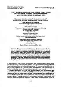
Fig. 2. Linear (s = 0, dotted line) and piecewise linear (s* = 0, solid line)sliding surfaces.

4.1. A novel FSMC methodology Consider system (1) and define the following variable: e + λe if  s* ( x ) =  e + λe H ⋅ sign(e) if

e < eH e ≥ eH

(13)

where the sliding constant λ and the design parameter eH are strictly positive. Now, consider the modified piecewise linear sliding surface (see Fig. 2): s*(x) = 0.

(14)

Hence, according to (13) and (14), the phase plane may be divided into two main zones. First, a region where |e| < eH (e.g. point A in Fig. 2) and the original and modified sliding surface overlap, with s*(x) = s(x) representing the vertical distance from such a surface. Second, a region containing the points in which |e| ≥ eH, where the two sliding lines and the vertical distances from such manifolds differ, i.e., s*(x) ≠ s(x). In particular, in the latter case we distinguish the following seven regions in the phase plane (Fig. 2): Zone 1: points with |e| < eH, s = s* (e.g. A in Fig. 2); Zone 2: points with |e| ≥ eH, |s*| ≤ |s| and s, s* ≥ 0 (e.g. B in Fig. 2);

Zone 3: points with |e| ≥ eH, |s*| ≤ |s| and s, s* ≤ 0 (e.g. C in Fig. 2); Zone 4: points with |e| ≥ eH, |s*| ≥ |s| and s, s* ≤ 0 (e.g. D in Fig 2); Zone 5: points with |e| ≥ eH, |s*| ≥ |s| and s, s* ≥ 0 (e.g. E in Fig 2); Zone 6: points with |e| ≥ eH and s* ≥ 0, s ≤ 0 (e.g. F in Fig. 2); Zone 7: points with |e| ≥ eH and s* ≤ 0, s ≥ 0 (e.g. G in Fig. 2). Now, consider system (1) with a FSMC law of type  λ) ) , u = b −1 (x) ⋅ ( uˆ * + u *fuzz(e, e,

(15)

where a discontinuous equivalent control is defined as follows  if x1d + λe) −(f (x) −  uˆ * =   − − (f (x) x1d ) if 

e < eH e ≥ eH

(16)

and the fuzzy contribution in (15) is identified by the term  λ ) = u* fuzz(s* (x)) u*fuzz(e, e, = −K fuzz (s* (x)) ⋅ sign(s* (x)).

(17)

In the sequel the FSMC rule table and design pa-

Asian Journal of Control, Vol. 5, No. 4, December 2003

532

rameters described in section 3 are maintained, with the substitution of s with s* and ufuzz with u*fuzz. In the following we show that system (1) is stable under the control law (15)-(16)-(17), i.e., the tracking error converges to zero in a finite time and the surface s*(x) = 0 is attractive for the closed-loop system. Proposition 1. The sliding line (14) is attractive for the state trajectory of system (1) under the FSMC with piecewise linear sliding manifold (15)-(16)-(17). Proof. Consider the Lyapunov function V=

1 *2 s (x). 2

=  x1d − λe − K fuzz (s* (x)) ⋅ sign(s* (x)) + d.

(19)

(20)

Hence, for all points x(t) such that |e| < eH, by (18) and (20) we get:  = s* (x) ⋅ s* (x) = s* (x) ⋅ (e  + λe) V = − K fuzz (s* (x)) ⋅ s* (x) + d ⋅ s* (x) ≤ −η* s* ( x)

(21)

where η* is a strictly positive design constant such that K*fuzzmax ≥ η* + D, K*fuzzmax being the upper bound of Kfuzz(s*(x)). On the other hand, for all the points x(t) such that |e| ≥ eH, by (13) we have s* (x) = ë. Now, reasoning as above, by (15)-(16)-(17) we get: e = − K fuzz (s* (x)) ⋅ sign(s* (x)) + d.

s* (x(t = 0)) η*

.

(23)

Proof. Let us call treach the time required to hit the attractive piecewise linear switching manifold (14). Assume for instance s*(t = 0) > 0. Integrating the modified sliding condition (21) between t = 0 and t = treach leads to: s* (t = t reach )

∫

sign(s* )ds* ≤ −η* ⋅

s* (t = 0)

t = t reach

∫

dt,

(24)

t =0

hence s* (t = t reach ) − s* (t = 0) ≤ −η* ⋅ (t reach − 0)

(25)

and trivial transformations lead to (23). The same result may be shown for s*(t = 0) < 0.

Therefore, we have: e = −λe − K fuzz (s* (x)) ⋅ sign(s* ( x)) + d.

t reach ≤

(18)

By (1), (15), (16) and (17), for all the operating points x(t) such that |e| < eH it holds: x 2 = f (x) + b( x) ⋅ u + d

(15)-(16)-(17). If the initial state is such that x1(t = 0) ≠ x1d(t = 0) and the system trajectory is off the piecewise linear sliding line (14), then the surface s*(x) = 0 will be reached in a finite time treach such that:

(22)

Hence, for all points x(t) such that |e| ≥ eH, it holds:  = s* (x) ⋅ s* (x) = s* (x) ⋅ e V = − K fuzz (s* (x)) ⋅ s* (x) + d ⋅ s* (x) ≤ −η* s* ( x) and we get the modified sliding condition (21) again.  is negative definite in the piecewise Therefore, V linear switching manifold, and the modified sliding line (14) is attractive for the FSMC (15)-(16)-(17). In particular, the modified sliding condition (21) guarantees reaching of the sliding line in a finite time. „ Proposition 2. Consider system (1) under the FSMC

A comparison of (23) with (8) shows that for an initial state in zone 1 in Fig. 2, such that s*(x) = s(x), the reaching time upper bound equals the one obtained with the classical sliding surface (2), under the hypothesis that the corresponding FSMCs share the same design structure and parameters. On the other hand, it is worth noting that if the initial state lies in a region different from zone 1 of the phase plane (see Fig. 2), then |s*(x)| ≠ |s(x)| and comparison of the reaching time upper bounds (23) and (8) depends on the choice of the design variables η and η* in the corresponding FSMCs. We have proven that after a reaching phase of finite duration the system trajectory hits the modified sliding surface (14). Now, to prove that (1) is stable under (15)-(16)-(17), we demonstrate that once the system enters the sliding mode it keeps sliding along the switching manifold to the origin (0, 0) of the phase plane, hence tracking is achieved. „ Proposition 3. Once the system (1) under (15)-(16)-(17) hits the piecewise linear switching manifold (14), the system trajectory converges to the origin of the phase plane. Proof. Let x(t = 0) be the initial state on the switching line (14). Hence, s*(x(t = 0)) = 0. Again, consider two possible circumstances. If x(t = 0) is such that |e| < eH, then s*(x(t = 0)) ≡ s(x(t = 0)) = 0 and integrating (2) leads to [21]: e(t) = e(t = 0)e−λt,

(26)

M. Dotoli: Fuzzy Sliding Mode Control with Piecewise Linear Switching Manifold

hence, the system trajectory converges to the origin with a time constant 1/λ. On the other hand, if x(t = 0) is such that |e| ≥ eH, and s*(x(t = 0)) = 0, by (13) it holds: e = −λeH ⋅ sign(e(t = 0)).

(27)

By integrating (27) between t = 0 and t such that |e| ≥ eH, we get: e(t) = e(t = 0) – λeH ⋅ sign(e(t = 0)) ⋅ t

(28)

or, equivalently, |e(t)| = |e(t = 0)| − λeH ⋅ t.

(29)

Hence, |e(t)| decreases until the trajectory enters zone 1 in figure 2 and (26) holds. We remark that the larger the factor λ·eH, the faster the reduction of the error magnitude. „ The proposed FSMC with piecewise linear switching manifold guarantees tracking of the desired trajectory and represents an alternative to the traditional FSMC discussed in section 3. Moreover, it is worth noting that in numerous applications employing the proposed FSMC with a proper choice of eH reduces the initial sliding variable magnitude with respect to the corresponding one obtained with a classical FSMC. It is reasonable to suppose that, if eH has been properly selected, the initial operating point belongs to zones 2 or 3 in Fig. 2. In particular, it often occurs that such an initial state is located on  = 0) = 0 . This the horizontal Cartesian axis, such that e(t corresponds to x2(t = 0) = x2d(t = 0), which is often the case (e.g. if x2 represents the plant speed, x2d(t) = 0 is desired and the initial velocity is equal to zero). If the initial operating point lies in zones 2 or 3 in Fig. 2, then |s*(x)| ≤ |s(x)| holds. Now, consider a modified FSMC differing from the one defined in the previous section only with regard to the input s*(x) as a replacement of s(x), while the rule table is the same. Hence, the fuzzy contribution to the control action is smaller than the corresponding one required when s(x) is the input to the FSMC. Summing up, a proper selection of eH results in an initial state in zones 2-3 such that |e| ≥ eH and a suitable value of K*fuzzmax forces the trajectory to hit the sliding mode in a finite time with an upper bound (23) and a reduced control action. In the following we discuss such a feature of the proposed FSMC with respect to the occurrence of saturation in the control input. 4.2 Comparison of the proposed FSMC with classical FSMC under saturation effects Although in real systems the control input is typi-

533

cally constrained by saturation effects, analyses of VSC techniques taking into account a saturated input are rare in the literature. In this sub-section we discuss the saturation effect occurring when the actuator range is limited with respect to the control action required by operation of a pure SMC or FSMC. If the actuator saturates, implementing a classical SMC (4) or FSMC (11) results in the following control law: u  u = sat  i  ⋅ U, U

(30)

where u and ui represent the actual and ideal control law respectively, U is the maximum available control magnitude and (10) holds. Consider an ideal FSMC: u i = b −1 (x) ⋅ (uˆ − K fuzz (s(x)) ⋅ sign(s(x))),

(31)

where (5) holds. The following discussion is detailed for FSMC, nevertheless we remark that the same results hold for pure SMC if we consider K as a replacement for Kfuzz in (31). Now, suppose that saturation occurs at a time instant t. By (30) it holds: u(t) = ±U,

(32)

ui(t) = ±U ± ∆(x(t)),

(33)

where ∆(x(t)) is the absolute value of the residual control action, depending on the actual system state at the time instant t. Hence, by (33) we may re-write (32) as follows: u = ui – sign(ui) ⋅ ∆(x)

(34)

where we neglected the time dependencies for sake of simplicity. Now, by derivation of (2) and taking into account the system dynamics (1) we get:  x) = f (x) + b(x) ⋅ u + d(x) −   s( x1d + λe.

(35)

Hence, by substitution of (34), (31) and (5) in (35) it holds:  x) = − K fuzz (s(x)) ⋅ sign(s(x)) + d(x) s( − b(x) ⋅ ∆ (x) ⋅ sign(u i ).

(36)

Now, consider the derivative of the Lyapunov function (3):  = s(x)s(  x) = − s(x) ⋅ (K fuzz (s(x)) − d(x) ⋅ sign(s(x)) V + b(x) ⋅ ∆(x) ⋅ sign(s(x) ⋅ u i )).

(37)

 is negative definite in the sliding surHence, V

Asian Journal of Control, Vol. 5, No. 4, December 2003

534

face (2) if it holds: K fuzz (s(x)) − d(x) ⋅ sign(s(x)) + b(x) ⋅ ∆ (x) ⋅ sign(s(x) ⋅ u i ) > 0.

∆* ( x ) < (38)

We remark that by design of the FSMC the sliding condition (7) holds, i.e.: K fuzz (s(x)) − d(x)sign(s(x)) ≥ η > 0.

(39)

 remains negative definite in the sliding Hence, V surface under (34) if it holds:

η > − b(x) ⋅ ∆(x) ⋅ sign(s(x) ⋅ u i ) = − b(x) ⋅ ∆ (x) ⋅ sign(s(x) ⋅ b( x) ⋅ u i ).

(40)

Now, if sign(s(x) · b(x) · ui) ≥ 0, then (40) is true. On the other hand, if sign(s(x) · b(x) · ui) = −1 a sufficient condition for (40) to hold is ∆ (x)