Fuzzy Spatial Data Types for Spatial Uncertainty

Fuzzy Spatial Data Types for Spatial Uncertainty Management in Databases Markus Schneider University of Florida Department of Computer & Information Science & Engineering Gainesville, FL 32611, USA [email protected]

Abstract Spatial database systems and geographical information systems are currently only able to support geographical applications that deal with crisp spatial objects, that is, objects whose extent, shape, and boundary are precisely determined. Examples are land parcels, school districts, and state territories. However, many new, emerging applications are interested in modeling and processing geographic data that are inherently characterized by spatial vagueness or spatial indeterminacy. This requires novel concepts due to the lack of adequate approaches and systems. In this chapter, we focus on an important kind of spatial vagueness called spatial fuzziness. Spatial fuzziness captures the property of many spatial objects in reality which do not have sharp boundaries and interiors or whose boundaries and interiors cannot be precisely determined. We will designate this kind of entities as fuzzy spatial objects. Examples are air polluted areas, temperature zones, and lakes. We propose an abstract, formal, and conceptual model of so-called fuzzy spatial data types (that is, a fuzzy spatial algebra) introducing fuzzy points, fuzzy lines, and fuzzy regions in the two-dimensional Euclidean space. This chapter provides a definition of their structure and semantics, which is supposed to serve as a specification of their implementation. Further, we introduce fuzzy spatial set operations like fuzzy union, fuzzy intersection, and fuzzy difference as well as fuzzy topological predicates as they are useful in fuzzy spatial joins and fuzzy spatial selections. We also sketch implementation strategies for the whole type system and show their integration into databases. An outlook to future research challenges rounds off the chapter.

INTRODUCTION Spatial database systems (SDBS) are full-fledged database systems which, in addition to the functionality of standard database systems for alphanumeric data, provide special support for the storage, retrieval, management, and querying of spatial data, that is, objects in space. In particular, SDBS are used as data management components of Geographical Information Systems (GIS). For modeling and storing spatial data, special data types called spatial data types (see Schneider (1997) for an introduction and survey) have been designed. The most established spatial data types are called point, line, and region. We speak of spatial objects as instances of these data types. So far, these data types are only able to represent spatial data whose extent and hence border is precisely determined and homogeneous. Spatial phenomena are represented by sharply described points with exactly known coordinates, lines linking a series of exactly known points, and regions bounded by exactly defined lines called boundaries. The properties of the space at the points, along the lines, or within the regions are given by attributes whose values are assumed to be constant over the total extent of the objects. Well known examples are especially man-made spatial objects representing engineered artifacts like highways, houses, or bridges and some predominantly immaterial spatial objects exerting social control

like countries, districts, and land parcels with their political, administrative, and cadastral boundaries. We denote this kind of entities as crisp or determinate spatial objects. In the last years, geographical applications and GIS have shown increasing interest in data models for spatial data that are characterized by the inherent feature of spatial vagueness or spatial indeterminacy (Burrough & Frank, 1996). The reason for this interest is that the current mapping of spatial phenomena of the real world to exclusively crisp spatial objects has turned out to be an inadequate abstraction process for many kinds of spatial data. Consequently, applications based on indeterminate spatial data are not covered by current GIS and SDBS. In this chapter we focus on a special kind of spatial vagueness called spatial fuzziness. Fuzziness captures the property of many spatial objects in reality which do not have sharp boundaries and interiors or whose boundaries and interiors cannot be precisely determined. Examples are natural, social, or cultural phenomena like land features with continuously changing properties (such as population density, soil quality, vegetation, pollution, temperature, air pressure), oceans, deserts, English speaking areas, or mountains and valleys. The transition between a valley and a mountain usually cannot be exactly ascertained so that the two spatial objects “valley” and “mountain” cannot be precisely separated and defined in a crisp way. We will designate this kind of entities as fuzzy or indeterminate spatial objects. This chapter delineates ongoing research on fuzzy spatial objects in databases and pursues several goals. First, we present an abstract, formal, and conceptual object model providing fuzzy spatial data types for fuzzy points, fuzzy lines, and fuzzy regions in the two-dimensional Euclidean space. Second, we introduce some fuzzy spatial operations and a concept of fuzzy topological predicates. The entire effort is supposed to lead to a formal specification of a fuzzy spatial algebra. Fuzzy set theory (Zadeh, 1965; Buckley & Eslami, 2002) and fuzzy topology (Liu & Luo, 1997) are the formal framework of the algebra design. Third, we show how fuzzy spatial data types, operations, and topological predicates can be integrated into database systems and their query languages and be used as attribute types in database schemas. Fourth, we provide some implementation ideas. Section “Related Work” explains different aspects of spatial vagueness and presents related work. Section “Abstract Definition of Fuzzy Spatial Data Types” introduces some basic concepts and notations of fuzzy set theory and fuzzy topology, as far as they are used in this chapter, and formally defines the data types for fuzzy points, fuzzy lines, and fuzzy regions. In Section “Fuzzy Topological Predicates”, we introduce a concept of fuzzy topological predicates describing the relative position of fuzzy spatial objects towards each other. Section “Database Integration of and Querying with Fuzzy Topological Predicates” deals with the integration of the fuzzy spatial algebra into databases by leveraging the concept of abstract data types and demonstrates the use of fuzzy topological predicates in an SQL-like spatial query language. Section “Conclusions and Future Work” draws some conclusions and considers future work.

RELATED WORK The first subsection discusses the nature of imperfect spatial data and gives an overview of the general methods for modeling them. The second subsection deals with spatial fuzziness which is a special kind of spatial imperfection and the topic of this chapter.

SPATIAL IMPERFECTION For a long time, the treatment of imperfect data has found large research interest in computer science. In the database field, the emphasis has been on investigating the impact of imperfect data (Parsons, 1996) on data modeling, classical database functions like storage, indexing, retrieval, update, and query functionalities as well as the entire database system architecture. In this chapter, we deal with the imperfection of spatial data. More precisely, we focus on a special kind of spatial imperfection, which we call spatial vagueness. Spatial vagueness manifests itself in indetermi2

nate boundaries and interiors of spatial objects. In the real world, there are essentially two categories of indeterminate boundaries: sharp boundaries whose position and shape are unknown or cannot be measured precisely, and boundaries which are not well-defined or which are useless (for example, between a mountain and a valley) and where essentially the topological relationship between spatial objects is of interest. Spatial objects with indeterminate boundaries are difficult to model and implement and are so far not supported in spatial databases systems. According to the two categories of boundaries, mainly two kinds of spatial vagueness can be identified: spatial uncertainty and spatial fuzziness. Spatial uncertainty is traditionally equated with randomness and chance occurrence and relates either to a lack of knowledge about the position and shape of an object with an existing, real boundary (positional uncertainty) or to the inability of measuring such an object precisely (measurement uncertainty). Spatial fuzziness is an intrinsic feature of an object itself and describes the vagueness of an object which certainly has an extent but which inherently cannot or does not have a precisely definable boundary. The subject of modeling spatial vagueness has so far been predominantly treated by geographers and GIS experts but rather neglected by computer scientists. A main reason is that the treatment of spatial objects with indeterminate boundaries is especially problematic for the computer scientist who is confronted with the difficulties how to model such objects in his database system so that they correspond to the user’s intuition, how to finitely represent them in a computer format, how to develop spatial algorithms and index structures for them, and how to draw them. He is accustomed to the abstraction process of simplifying spatial phenomena of the real world through the concepts of conventional binary logic, reduction of dimension, and cartographic generalization to precisely defined, simply structured, and sharply bounded objects of Euclidean geometry like points, lines, and regions. At least four alternatives are proposed as general design methods: exact object models, probabilistic models, rough set-based models, and fuzzy set-based models. Exact object models transfer data models, type systems, and concepts for spatial objects with sharp boundaries to objects with unclear boundaries. A benefit of this approach is that existing definitions, techniques, data structures, algorithms, etc. need not be redeveloped but only modified and extended, or simply used. The approaches in (Clementini & Di Felice, 1996a; Cohn & Gotts, 1996; Schneider, 1996) propose a zone concept. The central idea is to consider determined zones surrounding the indeterminate boundaries of a region (broad boundaries) and expressing its minimal and maximal extent. The zones serve as a description and separation of the space that certainly belongs to the region, that perhaps belongs to the region, and that is certainly outside. The approaches in (Erwig & Schneider, 1997; Pauly & Schneider, 2004) generalize these concepts and introduce vague spatial data types for vague points, vague lines, and vague regions. A vague spatial object is modeled as a pair of two meeting or disjoint crisp spatial objects. For example, a vague region is given as a pair of two meeting or disjoint crisp regions. The first object is the kernel part and models the part that definitely belongs to the vague spatial object. The second object is the conjecture part from which we can only assume that it or parts of it belong to the vague object. Predicates on vague spatial objects are based on a three-valued logic with the values true, false, and maybe (Pauly & Schneider, 2005; Pauly & Schneider, 2006). Probabilistic models are able to represent positional and measurement uncertainty. Their basis is probability theory which defines the grade of membership of an entity in a set by a statistically defined probability function and deals with the expectation of a future event, based on something known now. As an example of a large amount of literature, Blakemore (1984) describes the uncertainty in the position of a line using a band of width ε. Rough set-based models are based on rough set theory (Pawlak, 1982) and model vague spatial objects by a lower and an upper spatial approximation. As an example, Beaubouef, Ladner, and Petry (2004) show how rough sets can be used for spatial data modeling in a data mining environment. Fuzzy set-based models are based on fuzzy set theory (Zadeh, 1965). It describes the admission of the possibility (given by a so-called membership function) that an individual is a member of a set or that a given statement is true. Hence, the vagueness represented by fuzziness is not the uncertainty of expectation. It is 3

the vagueness resulting from the imprecision of meaning of a concept. We describe some relevant literature in the next subsection.

SPATIAL FUZZINESS Fuzzy databases have established themselves as an important branch in the database field to handle fuzzy data as a particular kind of imperfect data. This has led to a large volume of literature in this field. Examples of books on fuzzy databases that cover modeling, design, and implementation issues are (Petry, 1996; Galindo, Urrutia, & Piattini, 2006). The books of Yazici and George (1999) and Ma (2005) emphasize the aspect of fuzzy database modeling. The deployment of fuzzy set theory and fuzzy logic for spatial applications and spatial analysis methods has found large attraction in the geoscience and GIS communities and also led to a large amount of literature on fuzzy approaches in the GIS domain. A spatial concept is vague or fuzzy if locations exist that cannot be completely associated with the concept or with its complement. For example, when mapping vegetation, it is difficult to determine whether a certain location belongs to one vegetation class or to another. Examples from the geosciences that exhibit transition zones instead of sharp boundaries and that have been modeled with fuzzy concepts are geomorphological units (Burrough, van Gaans, & Macmillan, 2000), soil types and boundaries (De Gruijter, Walvoort, & Vangaans, 1997; Lagacherie, Andrieux, & Bouzigues, 1996), landscape objects (Cheng, Molenaar, & Lin, 2001), forest types (Brown, D.G., 1998), soil pollution classes in environmental applications (Hendricks Franssen, van Eijnsbergen, & Stein, 1997), and hydrological studies (Bog`ardi, B´ardossy, & Duckstein, 1990). Burrough (1996) introduces fuzzy geographical objects for modeling natural objects with indeterminate boundaries. Dutta (1989, 1991) as well as Kollias and Voliotis (1991) deal with qualitative spatial and temporal reasoning using fuzzy logic. Edwards (1994) and Wang and Hall (1996) deal with fuzzy representations of geographical boundaries in GIS. Usery (1996) defines concepts like core and boundary of a fuzzy region and gives examples of membership functions for modeling fuzzy regions. Wang (1994) presents a fuzzy query approach in order to introduce more natural language expressions into GIS user interfaces. Wang, Hall, and Subaryono (1990) propose a fuzzy relational data model for geographic information; each tuple is annotated with a membership value. Another chapter in this book written by Xex´eo presents a tool for fuzzy reasoning and querying and its application into a GIS for modeling a malaria surveillance system in Brazil. The references mentioned so far demonstrate the usefulness of fuzzy concepts in geoscience applications from a modeling standpoint. However, they do not deal with the issue of representing, storing, retrieving, and querying fuzzy spatial objects in fuzzy spatial databases. Increasingly, there is interest in pursuing these goals. Altman (1994) presents fuzzy set theoretic approaches for handling imprecision in spatial analysis and introduces fuzzy regions as a binary relation on the domain of N2 (N denotes the set of natural numbers). Distance and directional metrics on fuzzy regions demonstrate their possible use in qualitative spatial analysis. Schneider (1999) provides the foundation of fuzzy spatial data types for fuzzy points, fuzzy lines, and fuzzy regions and also specifies fuzzy spatial operations like fuzzy spatial union, fuzzy spatial intersection, and fuzzy spatial difference. The author presents an abstract specification in which fuzzy spatial objects are defined as special fuzzy sets from R2 . Dilo, de By, & Stein (2007) introduce a similar type system of vague spatial data types with a more comprehensive set of operations. Instead of the term “fuzzy”, they use the term “vague”. As an extension, they specify the concept of a vague partition. Schneider (2003) proposes a conceptual model and an implementation model of fuzzy spatial objects that are not defined on the Euclidean plane but on a discrete geometric domain called grid partition; it takes into account finiteprecision number systems available in computers. Membership values are assigned to the points, edges, and cells as elements of the grid partition; fuzzy objects are built from these grid elements. Schneider (2000) presents metric operations on fuzzy spatial objects like the area of a fuzzy region or the length of a fuzzy line. Different models of fuzzy topological predicates, which characterize the relative position of two fuzzy

4

spatial objects towards each other, are discussed in (Petry et al., 2002; Schneider, 2001a, 2001b; Shi & Guo, 1999; Tang X., & Kainz W., 2002; Zhan, 1997, 1998).

ABSTRACT DEFINITION OF FUZZY SPATIAL DATA TYPES For crisp, two-dimensional spatial data, spatial data types for points, lines, and regions (Schneider, 1997) have found a broad consensus in the spatial database and GIS communities as appropriate two-dimensional abstractions of real world objects. In this section, we give formal definitions of their fuzzy counterparts. The definitions are abstract, that is, based on fuzzy set theory and fuzzy topology. They focus on the determination of the essential features of fuzzy spatial objects without taking into account any data representation issues and algorithmic aspects in computer systems and are intended as a specification for a possible implementation. Therefore, we can use concepts like infinite sets, relations, and functions in our definitions. Finiteness only plays a role when we specify the number of components of an object. Since there will never be a chance to represent an object with an infinite number of components in a computer, we require this number to be finite. On the other hand, to represent the infinite point set of an object component by a finite representation is usually possible. The first subsection introduces some basic concepts and notations of fuzzy set theory and fuzzy topology as far as they are used in this chapter. The subsequent three subsections formally define the data types for fuzzy points, fuzzy lines, and fuzzy regions respectively.

FUZZY SETS AND FUZZY TOPOLOGY Crisp spatial data types (for example, (Clementini & Di Felice, 1996b; Schneider, 1997; Schneider & Behr, 2006)) for points, lines, and regions have been formally defined on the basis of point sets and point set topology (Gaal, 1964). Our goal is to leverage their fuzzy counterparts for a definition of fuzzy spatial data types. In this section, we summarize some needed basic concepts and notations of fuzzy set theory and fuzzy topology. Fuzzy set theory (Zadeh, 1965; Buckley & Eslami, 2002) is an extension and generalization of Boolean set theory. Let X be a classical (crisp) set of objects, called the universe (of discourse). Membership in a classical subset A of X can then be described by the characteristic function χA : X → {0, 1} such that for all x ∈ X holds: ( 1 if, and only if, x ∈ A χA (x) = 0 if, and only if, x ∈ /A This function, which discriminates sharply between members and non-members of a set, can be generalized such that all elements of X are mapped to the real interval [0,1] indicating the degree of membership of these elements in the set in question. Hence, fuzzy set theory permits an element to have partial membership in a fuzzy set and/or multiple membership in several, different fuzzy sets. Larger values designate higher grades of set membership. Let X again be the universe. Then µA˜ : X → [0, 1] ˜ and the set is called the membership function of A, A˜ = {(x, µA˜ (x)) | x ∈ X} ˜ Those is called a fuzzy set in X. All elements of X receive a valuation with respect to their membership in A. elements x ∈ X that in the classical sense do not belong to A˜ get the membership value µA˜ (x) = 0; elements x ∈ X that completely belong to A˜ get the membership value µA˜ (x) = 1. 5

Next, we extend the set inclusion as well as the basic crisp set operations to fuzzy sets. We will comply with the definitions in Zadeh (1965). Let A˜ and B˜ be fuzzy sets in X. Then (i) ¬A˜ = {(x, µ¬A˜ (x)) | x ∈ X, µ¬A˜ (x) = 1 − µA˜ (x)} ˜ (ii) A ⊆ B˜ ⇔ ∀ x ∈ X : µA˜ (x) ≤ µB˜ (x) (iii) A˜ ∩ B˜ = {(x, µA∩ ˜ B˜ (x)) | x ∈ X ∧ µA∩ ˜ B˜ (x) = min(µA˜ (x), µB˜ (x))} (iv) A˜ ∪ B˜ = {(x, µA∪ (x)) | x ∈ X ∧ µ ˜ B˜ ˜ B˜ (x) = max(µA˜ (x), µB˜ (x))} A∪ ˜ ˜ ˜ ˜ (v) A − B = A ∩ ¬B An α-cut or α-level set of a fuzzy set A˜ for a specified value α is the crisp set A≥α = {x ∈ X | µA˜ (x) ≥ α ∧ 0 ≤ α ≤ 1} A strict α-cut or strict α-level set of a fuzzy set A˜ for a specified value α is the crisp set A>α = {x ∈ X | µA˜ (x) > α ∧ 0 ≤ α < 1} ˜ that is, supp(A) ˜ = A>0 . The α-cut for α = 1 is The strict α-cut for α = 0 is called the support of A, ≥1 ˜ that is, core(A) ˜ = A . For a fuzzy set A˜ and α, β ∈ [0, 1] holds called the core of A, (i) X = A≥0 (ii) α < β ⇒ A≥α ⊇ A≥β The set of all levels α ∈ [0, 1] that represent distinct α-cuts of a given fuzzy set A˜ is called the level set ˜ ΛA˜ of A: ΛA˜ = {α ∈ [0, 1] | ∃ x ∈ X : µA˜ (x) = α} Fuzzy (point set) topology (Chang, 1968; Liu & Luo, 1997) is a straightforward extension and generalization of ordinary point set topology and allows one to distinguish specific topological structures of a fuzzy set like its closure or interior. For a non-empty, crisp set X, let [0, 1]X = { f | f : X → [0, 1]} be the set of all mappings from X to [0, 1]. Let 1X be the function that corresponds to the whole set X, and 0X be the function that corresponds to the empty set ∅. A fuzzy topology on X is a family T ⊆ [0, 1]X of fuzzy sets satisfying the following conditions: (i) 1X ∈ T , 0X ∈ T (ii) A˜ ∈ T , B˜ ∈ T ⇒ A˜ ∩ B˜ ∈ T S ˜ ∈T (iii) S ⊆ T ⇒ A∈ ˜ SA The pair (X, T ) is said to be a fuzzy topological space. The elements of T are called open fuzzy sets1 . The family T 0 of all closed fuzzy sets2 in a fuzzy topological space (X, T ) is given by T 0 = {¬A˜ | A˜ ∈ T } The closure of a fuzzy set A˜ in a fuzzy topological space (X, T ) is the smallest closed fuzzy set contain˜ that is, ing A, ˜ = T {B˜ | B˜ ∈ T 0 ∧ A˜ ⊆ B} ˜ clT (A) The interior of a fuzzy set A˜ in a fuzzy topological space (X, T ) is the largest open fuzzy set contained ˜ in A, that is, ˜ = S {B˜ | B˜ ∈ T ∧ B˜ ⊆ A} ˜ intT (A) We obtain an example of a fuzzy topological space if we equate X with the Euclidean plane R2 . The fuzzy topological space (R2 , T ) is just of interest in this chapter. 1 Intuitively

speaking, a (crisp or fuzzy) set U is open if you can “wiggle” or “change” any point x in U by a small amount in any direction and still be inside U. 2 A (crisp or fuzzy) closed set contains its own boundary. Intuitively speaking, if you are “outside” a closed set and you “wiggle” a little bit, you will stay outside the set. The reason is that the complement of a closed set is open.

6

FUZZY POINTS The goal of this subsection is to design a concept of a fuzzy point object and to introduce a corresponding fuzzy spatial data type fpoint for this class of objects. First, we informally discuss some features of fuzzy points and compare them to crisp points. Then, we give their formal definition. WHAT ARE FUZZY POINTS? Points are the simplest geometric abstraction. They are the atoms, that is, the elements, of the Euclidean space R2 and form the basis of the point set paradigm. Each element of a crisp point set X of R2 belongs definitely and totally to this set. For each point of R2 , we can definitely say whether it belongs to X or not. A crisp point object, as it has been defined, for example, in (Schneider, 1997; Schneider & Behr, 2006), includes a finite set of points in order to ensure the closure of set operations. In the fuzzy domain, a fuzzy point set X˜ also represents a subset of R2 but each point of X˜ only has a certain partial membership in this set. It can also partially belong to another fuzzy set, that is, multiple set membership is possible. For example, if we consider an air-polluted area (which is a fuzzy region), then each point of this area is fuzzy since the concentration of air pollution at this point is not 100 percent. That is, the degree of membership of this fuzzy point in the air-polluted area is less than 1 and larger than 0. Fuzzy points can also arise as the result of two fuzzy lines. FORMAL DEFINITION OF FUZZY POINTS We now provide a formal definition of fuzzy points. We also show that the definition of a corresponding fuzzy spatial data type is not necessarily straightforward and that instead, due to the feature of spatial vagueness, several options can exist. We present here two meaningful definitions of fuzzy points that can be used as a foundation for a definition of the type fpoint. The first definition views a fuzzy point as a point in the two-dimensional Euclidean space with a membership value greater than 0, since 0 documents the non-existence of a point. A fuzzy point p˜ at (a, b) in R2 , written p(a, ˜ b), is a fuzzy singleton in R2 defined by ( m if (x, y) = (a, b) µ p(a,b) (x, y) = ˜ 0 otherwise with 0 < m ≤ 1. Point p˜ is said to have support (a, b) and value m. Let Pf be the set of all fuzzy points. Pf is a proper superset of Pc , the set of all crisp points in R2 . For p˜ = p = (a, b) ∈ Pc , we obtain µ p(a,b) (x, y) = ˜ χ p (x, y) = 1, if (x, y) = (a, b), and 0 otherwise. The second definition uses a membership function that returns the degree of proximity of a point to a reference point p. ˜ That is, we consider that the point (x, y) is “approximately (a, b)” or “about (a, b)” to the degree µ p(a,b) (x, y). A fuzzy point p(a, ˜ b) is then generally defined by ˜ (i) µ p(a,b) is upper semicontinuous3 ˜ (ii) µ p(a,b) (x, y) = 1 if, and only if, (x, y) = (a, b) ˜ (iii) ∀ 0 ≤ α ≤ 1 : p˜≥α is a convex4 subset of R2 The “distance-based” membership function 3 A function f : X → R is upper semicontinuous :⇔ ∀ r ∈ R : {x | f (x) < r} is open. (The notation “:⇔” means “is defined as being equivalent”.) 4 A set X ⊆ R2 is called convex :⇔ ∀ p, q ∈ R2 ∀ λ ∈ R+ with 0 < λ < 1 : r = λ p + (1 − λ) q ∈ X (p, q, and r are here regarded as vectors).

7

2 +(y−b)2 )

µ p(a,b) (x, y) = c−λ ((x−a) ˜

with c ∈ R+ , c > 1, and λ > 0 illustrates this definition. The degree of proximity decreases as (x, y) moves further away from (a, b). It reaches 1 if (x, y) = (a, b). Unfortunately, this membership function with unbounded support is difficult to represent. Alternatively, we can employ the following, restricted but more practical function which defines a circle around (a, b) with radius r ∈ R+ : √ ( (x−a)2 +(y−b)2 1− if (x − a)2 + (y − b)2 ≤ r2 r µ p(a,b) (x, y) = ˜ 0 otherwise Next, we define three geometric primitives on fuzzy points which are valid for both definitions of fuzzy points. Let p(a, ˜ b), q(c, ˜ d) ∈ Pf with a, b, c, d ∈ R. Then (i) p(a, ˜ b) = q(c, ˜ d) :⇔ a = c ∧ b = d ∧ µ p(a,b) = µq(c,d) ˜ ˜ (ii) p(a, ˜ b) 6= q(c, ˜ d) :⇔ ¬( p(a, ˜ b) = q(c, ˜ d)) (iii) p(a, ˜ b) and q(c, ˜ d) are disjoint :⇔ supp( p(a, ˜ b)) ∩ supp(q(c, ˜ d)) = ∅ In contrast to crisp points, for fuzzy points we also have a predicate for disjointedness. We are now able to define an object of the fuzzy spatial data type fpoint as a set of disjoint fuzzy points: fpoint = {Q ⊆ Pf | ∀ p, ˜ q˜ ∈ Q : p(a, ˜ b) and q(c, ˜ d) are disjoint ∧ Q is finite} Disjointedness of the single fuzzy points of a fuzzy point object is required since the membership degree of each single fuzzy point should be unique.

FUZZY LINES This subsection provides a concept of a fuzzy line object and introduces a corresponding fuzzy spatial data type fline. First, we informally discuss some features of fuzzy lines and compare them to crisp lines. Then, we give their formal definition. WHAT ARE FUZZY LINES? Lines are the one-dimensional, geometric abstraction for linear features like rivers, boundaries, and transportation routes. Each crisp line is a subset of the Euclidean plane R2 with particular properties. Each element of a single crisp line is a crisp point that definitely and totally belongs to the line. A crisp line object (see, for example, Schneider, 1997; Schneider & Behr, 2006) includes a finite set of blocks. Each block consists of a finite set of simple lines (curves) such that each pair of simple lines is either disjoint or meets in a common end point. Fuzzy lines are supposed to adopt the fundamental structure of crisp lines. That is, a fuzzy line X˜ has the same linear geometry as a crisp line and is hence a subset of R2 ; however, each point of X˜ may only ˜ For example, the pollution of a river can be represented by the line be to some degree a member of X. geometry of the river where each point represents the degree or concentration of pollution at that location. The concentration is larger than 0 for all points of the fuzzy line but usually different at different locations. FORMAL DEFINITION OF FUZZY LINES We now specify the fuzzy spatial data type fline for fuzzy lines. For that, we first introduce a simple fuzzy line as a continuous curve with smooth transitions of membership grades between neighboring points of the line (Figure 1(a)). We assume a total order on R2 which is given by the lexicographic order “ 2)}

i=1 li | m

i

i

An example of a fuzzy line object is given in Figure 1(b).

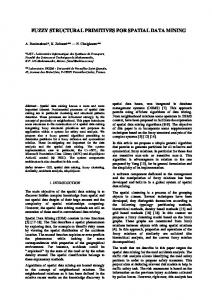
FUZZY REGIONS The aim of this subsection is to develop and formalize the concept of a fuzzy region and to introduce a corresponding fuzzy spatial data type fregion for them. First, we informally discuss some intrinsic features of fuzzy regions and compare them to classical crisp regions. Then, we provide their formal definition. Finally, we give some examples of possible membership functions for them. WHAT ARE FUZZY REGIONS? Research on spatial data modeling has so far focused on crisp or determinate spatial objects. The properties of crisp regions have been described in many publications. A very general definition defines a crisp region as a set of disjoint, connected areal components, called faces, possibly with disjoint holes (Clementini & Di Felice, 1996b; Schneider, 1997; Schneider & Behr, 2006) in the Euclidean space R2 . This model has the nice property that it is closed under (appropriately defined) geometric union, intersection, and difference operations. For example, if we intersect two crisp regions, the result is always a crisp region. The model also allows crisp regions to contain holes and islands within holes to any finite level. By analogy with the generalization of crisp sets to fuzzy sets, we strive for a generalization of crisp regions to fuzzy regions on the basis of the point set paradigm and fuzzy concepts. At the same time we would like to transfer the structural definition of crisp regions (that is, the component view) to fuzzy regions. Thus, the structure of a fuzzy region is supposed to be the same as for a crisp region but with the exception and generalization which amounts to a relaxation and hence greater flexibility of the strict belonging or non-belonging principle of a point in space to a specific region and which enables a partial membership of a point in a region. This is just what the term “fuzzy” means here. There are at least three possible, related interpretations for a point in a fuzzy region. First, this situation may be interpreted as the degree of belonging to which that point is inside or part of some areal feature. Consider the transition between a mountain and a valley and the problem to decide which points have to 10

Figure 2: Example of a fuzzy region consisting of two fuzzy faces as components. be assigned to the valley and which points to the mountain. Obviously, there is no strict boundary between them, and it seems to be more appropriate to model the transition by partial and multiple membership. Second, this situation may indicate the degree of compatibility of the individual point with the attribute or concept represented by the fuzzy region. An example are “warm areas” where we must decide for each point whether and to which grade it corresponds to the concept “warm”. Third, this situation may be viewed as the degree of concentration of some attribute associated with the fuzzy region at the particular point. An example is air pollution where we can assume the highest concentration at power stations, for instance, and lower concentrations with increasing distance from them. All these related interpretations give evidence of fuzziness. When dealing with crisp regions, the user usually does not employ point sets as a method to conceptualize space. The user rather thinks in terms of sharply determined boundaries enclosing and grouping areas with equal properties or attributes and separating different regions with different properties from each other; he or she has purely qualitative concepts in mind. This view changes when fuzzy regions come into play. Besides the qualitative aspect, in particular the quantitative aspect becomes important, and boundaries in most cases disappear (between a valley and a mountain there is no strict boundary!). The distribution of attribute values within a region and transitions between different regions may be smooth or continuous. This feature just characterizes fuzzy regions. There are a lot of spatial phenomena showing a smooth behavior. Application examples are air pollution, temperature zones, magnetic fields, storm intensity, and sun insolation. Figure 2 demonstrates a possible visualization of a fuzzy region object which could model the expansion of air pollution caused by (two nearby) power stations. The left image shows a radial expansion of the first power station where the degree of pollution concentrates in the center (darker locations) and decreases with increasing distance from the power station (brighter locations). The right image shows the distribution of air pollution of the second power station that is surrounded by high mountains to the north, the south, and the west. Hence, the pollution cannot escape in these directions and finds its way out of the valley in eastern direction. In both cases we can recognize the smooth transitions to the exterior. We call each connected component a fuzzy face. FORMAL DEFINITION OF FUZZY REGIONS Since our objective is to model two-dimensional fuzzy areal objects for spatial applications, we consider a fuzzy topology T on the Euclidean plane R2 . In this spatial context, we denote the elements of T as fuzzy point sets. The membership function for a fuzzy point set A˜ in the plane is then described by µA˜ : R2 → [0, 1]. From an application point of view, there are two observations that prevent a definition of a fuzzy region simply as a fuzzy point set. We will discuss them now in more detail and at the same time elaborate properties of fuzzy regions. Avoiding Geometric Anomalies: Regularization. The first observation refers to a necessary regularization of fuzzy point sets. The first reason for this measure is that fuzzy (as well as crisp) regions that actually appear in spatial applications in most cases cannot be just modeled as arbitrary point sets but have to be

11

Figure 3: Example of a fuzzy set that is not fuzzy region due to lower-dimensional, geometric anomalies like cuts, punctures, and dangling lines. represented as point sets that do not have “geometric anomalies” and that are in a certain sense regular. Geometric anomalies relate to isolated or dangling line or point features and missing lines and points in the form of cuts and punctures. Spatial phenomena with such degeneracies never appear as entities in reality. The second reason is that, from a data type point of view, we are interested in fuzzy spatial data types that satisfy closure properties for (appropriately defined) geometric union, intersection, and difference. We are, of course, confronted with the same problem in the crisp case where the problem can be avoided by the concept of regularity (Tilove, 1980; Schneider, 1997). It turns out to be useful to appropriately transfer this concept to the fuzzy case. Let A˜ be a fuzzy set of a fuzzy topological space (R2 , T ). Then ˜ A˜ is called a regular open fuzzy set if A˜ = intT (clT (A)) Whereas crisp regions are usually modeled as regular closed crisp sets, we will use regular open fuzzy sets due to their vagueness and their usual lack of boundaries. Regular open fuzzy sets avoid the aforementioned geometric anomalies, too. Since application examples show that fuzzy regions can also be partially bounded, we admit partial boundaries with a crisp or fuzzy character. For that purpose, we define the frontier of a fuzzy set as (The notation “:=” means “is defined as”.): ˜ − supp(intT (A))} ˜ ˜ := {((x, y), µA˜ (x, y)) | (x, y) ∈ supp(A) frontierT (A) ˜ − supp(intT (A)) ˜ determines the crisp locations of all fuzzy points of A˜ that are not The term supp(A) interior points. However, these locations do not necessarily all belong to the boundary of A˜ since A˜ has not been constrained so far. This is done in the following definition. A fuzzy set A˜ is called a spatially regular fuzzy set if, and only if, ˜ is a regular open fuzzy set (i) intT (A) ˜ ⊆ frontierT (clT (intT (A))) ˜ (ii) frontierT (A) ˜ (iii) frontierT (A) is a partition of n ∈ N connected boundary parts (fuzzy sets) Not every set A˜ is a spatially regular fuzzy set. Therefore, condition (i) ensures that the interior of A˜ is without any geometric anomalies. The other two conditions arrange for a correct (partial) boundary if ˜ is a regular it exists. Condition (ii) works as follows: On the right side of “⊆”, the set A˜ 0 = clT (intT (A)) ˜ closed fuzzy set, that is, the interior of A is complemented by its boundary without any geometric anomalies. Hence, the frontierT operator applied to A˜ 0 yields the boundary of A˜ 0 . The condition now requires that the frontier of A˜ is a subset of the frontier of A˜ 0 and does not contain other fuzzy points. Condition (iii) states that the frontier of A˜ has to consist of a finite number of connected pieces due to the “finite component assumption” explained before. Infinitely many boundary pieces cannot be represented in an implementation. ˜ = ∅ if A˜ is regular open. We will From the definition of frontierT , we can conclude that frontierT (A) base our definition of fuzzy regions on spatially regular fuzzy sets and define a regularization function reg f which associates the interior of a fuzzy set A˜ with its corresponding regular open fuzzy set and which restricts the partial boundary of A˜ (if it exists at all) to a part of the boundary of the corresponding regular ˜ closed fuzzy set of A: 12

˜ := intT (clT (A)) ˜ ∪ (frontierT (A) ˜ ∩ frontierT (clT˜ (intT (A)))) ˜ reg f (A) The different components of the regularization process work as follows: the interior operator intT eliminates dangling point and line features since their interior is empty. The closure operator clT removes cuts and punctures by appropriately adding points. Furthermore, the closure operator introduces a fuzzy boundary (similar to a crisp boundary in the ordinary point-set topological sense) separating the points of a closed set from its exterior. The operator frontierT supports the restriction of the boundary. The following statements about set operations on regular open fuzzy sets are given informally and without proof. The intersection of two regular open fuzzy sets is regular open. The union, difference, and complement of two regular open fuzzy sets are not necessarily regular open since they can produce anomalies. Correspondingly, this also holds for spatially regular fuzzy sets. Hence, we introduce regularized set ˜ B˜ be spatially regular fuzzy sets of operations on spatially regular fuzzy sets that preserve regularity. Let A, 2 a fuzzy topological space (R , T ), and let a−b ˙ = a − b for a ≥ b and a−b ˙ = 0 otherwise (a, b ∈ R+ 0 ). Then (i) (ii) (iii) (iv)

˜ A˜ ∪r B˜ := reg f (A˜ ∪ B) ˜ A˜ ∩r B˜ := reg f (A˜ ∩ B) ˜ ∧ µA− ˜ ˜ A −r B := reg f ({((x, y), µA− ˙ B˜ (x, y)}) ˜ r B˜ (x, y) | (x, y) ∈ supp(A) ˜ r B˜ (x, y) = µA˜ (x, y)−µ ˜ ¬r A˜ := reg f (¬A)

˜ since the right side of Note that we have changed the meaning of difference (i.e., A˜ −r B˜ 6= A˜ ∩r ¬B) the inequality is not meaningful in the spatial context. Regular open fuzzy sets, spatially regular fuzzy sets, and regularized set operations express a natural formalization of the desired closure properties of fuzzy geometric set operations. In the crisp case, this is taken for granted but mostly never fulfilled by spatial type systems, geometric algorithms, spatial database systems, and GIS. Whereas the subspace RCCS of regular closed crisp sets together with the crisp regular set operations “⊕” (geometric union) and “⊗” (geometric intersection) and the set-theoretic order relation “⊆” forms a Boolean lattice, this is not the case for SRFS denoting the subspace of spatially regular f uzzy sets. Here we obtain the (unproven but obvious) statement that SRFS together with the regularized set operations “∪r ” and “∩r ” and the fuzzy set-theoretic order relation “⊆” is a pseudo-complemented distributive lattice. This ˜ implies that (i) (SRFS, ⊆) is a partially ordered set (reflexivity, antisymmetry, transitivity), (ii) every pair A, ˜ (iii) (SRFS, ⊆) has B˜ of elements of SRFS has a least upper bound A˜ ∪r B˜ and a greatest lower bound A˜ ∩r B, 2 R 2 a maximal element 1 := {((x, y), µ(x, y)) | (x, y) ∈ R ∧ µ(x, y) = 1} (identity of “∩r ”) and a minimal 2 element 0R := {((x, y), µ(x, y)) | (x, y) ∈ R2 ∧ µ(x, y) = 0} (identity of “∪r ”), and (iv) algebraic laws like idempotence, commutativity, associativity, absorption, and distributivity hold for “∪r ” and “∩r ”. (SRFS, ⊆) is not a complementary lattice. Although the algebraic laws of involution and dualization hold, this is not true for the laws of complementarity. If we take the standard fuzzy set operations presented 2 in the Section “Fuzzy Sets and Fuzzy Topology” as a basis, the law of excluded middle A˜ ∪r ¬A˜ = 1R 2 and the law of contradiction A˜ ∩r ¬A˜ = 0R do not hold in general. This fact explains the term “pseudocomplemented” from above and is not a weakness of the model but only an indication of fuzziness. Modeling Smooth Attribute Changes: Continuous Membership Functions. The second observation is that, according to the application cases shown before, the mapping µA˜ itself may not be arbitrary but must take into account the intrinsic smoothness of fuzzy regions. This property can be modeled by the well known mathematical concept of continuity. Here, we employ the concept of a piecewise continuous function for modeling the smooth membership distribution in a single fuzzy face. A function is piecewise continuous if it is made of a finite number of continuous pieces. Hence, it has only a finite number of discontinuities (continuity gaps), and its left and right limits are defined at each discontinuity. The only possible kinds of discontinuities for a piecewise continuous function are removable and step discontinuities. A removable discontinuity represent a hole in the function graph. It can be repaired by filling in a single point. A step 13

discontinuity (also called semi-continuity) is a location in the function graph where the graph steps or jumps from one connected piece of the graph to another. Formally, it is a discontinuity for which the limits from the left and right both exist but are not equal to each other. Defining Fuzzy Regions. We can now give the definition of a fuzzy spatial data type for fuzzy regions called fregion. It supports the structured view and is based on fuzzy faces: fregion = {R˜ ∈ SRFS | (i) (ii) (iii) (iv)

S

R˜ = ni=1 R˜ i , n ∈ N ∀ 1 ≤ i ≤ n : R˜ i is a connected component (fuzzy face) S µR˜ = ni=1 µR˜i ∀ 1 ≤ i ≤ n : µR˜i is a piecewise continuous function}

Since different connected components of a set are disjoint (except for single common boundary points perhaps), the fuzzy faces of a fuzzy region object are disjoint too. To give an equivalent definition for the unstructured view turns out to be difficult since most properties of the structured view have to be repeated. We there omit it here.

EXAMPLES OF MEMBERSHIP FUNCTIONS FOR FUZZY REGIONS In this subsection we give some simple examples of membership functions which fulfil the properties required in the previous subsection. The determination of suitable membership functions is the difficulty in using the fuzzy set approach. Frequently, expert and empirical knowledge is necessary and used to design appropriate functions. We start with an example for a smooth fuzzy region. By taking a crisp region A with boundary BA as a reference object, we can construct a fuzzy region on the basis of the following distance-based membership function: ( 1 if (x, y) ∈ A µA˜ (x, y) = − λ1 d((x,y),BA ) a if (x, y) ∈ /A where a ∈ R+ and a > 1, λ ∈ R+ is a constant, and d((x, y), BA ) computes the distance between point (x, y) and boundary BA in the following way: d((x, y), BA ) = min{dist((x, y), (x0 , y0 )) | (x0 , y0 ) ∈ BA } where dist(p, q) is the usual Euclidean distance between two points p, q ∈ R2 . Unfortunately, this membership function leads to an unbounded spatially regular fuzzy set (regular open fuzzy set) which is impractical for implementation. We can also give a similar definition of a membership function with bounded support:   if (x, y) ∈ A 1 1 µA˜ (x, y) = 1 − λ d((x, y), BA ) if (x, y) ∈ / A, d((x, y), BA ) ≤ λ   0 otherwise In the same way as the distance from a point outside of A to BA increases to λ, the degree of membership of this point to A˜ decreases to zero. Usery (1996) also presents membership functions for smooth fuzzy regions. The applications considered are air pollution defined as a fuzzy region with membership values based on the distance from a city center and a hill with elevation as the controlling value for the membership function. Lagacherie, Andrieux, & Bouzigues (1996) models the transition of two smooth regions for soil units with symmetric membership functions. Burrough (1996) uses an a priori imposed membership function with which individual spatial objects can be assigned membership grades. This is known as the semantic import approach or model.

14

A method to design a membership function for a finite-valued fuzzy region with n possible membership values (truth values) is to code the n values by rational numbers in the unit interval [0, 1]. For that purpose, the unit interval is evenly divided into n−1 subintervals and takes their endpoints as membership values. We i obtain the set Tn = { n−1 | n ∈ N, 0 ≤ i ≤ n − 1} of truth values. This is an example of a fuzzy plateau region since we obtain n regions of equal membership each, that is, a plateau. Assuming that we intend to model air pollution caused by a power station located at point p ∈ R2 , we can define the following (simplified) membership function for n = 5 degrees of truth representing, for instance, areas of extreme, high, average, low, and no pollution (a, b, c, d ∈ R+ denote distances):   1 if dist(p, (x, y)) ≤ a    3    4 if a < dist(p, (x, y)) ≤ b µA˜ (x, y) = 12 if b < dist(p, (x, y)) ≤ c   1  if c < dist(p, (x, y)) ≤ d   4   0 if d < dist(p, (x, y))

FUZZY TOPOLOGICAL PREDICATES Topological relationships characterize the relative locations of two spatial objects to each other, for example, whether they overlap, meet, or are disjoint. In spatial databases and GIS, they are important for formulating spatial selections and spatial joins; they are usually used in the WHERE clause of an SQL statement. In this section, we present a concept of topological predicates for fuzzy spatial data types on the basis of available topological predicates for crisp spatial data types. The concept is generic and applicable to each pair of fuzzy spatial data types. Further, we assume spatial objects with the most general structure including multiple components and holes in regions; they are also called complex spatial objects in contrast to simple spatial objects including only single points, continuous lines, and simple regions that are topologically equivalent to a disk. First, we form the basis and introduce crisp topological predicates. Then, we show how they can be leveraged for a formal definition of fuzzy topological predicates. Finally, we demonstrate how fuzzy topological predicates can be deployed for querying in a database system.

TOPOLOGICAL PREDICATES ON COMPLEX CRISP SPATIAL OBJECTS We introduce crisp topological predicates with an example. Consider the map of the 50 states of the USA. Each state has besides its thematic attributes like name and population also a geometry which describes its territory. It can have holes (like enclaves) and consist of several components (like mainland and islands). Cities can be modeled as points, that is, we are here interested in their location only and not so much in their extent. In a relational database management system (DBMS), we can declare them in the two relations Here, point and region are crisp spatial data types. They are used in the same way as standard data types like string and integer. A query could ask for all pairs of city names and state names where a city is located in a state. This can then be formulated as a spatial join query: select cname, sname from cities, states where location inside territory The term inside is a topological predicate testing whether a point is located inside a region and yielding a Boolean value as a result. All existing topological predicates can be used instead of inside. Interdisciplinary research on crisp topological relationships has lead to a large number of publications in spatial databases, GIS, linguistics, cognitive science, and the geosciences. Two main questions are in the 15

A A B

(a)

A B B

(b)

A A B

(c)

(d)

B

B A

B

A

(e)

(f)

B

A

(g)

(h)

Figure 4: The eight topological relationships between two simple regions A and B: disjoint (a), meet (b), overlap (c), equal (d), contains (e), inside (f), covers (g), and coveredBy (h). focus of interest. The first issue relates to the design of appropriate models for crisp topological relationships such that the relationships are expressive, mutually exclusive and hence unique, and cover all topological configurations between two spatial objects. The second issue refers to an efficient implementation of the topological predicates, which requires geometric data structures and algorithms from Computational Geometry (de Berg & van Krefeld & Overmars & Schwarzkopf, 2000). A detailed discussion of both issues is far beyond the scope of this chapter. Our definitions of fuzzy topological relationships are based on the so-called 9-intersection model (Egenhofer, 1989) from which a complete collection of mutually exclusive topological relationships can be derived for each combination of the crisp spatial types point, line, and region. The model is based on the nine possible intersections of boundary, interior, and exterior (Gaal, 1964) of a spatial object with the corresponding components of another object (3 · 3 = 9 combinations). Each intersection is tested for the topologically invariant criteria of non-emptiness. 29 = 512 different spatial configurations are possible from which only a limited subset makes sense depending on the combination of spatial objects just considered. For example, for two simple regions (no multiple components, no holes), eight meaningful configurations have been identified which lead to the eight topological predicates disjoint, meet, overlap, equal, inside, contains, covers, and coveredBy illustrated in Figure 4. Egenhofer (1986) presents a derivation of the topological relationships between two simple lines, two simple regions, and a simple line and a simple region. Schneider & Behr (2006) generalize this work to all nine combinations (including three symmetric combinations) of the complex spatial data types point, line, and region and give a thorough, systematic, and complete specification of topological relationships for all type combinations together with a prototypical visualization of each predicate. Table 1(b) shows the increase of topological predicates for complex objects compared to simple objects (Table 1(a)). The collection of topological predicates is proven to be mutually exclusive and complete for each spatial data type combination. The large amount of topological predicates in Table 1(b), which can be used individually but are difficult to handle, has led to the concept of clustered topological predicates (Schneider & Behr, 2006). The idea is to merge topological predicates with similar features to a single clustered predicate. Different predicate clusters are possible. Schneider & Behr (2006) propose

simple point simple line simple region

simple point 2 3 3

simple line 3 33 19

simple region 3 19 8

complex point complex line complex region

(a)

complex point 5 14 7

complex line 14 82 43

complex region 7 43 33

(b)

Table 1: Numbers of topological predicates between two simple spatial objects (a) and between two complex spatial objects (b)

16

a cluster that results in the set Tc = {disjoint, meet, overlap, equal, inside, contains, covers, coveredBy} of clustered topological predicates for all pairs of complex spatial data types.

TOPOLOGICAL PREDICATES ON COMPLEX FUZZY SPATIAL OBJECTS The concept of topological predicates on complex fuzzy spatial objects that we propose now amounts to a counterpart of Tc , that is, to a collection Tf = {disjointf , meetf , overlapf , equalf , insidef , containsf , coversf , coveredByf } of fuzzy topological predicates. It is generic in the sense that it is applicable to all combinations of the fuzzy spatial data types fpoint, fline, and fregion. It is able to answer queries like • Do regions A and B overlap a little bit? • Determine all pairs of regions that nearly completely overlap. • Does region A somewhat contain region B? • Which regions lie quite inside B? In a similar way as we can generalize the characteristic function χA : X → {0, 1} to the membership function µA˜ : X → [0, 1]6 , we can generalize a (binary) predicate pc : X × Y → {0, 1} to a (binary) fuzzy predicate pf : X˜ × Y˜ → [0, 1]. Hence, the value of a fuzzy predicate can be interpreted as the degree to which the predicate holds for its operand objects. In our case of topological predicates, X,Y ∈ {point, line, region}, ˜ Y˜ ∈ {fpoint, fline, fregion} hold. For the set [0, 1] we introduce a new type {0, 1} = bool, pc ∈ Tc , and X, fbool for fuzzy booleans. For the definition of fuzzy topological predicates, we describe a fuzzy spatial object A˜ ∈ γ ∈ {fpoint, fline, fregion} in terms of nested α-level sets (α-cuts) (see Section “Fuzzy Sets and Fuzzy Topology”). They represent crisp spatial objects A≥a for an α ∈ [0, 1] and are defined as A≥α = regc ({(x, y) ∈ R2 | µA˜ (x, y) ≥ α}) Without going into detail, the function regc is a regularization function that adjusts geometric anomalies for all three crisp spatial data types. We call A≥a an α-level spatial object. Clearly, A≥a is a crisp spatial object which is defined by all points with membership value greater than or equal to α. The core of A˜ is then equal to A1.0 . A property of the α-level spatial objects of a fuzzy spatial object is that they are nested, that is, if we select membership values 1 = α1 > α2 > · · · > αn > αn+1 = 0 for some n ∈ N, then we obtain A≥α1 ⊂ A≥α2 ⊂ · · · ⊂ A≥αn ⊂ A≥αn+1 For showing that the proper inclusion relationship holds between the α-level spatial objects, we can distinguish two cases. First, if |ΛA˜ | = n+1, then for any p ∈ A≥αi −A≥αi−1 with i ∈ {2, . . . , n+1}, µA˜ (p) = αi holds. We obtain fuzzy plateau objects, that is, each spatial object is annotated with a single membership value. For the case that |ΛA˜ | > n + 1, we get µA˜ (p) ∈ [αi , αi−1 ) which leads to interval-based spatial objects, that is, each spatial object is annotated with an interval of membership values. As a result, we obtain: A fuzzy spatial object can be represented as a finite set of n α-level spatial objects, that is, A˜ = {A≥αi | 1 ≤ i ≤ n, n ≤ |ΛA˜ | ∈ N} with αi > αi+1 ⇒ A≥αi ⊂ A≥αi+1 for 1 ≤ i ≤ n − 1. From an implementation point of view, one of the advantages of using finite collections of α-level sets to describe fuzzy spatial objects is that available geometric data structures and geometric algorithms known from Computational Geometry (de Berg & van Krefeld & Overmars & Schwarzkopf, 2000) can be applied. The open question now is how to compute the topological relationships of two collections of α-level spatial objects, each collection describing a fuzzy spatial object. We use the concept of basic probability 6 Note

that χA is a unary crisp predicate and that µA˜ is a unary fuzzy predicate.

17

assignment (Dubois & Jaulent, 1987) for this purpose. A basic probability assignment m(A≥αi ) can be associated with each α-level region A≥αi and can be interpreted as the probability that A≥αi is the “true” ˜ It is defined as representative of A. m(A≥αi ) = αi − αi+1 for 1 ≤ i ≤ n for some n ∈ N with α1 = 1 and αn+1 = 0. That is, m is built from the differences of successive αi ’s. It is easy to see that for the telescoping sum holds: n

∑ m(A≥α ) = α1 − αn+1 = 1 − 0 = 1 i

i=1

˜ B) ˜ be the value that represents a (binary) property πf between two fuzzy spatial objects A˜ and Let πf (A, ˜ B of equal or different data types. For reasons of simplicity, we assume that ΛA˜ = ΛB˜ =: Λ. Otherwise, it is not difficult to “synchronize” ΛA˜ and ΛB˜ by forming their union and by reordering and renumbering all levels. Based on the work in (Dubois & Jaulent, 1987), property πf of A˜ and B˜ can be determined as the summation of weighted predicates by n

n

˜ B) ˜ = ∑ ∑ m(A≥αi ) · m(B≥α j ) · πc (A≥αi , B≥α j ) πf (A, i=1 j=1

where πc (A≥αi , B≥α j ) yields the value of the corresponding property πc for two crisp α-level spatial objects A≥αi and B≥α j . This formula is equivalent to n

n

˜ B) ˜ = ∑ ∑ (αi − αi+1 ) · (α j − α j+1 ) · πc (A≥αi , B≥α j ) πf (A, i=1 j=1

If πf is a topological predicate of Tf = {disjointf , meetf , overlapf , equalf , insidef , containsf , coversf , coveredByf } between two fuzzy spatial objects, we can compute the degree of the corresponding relationship with the aid of the pertaining crisp topological predicate πc ∈ Tc . The value of πc (A≥αi , B≥α j ) is either 1 (true) or 0 (false). Once this value has been determined for all combinations of α-level spatial objects from ˜ B) ˜ the aggregated value of the topological predicate πf (A, ˜ can be computed as shown above. The A˜ and B, ˜ more fine-grained the level set Λ for the fuzzy spatial objects A and B˜ is, the more precisely the fuzziness of topological predicates can be determined. ˜ B) ˜ ≤ 1 holds, that is, πf is really a fuzzy predicate. Since αi − αi+1 > 0 It remains to show that 0 ≤ πf (A, ≥α ≥α i ˜ B) ˜ ≥ 0 holds. We can show the other for all 1 ≤ i ≤ n and since πc (A , B j ) ≥ 0 for all 1 ≤ i, j ≤ n, πf (A, ˜ B): ˜ inequality by determining an upper bound for πf (A, ˜ B) ˜ = πf (A,

n

n

∑ ∑ (αi − αi+1 ) · (α j − α j+1 ) · πcr (A≥α , B≥α ) i

i=1 j=1 n n

≤

∑ ∑ (αi − αi+1 ) · (α j − α j+1 )

j

(since πcr (A≥αi , B≥α j ) ≤ 1)

i=1 j=1

= (α1 − α2 )(α1 − α2 ) + · · · + (α1 − α2 )(αn − αn+1 ) + · · · + (αn − αn+1 )(α1 − α2 ) + · · · + (αn − αn+1 )(αn − αn+1 ) ¡ ¢ = (α1 − α2 ) (α ¡ 1 − α2 ) + · · · + (αn − αn+1 ) +¢ · · · + (αn − αn+1 ) (α1 − α2 ) + · · · + (αn − αn+1 ) = (α1 − α2 ) + · · · + (αn − αn+1 ) (since

n

∑ (αi − αi+1 ) = 1)

i=1

= 1 18

˜ B) ˜ ≤ 1 holds. Hence, πf (A, This generic predicate definition reveals its quantitative character. If the predicate πc (A≥αi , B≥α j ) is ˜ B) ˜ yields false. The more α-level spatial objects of A˜ and B˜ fulfil the never fulfilled, the predicate πf (A, ≥α ≥α i j predicate πc (A , B ), the more the validity of the predicate πf increases. The optimum is reached if all topological predicates are satisfied.

DATABASE INTEGRATION OF AND QUERYING WITH FUZZY TOPOLOGICAL PREDICATES In this section, we demonstrate how fuzzy spatial data types can be used in a relational database system and how fuzzy topological predicates can be integrated into an SQL-like spatial query language. We have shown before the integration of crisp spatial data types into a relational database schema when we discussed the relation schemas states and cities. The integration of fuzzy spatial data types takes place in the same way. For example, assuming that we have a relation pollution which stores among other things the blurred geometry of polluted zones as fuzzy regions, and a relation landuse, which keeps information about the use of land areas and which stores their vague spatial extent as fuzzy regions. Finally, we assume that we are given living spaces of different animal species in a relation animals and that their vague extent is also represented as a fuzzy region. We obtain relation schemas like pollution(pollid: integer, pollzone: fregion, . . .) landuse(lid: integer, name: string, use: string, area: fregion, . . .) animals(aid: integer, name: string, territory: fregion, . . .) We can make the following observations. Complex data types like point, line, region, fpoint, fline, and fregion, are used in the same manner as attribute data types as standard data types like integer, bool, and date. The main difference is that the former data types have an internal complexity that is hidden from the user and only accessible by operations (methods) and predicates. The data type representation is not scattered over a collection of relation tables but concentrated in the attribute value representing the complex object. This has the main advantage that the implementation of a complex data type can be exchanged and improved without any consequences for the query language and application programs. This approach7 amounts to the concept of abstract data types in databases (Stonebraker, Rubenstein, & Guttman, 1983). In the particular fuzzy context, we can make an additional observation. The aspect of fuzziness is neither explicitly modeled at the tuple level nor at the attribute level. It is represented and hidden inside the representation of fuzzy spatial objects, that is, only the fuzzy spatial data types know about and are able to handle the fuzzy aspects. The advantages of this concept are that object-relational database management systems can be used which integrate fuzzy spatial data types by the well known UDT (user defined type) mechanism and that the standard relational database theory is still valid and not subject to changes like the corresponding theory for fuzzy databases that deviates from the standard theory. The fact that the membership degree yielded by a fuzzy topological predicate is a computationally determined quantification between 0 and 1, that is, a fuzzy boolean, impedes a direct integration of fuzzy predicates into SQL, which is the standard query language of relational databases. First, it is not very comfortable and user-friendly to use such a numeric value in a query. Second, spatial selections and spatial joins expect crisp predicates with Boolean values as filter conditions and are not able to cope with fuzzy predicates. As a solution, we propose to embed adequate qualitative linguistic descriptions of nuances of topological relationships as appropriate interpretations of the membership values into a spatial query language. For 7 It

also relieves us of the necessity to describe the implementation of fuzzy spatial data types. Such a description requires sophisticated concepts from Computational Geometry and is beyond the scope of this chapter.

19

not

a little bit

nearly completely

1.0

somewhat

0.1

slightly

0.2

0.3

0.4

quite

0.5

0.6

mostly

0.7

0.8

0.9

completely

1.0

Figure 5: Membership functions for fuzzy modifiers.

instance, depending on the membership value yielded by the predicate insidef , we could distinguish between not inside, a little bit inside, somewhat inside, slightly inside, quite inside, mostly inside, nearly completely inside, and completely inside. These fuzzy linguistic terms can then be incorporated into spatial queries together with the fuzzy predicates they modify. We call these terms fuzzy modifiers since their meaning is that of intensifying or relaxing the constraint expressed by the primary term to which they are applied. For instance, somewhat inside is a relaxation of the constraint inside since we can expect that it is better satisfied than inside even if some portions are outside. It is conceivable that a fuzzy modifier is either predefined and anchored in the query language, or user-defined. We know that a fuzzy topological predicate πf is defined as πf : X˜ × Y˜ → [0, 1] where X˜ and Y˜ are fuzzy spatial data types. The idea is now to represent each fuzzy modifier γ ∈ Γ = {not, a little bit, somewhat, slightly, quite, mostly, nearly completely, completely} by an appropriate fuzzy set with a membership function µγ : [0, 1] → [0, 1]. Let α, β ∈ {fpoint, fline, fregion}, A˜ ∈ α, and B˜ ∈ β. Let γ π f be a quantified fuzzy predicate (like somewhat inside with γ = somewhat and π f = insidef ). Then we can define: ˜ B) ˜ = true γ π f (A,

:⇔

˜ B) ˜ =1 (µγ ◦ πf )(A,

˜ B) ˜ for which µγ yields 1, the predicate γ π f is true. A membership That is, only for those values of πf (A, function that fulfils this quite strict condition is, for instance, the crisp partition of [0, 1] into |Γ| disjoint or adjacent intervals completely covering [0, 1] and the assignment of each interval to a fuzzy modifier. ˜ B)) ˜ = 1, if If an interval [a, b] is assigned to a fuzzy modifier γ, the intended meaning is that µγ (πf (A, ˜ ˜ a ≤ πf (A, B) ≤ b, and 0 otherwise. For example, we could select the intervals [0.0, 0.02] for not, [0.02, 0.05] for a little bit, [0.05, 0.2] for somewhat, [0.2, 0.5] for slightly, [0.5, 0.8] for quite, [0.8, 0.95] for mostly, [0.95, 0.98] for nearly completely, and [0.98, 1.00] for completely. Alternative membership functions are shown by the fuzzy sets in Figure 5. While we can always find a fitting fuzzy modifier for the partition due to the complete coverage of the interval [0, 1], this is not necessarily the case here. Each fuzzy modifier is associated with a fuzzy number having a trapezoidal-shaped membership function. The transition between two consecutive fuzzy modifiers is smooth and here modeled by linear functions. Within a fuzzy transition area, µγ yields a value less than 1 which makes the predicate γ π f false. Examples in Figure 5 can be found at 0.2, 0.5, or 0.8. Each fuzzy number associated with a fuzzy modifier can be represented as a quadruple (a, b, c, d) where the membership function starts at (a, 0), linearly increases up to (b, 1), remains constant up to (c, 1), and linearly decreases up to (d, 0). Figure 5 assigns (0.0, 0.0, 0.0, 0.02) to not, (0.01, 0.02, 0, 03, 0.08) to a little bit, (0.03, 0.08, 0.15, 0.25) to somewhat, (0.15, 0.25, 0.45, 0.55) to slightly, (0.45, 0.55, 0.75, 0.85) to quite, (0.75, 0.85, 0.92, 0.96) to mostly, (0.92, 0.96, 0.97, 0.99) to nearly completely, and (0.97, 1.0, 1.0, 1.0) to completely. So far, the predicate γ π f is only true if µγ yields 1. We can relax this strict condition by defining:

20

˜ B) ˜ = true γ π f (A,

:⇔

˜ B) ˜ >0 (µγ ◦ πf )(A,

In a crisp spatial database system this gives us the chance also to take the transition zones into account and to let them make the predicate γ π f true. When evaluating a fuzzy spatial selection or join in a fuzzy spatial database system, we can even set up a weighted ranking of database objects satisfying the predicate γ π f at all and being ordered by descending membership degree 1 ≥ µγ (x) > 0. A special, optional fuzzy modifier, denoted by at all, represents the existential modifier and checks whether a predicate π f can be fulfilled to any extent. An example query is: “Do regions A and B (at all) overlap?” With this modifier we can determine whether µγ (x) > 0 for some value x ∈ [0, 1]. Assuming an available implementation of fuzzy spatial data types and fuzzy topological predicates, the following few example queries demonstrate how fuzzy spatial data types and quantified fuzzy topological predicates can be integrated into an SQL-like spatial query language. It is not our objective to give a full description of a specific language. What we need first is a mechanism to declare user-defined fuzzy modifiers and to activate predefined or user-defined fuzzy modifiers. This mechanism should allow to specify trapezoidal-shaped and triangularshaped membership functions as well as crisp partitions. In general, this means to define a classification, which could be expressed in the following way: create classification fq (not a little bit somewhat slightly quite mostly nearly completely completely

(0.00, 0.00, 0.00, 0.02), (0.01, 0.02, 0, 03, 0.08), (0.03, 0.08, 0.15, 0.25), (0.15, 0.25, 0.45, 0.55), (0.45, 0.55, 0.75, 0.85), (0.75, 0.85, 0.92, 0.96), (0.92, 0.96, 0.97, 0.99), (0.97, 1.0, 1.0, 1.0))

Such a classification could then be activated by set classification fq Assuming our relations pollution, landuse, and animals, we now pose some example queries. A query could be to find out all inhabited areas where people are rather endangered by pollution. This can be formulated in an SQL-like style as (we here use infix notation for the predicates): select landuse.name from pollution, landuse where landuse.use = “inhabited” and pollution.pollzone quite overlaps landuse.area This query and the following two ones represent fuzzy spatial joins. Another query could ask for those inhabited areas lying almost entirely in polluted areas: select landuse.name from pollution, landuse where landuse.use = “inhabited” and landuse.area nearly completely inside pollution.pollzone For animals, we can search for pairs of species which share a common living space to some degree:

21

select A.name, B.name from animals A, animals B where A.territory at all overlaps B.territory As a last example, we can ask for animals that usually live on land and seldom enter the water or for species that never leave their land area (the built-in aggregation function sum is here applied to a set of fuzzy regions and aggregates this set by repeated application of fuzzy geometric union): select name from animals where (select sum(area) from landuse) nearly completely covers or completely covers territory

CONCLUSIONS AND FUTURE WORK In this chapter, we have introduced a fuzzy spatial algebra (type system) that introduces spatial data types for fuzzy points, fuzzy lines, and fuzzy regions for a use in databases, and that includes fuzzy spatial operations and fuzzy topological predicates operating on these data types. Structure and semantics of types, operations, and predicates are formally defined on the basis of fuzzy set theory and fuzzy point set topology in an abstract model. The characteristic feature of the design is the modeling of smoothness and continuity which is inherent to the objects themselves and to the transitions between different fuzzy objects. Assuming an implementation of the introduced fuzzy approach, we demonstrate how fuzzy spatial data types can be employed as attribute data types in relation schemas on the basis of the abstract data type concept and how fuzzy topological predicates can be leveraged in queries based on an extension of SQL. A first research issue of future work refers to the design of additional fuzzy spatial operations and predicates like directional relationships in order to complete the fuzzy spatial algebra. A second issue relates to the implementation of the whole fuzzy spatial algebra. Appropriate data structures for the fuzzy spatial data types have to be designed, and algorithms for the fuzzy spatial operations and predicates on these data structures have to be devised. The design of fuzzy data structures and algorithms belongs to the development of a discrete model. The abstract model can be seen as a specification of a discrete model. A discrete model aims at finding finite representations for the data types of the abstract model as well as algorithms operating on these finite representations for the operations and predicates of the abstract model. Another interesting research topic refers to the development of fuzzy spatial index structures in the context of databases. While index structures for crisp spatial data have been widely explored, there is not much research on index structures that include the aspect of spatial vagueness. Their design could lead to a more efficient execution of fuzzy spatial joins and selections.

BIBLIOGRAPHY Altman, D. (1994). Fuzzy Set Theoretic Approaches for Handling Imprecision in Spatial Analysis. International Journal of Geographical Information Systems, 8(3), 271-289. Beaubouef, T., Ladner, R., & Petry F. (2004). Rough Set Spatial Data Modeling for Data Mining. International Journal of Geographical Information Science, 19, 567-584. Blakemore, M. (1983). Generalization and Error in Spatial Databases. Cartographica, 21(2/3), 131-139. Bog`ardi, I., B´ardossy, A., & Duckstein, L. (1990). Risk Management for Groundwater Contamination: Fuzzy Set Approach. In R. Khanpilvardi & T. Gooch (Eds.) Optimizing the Resources for Water Management (pp. 442-448). ASCE.

22

Brown, D.G. (1998). Mapping Historical Forest Types in Baraga County Michigan, USA as Fuzzy Sets. Plant Ecology, 134, 97-111. Buckley, J. J., & Eslami E. (2002). An Introduction to Fuzzy Logic and Fuzzy Sets. Advances in Soft Computing. Physica-Verlag. Burrough, P. A. (1996). Natural Objects with Indeterminate Boundaries. In P. A. Burrough & A. U. Frank (Eds.), Geographic Objects with Indeterminate Boundaries (pp. 3-28). Taylor & Francis. Burrough, P. A., & Frank A. U. (Eds.). (1996). Geographic Objects with Indeterminate Boundaries. GISDATA Series, vol. 2. Taylor & Francis. Burrough, P.A., van Gaans, P.F.M., & Macmillan, R.A. (2000). High-Resolution Landform Classification Using Fuzzy k-Means. Fuzzy Sets and Systems, 113, 37-52. Chang, C. L. (1968). Fuzzy Topological Spaces. Journal of Mathematical Analysis and Applications, 24,182-190. Cheng, T., Molenaar, M., & Lin, H. (2001). Formalizing Fuzzy Objects from Uncertain Classification Results. International Journal of Geographical Information Science, 15, 27-42. Clementini, E., & Di Felice, P. (1996a). An Algebraic Model for Spatial Objects with Indeterminate Boundaries. In P. A. Burrough & A. U. Frank (Eds.), Geographic Objects with Indeterminate Boundaries (pp. 153-169). Taylor & Francis. Clementini, E., & Di Felice, P. (1996b). A Model for Representing Topological Relationships between Complex Geometric Features in Spatial Databases. Information Systems, 90(1-4), 121-136. Cohn, A. G., & Gotts, N. M. (1996). The ‘Egg-Yolk’ Representation of Regions with Indeterminate Boundaries. In P. A. Burrough & A. U. Frank (Eds.), Geographic Objects with Indeterminate Boundaries (pp. 171-187). Taylor & Francis. de Berg, M., van Krefeld, M., Overmars, M., & Schwarzkopf, O. (2000). Computational Geometry: Algorithms and Applications. Springer-Verlag. De Gruijter J., Walvoort, D., & Vangaans, P. (1997). Continuous Soil Maps-a Fuzzy Set Approach to Bridge the Gap between Aggregation Levels of Process and Distribution Models. Geoderma, 77, 169-195. Dilo, A., de By, R. A., & Stein, A. (2007). A System of Types and Operators for Handling Vague Spatial Objects. International Journal of Geographical Information Science, 21(4), 397-426. Dubois D., & Jaulent, M.-C. (1987). A General Approach to Parameter Evaluation in Fuzzy Digital Pictures. Pattern Recognition Letters, 251-259. Dutta, S. (1989). Qualitative Spatial Reasoning: A Semi-Quantitative Approach Using Fuzzy Logic. In 1st International Symposium on the Design and Implementation of Large Spatial Databases (pp. 345-364). LNCS 409, Springer Verlag. Dutta, S. (1991). Topological Constraints: A Representational Framework for Approximate Spatial and Temporal Reasoning. In 2nd International Symposium on the Design and Implementation of Large Spatial Databases (pp. 161-180). LNCS 525, Springer Verlag. Edwards, G. (1994). Characterizing and Maintaining Polygons with Fuzzy Boundaries in GIS. In 6th International Symposium on Spatial Data Handling (pp. 223-239). Egenhofer, M. J. (1989). A Formal Definition of Binary Topological Relationships. In 3rd International Conference on Foundations of Data Organization and Algorithms (pp. 457-472). LNCS 367, SpringerVerlag. Erwig, M., & Schneider, M. (1997). Vague Regions. In 5th International Symposium on Advances in Spatial Databases (pp. 298-320). LNCS 1262, Springer Verlag. S. Gaal, S. (1964). Point Set Topology. Academic Press. 23

Galindo, J., Urrutia, A., & Piattini, M. (2006). Fuzzy Databases: Modeling, Design and Implementation. Idea Group Publishing. Hendricks Franssen, H., van Eijnsbergen, A. and Stein, A. (1997). Use of Spatial Prediction Techniques and Fuzzy Classification for Mapping Soil Pollutants. Geoderma, 77, 243-262. Kollias, V. J., & Voliotis, A. (1991). Fuzzy Reasoning in the Development of Geographical Information Systems. International Journal of Geographical Information Systems, 5(2), 209-223. Lagacherie, P., Andrieux, P., & Bouzigues, R. (1996). Fuzziness and Uncertainty of Soil Boundaries: From Reality to Coding in GIS. In P. A. Burrough & A. U. Frank (Eds.), Geographic Objects with Indeterminate Boundaries (pp. 275-286). Taylor & Francis. Liu, Y.-M., & Luo M.-K. (1997). Fuzzy Topology. Advances in Fuzzy Systems — Applications and Theory, vol. 9. World Scientific. Parsons, S. (1996). Current Approaches to Handling Imperfect Information in Data and Knowledge Bases. IEEE Transactions on Knowledge and Data Engineering, 8(3), 353-372. Ma, Z. (2005). Fuzzy Database Modeling with XML. Springer-Verlag. Pauly, A., & Schneider, M. (2004). Vague Spatial Data Types, Set Operations, and Predicates. In 8th East-European Conference on Advances in Databases and Information Systems (pp. 379-392). Pauly, A., & Schneider, M. (2005). Topological Predicates between Vague Spatial Objects. In 9th International Symposium on Spatial and Temporal Databases (pp. 418-432). Pauly, A., & Schneider, M. (2006). Topological Reasoning for Identifying a Complete Set of Topological Predicates between Vague Spatial Objects. In 19th International FLAIRS Conference (pp. 731-736). Pawlak, Z. (1982). Rough Sets. Basic Notions. International Journal of Computer and Information Science, 11, 341-356. Petry, F. E. (1996). Fuzzy Databases: Principles and Applications. Kluwer Academic Publishers. Petry, F. E., Cobb, M., Ali, D., Angryk, R., Paprzycki, M., Rahimi, S., Wen, L., & Yang, H. (2002). Fuzzy Spatial Relationships and Mobile Agent Technology in Geospatial Information Systems. In P. Matsakis & L.M. Sztandera (Eds.), Soft Computing in Defining Spatial Relations (pp. 123-155), volume in series: Soft Computing. Physica-Verlag. Schneider, M. (1996). Modelling Spatial Objects with Undetermined Boundaries Using the Realm/ROSE Approach. In P. A. Burrough & A. U. Frank (Eds.), Geographic Objects with Indeterminate Boundaries (pp. 141-152). Taylor & Francis. Schneider, M. (1997). Spatial Data Types for Database Systems — Finite Resolution Geometry for Geographic Information Systems. LNCS 1288, Springer-Verlag. Schneider, M. (1999). Uncertainty Management for Spatial Data in Databases: Fuzzy Spatial Data Types. In 6th International Symposium on Advances in Spatial Databases (pp. 330-351). LNCS 1651, Springer Verlag. Schneider, M. (2000). Metric Operations on Fuzzy Spatial Objects in Databases. In 8th ACM Symposium on Geographic Information Systems (pp. 21-26). ACM Press. Schneider, M. (2001a). A Design of Topological Predicates for Complex Crisp and Fuzzy Regions. In 20th International Conference on Conceptual Modeling (pp. 103-116). Schneider, M. (2001b). Fuzzy Topological Predicates, Their Properties, and Their Integration into Query Languages. In 9th ACM Symposium on Geographic Information Systems (pp. 9-14). ACM Press. Schneider, M. (2003). Design and Implementation of Finite Resolution Crisp and Fuzzy Spatial Objects. Data & Knowledge Engineering, 44(1), 81-108. Schneider, M., & Behr, T. (2006). Topological Relationships between Complex Spatial Objects. ACM 24

Transactions on Database Systems, 31(1), 39-81. Shi W., & Guo W. (1999). Modeling Topological Relationships of Spatial Objects with Uncertainties. In: International Symposium on Spatial Data Quality (pp. 487-495). Stonebraker, M., Rubenstein, B. & Guttman, A. (1983). Application of Abstract Data Types and Abstract Indices to CAD Databases. In ACM/IEEE Conf. on Engineering Design Applications (pp. 107-113). Tang X., & Kainz W. (2002). Analysis of Topological Relations between Fuzzy Regions in a General Fuzzy Topological Space. In: Joint International Symposium on Geospatial Theory, Processing and Application. Tilove, R. B. (1980). Set Membership Classification: A Unified Approach to Geometric Intersection Problems. IEEE Transactions on Computers, C-29, 874-883. Usery, E. L. (1996). A Conceptual Framework and Fuzzy Set Implementation for Geographic Features. In P. A. Burrough & A. U. Frank (Eds.), Geographic Objects with Indeterminate Boundaries (pp. 71-85). Taylor & Francis. Wang, F. (1994). Towards a Natural Language User Interface: An Approach of Fuzzy Query. International Journal of Geographical Information Systems, 8(2), 143-162. Wang, F., & Hall, G. B. (1996). Fuzzy Representation of Geographical Boundaries in GIS. International Journal of Geographical Information Systems, 10(5), 573-590. Wang, F., Hall, G. B., & Subaryono (1990). Fuzzy Information Representation and Processing in Conventional GIS Software: Database Design and Application. International Journal of Geographical Information Systems, 4(3), 261-283. Yazici, A., & George, R. (1999). Fuzzy Database Modeling. Physica-Verlag. Zadeh, L. A. (1965). Fuzzy Sets. Information and Control, 8, 338-353. Zhan, B.F. (1997). Topological Relations between Fuzzy Regions. In ACM Symposium on Applied Computing (pp. 192-196). ACM Press. Zhan, B.F. (1998). Approximate Analysis of Topological Relations between Geographic Regions with Indeterminate Boundaries. Soft Computing, 2, 28-34.

KEY WORDS AND THEIR DEFINITIONS Fuzzy spatial algebra: A system of fuzzy spatial data types including a comprehensive set of fuzzy spatial operations and fuzzy spatial predicates and satisfying closure properties. Fuzzy spatial data type: Data type for representing a fuzzy point, fuzzy line, or fuzzy region object that can be employed as an attribute data type in a database system. Fuzzy spatial query language: Full-fledged query language that integrates fuzzy spatial data types, operations, predicates, modifiers, and other fuzzy concepts. Fuzzy topological predicate: A predicate that characterizes the relative position of two fuzzy spatial objects to each other. Geometric anomaly: Results of geometric set operations on fuzzy regions that from an application standpoint are considered as degeneracies like isolated or dangling point or line features and missing points and lines in the form of cuts and punctures in the interior of regions. Regularization: Formal concept based on fuzzy topology that removes geometric anomalies on fuzzy regions.

25

Spatial database system: Full-fledged database system which, in addition to the functionality of standard database systems for alphanumeric data, provides special support for the storage, retrieval, management, and querying of spatial data, that is, objects in space. Spatial fuzziness, spatial vagueness: Inherent property of many spatial objects in reality which do not have sharp boundaries or whose boundaries cannot be precisely determined. Topological space: A set X together with a collection T of subsets of X satisfying the following axioms: (a) The empty set and X are in T . (b) The union of any collection of sets in T is also in T . (c) The intersection of any pair of sets in T is also in T . The collection T is called a topology on X, and the elements of X are called points. Under this definition, the sets in T are the open sets, and their complements in X are the closed sets. The requirement that the union of any collection of open sets be open is more stringent than simply requiring that all pairwise unions be open, as the former includes unions of infinite collections of sets.

BRIEF BIBLIOGRAPHICAL SKETCH Markus Schneider is an Assistant Professor of Computer Science at the University of Florida and holds a doctoral degree from the University of Hagen, Germany. His research interests are databases in general, advanced databases for new, emerging applications, spatial databases, fuzzy spatial databases, and spatiotemporal and moving objects databases. He is coauthor of a textbook on moving objects databases, author of a monograph in the area of spatial databases, author of a German textbook on implementation concepts for database systems, and has published about 60 articles, conference papers, and book chapters on database systems. He is on the editorial board of GeoInformatica.

26