2003. Critter crossings: Linking habitats and reducing roadkill. Department of Transportation, Federal Highway. Administration. [online] URL: http://www.fhwa.dot.
Where should buffers go? Modeling riparian habitat connectivity in northeast Kansas G. Bentrup and T. Kellerman ABSTRACT: Through many funding programs, riparian buffers are being created on agricultural lands to address significant water quality problems. Society and landowners are demanding many other environmental and social services (e.g., wildlife habitat and income diversification) from this practice. Resource planners therefore need to design riparian buffer systems in the right places to provide multiple services. However, scientific guidance for this is lacking. We developed a geographic information system (GIS)-based assessment method for quickly identifying where buffers can be established to restore connectivity of riparian areas for the benefit of terrestrial wildlife. An area in northeastern Kansas was selected to evaluate this tool. Species with limited dispersal capabilities were used as indicators for riparian connectivity. To improve connectivity, results indicated that 22 percent of the perennial stream length in the study area would need riparian buffers. This coarse-filter approach appears to be appropriate for large area planning and can be used singly or in combination with other GIS-guided resource assessments to guide riparian buffer design and implementation. Keywords: Connectivity, corridors, fragmentation, geographic information systems (GIS), riparian buffers, wildlife
Riparian areas—vegetation at the terrestrial-aquatic interface—are critical landscape features for managing water quality and other related agricultural land issues such as habitat fragmentation and streambank stabilization. These areas are being targeted for restoration using riparian buffers; plantings designed and managed to achieve specific environmental objectives. When riparian buffers are promoted for use on private lands, these plantings must often accomplish several objectives to encourage landowner acceptance and adoption. In addition, when certain government programs are used for implementing riparian buffers, they are mandated to address multiple issues to ensure appropriate and wise use of public funds (NRC, 2002). The key to landowner adoption and the efficient and effective use of conservation programs for riparian buffers will be tools that help locate where multiple services can be obtained with buffers. Through an ARS/University of Missourifunded project, we are developing a compre-
Reprinted from the Journal of Soil and Water Conservation Volume 59, Number 5 Copyright © 2004 Soil and Water Conservation Society
hensive buffer planning methodology with associated tools to address multiple issues. In this paper, we will present a potential GIS-based method for analyzing riparian connectivity for wildlife management at spatial scales ≥ 500 km2 (≥ 193 mi2 ). The small amount of land that riparian areas or corridors occupy in agricultural landscapes belies the significant contribution these areas provide for conserving terrestrial wildlife. The diversity and complexity of riparian vegetation and proximity to water resources provides a variety of niches allowing for some of the highest species richness in North America (Thomas et al., 1979; Naiman et al., 1993; Maisonneuve and Rioux, 2001). Species abundance is often higher in riparian corridors as well. In Iowa, researchers found that riparian forests support an average of 506 breeding pairs of birds per 40 hectares (99 ac) compared to 339 pairs in upland forests (Stauffer and Best, 1980). In addition to providing habitat functions, riparian corridors facilitate species dispersal and move-
ment, which are critical for maintaining viable populations in highly disturbed landscapes (Hanson et al., 1990; Machtans et al., 1996; Burbrink et al., 1998). Productivity and survival of terrestrial wildlife species has been shown to be low in narrow riparian corridors due to edge effects like predation and parasitism. However, the overall benefits to wildlife populations appear to outweigh the greater negative impacts of an eradicated riparian area (Naiman et al., 1993; Machtans et al., 1996; Hilty and Merenlender, 2004). Despite the valuable environmental services that riparian areas provide, many of these areas have been subjected to a variety of anthropogenic assaults in agricultural landscapes (Tockner and Stanford, 2002). Nationwide, traditional agriculture is probably the largest contributor to the decline of riparian areas (NRC, 2002). Because some of the most fertile soils are often located in riparian areas, there is often a perceived economic benefit for converting these areas to cropland and consequently many riparian areas have been degraded or eliminated in agricultural regions (Omernik, 1987). The agronomic benefit of these fertile areas may not be fully realized since many of these converted riparian areas frequently flood and may only yield a successful crop every couple of years (NRC, 2002). Various federal, state, and local programs have been established to promote riparian buffers in agricultural areas. Although many of these programs are volunteer in nature and tend to avoid prioritization of cost-share funds, it is in the best public interest to understand where riparian buffers should be implemented to achieve the most benefits. Unfortunately, guidance is lacking for determining where riparian buffers can, or just as importantly can not, be implemented for accomplishing resource goals mandated by these programs (NRC, 2002). While the knowledge base for riparian buffers is still relatively new and evolving, managers are making decisions today and need to make these decisions on the best currently available science. It is imperative that managers have simple methods for quickly identifying locations for riparian buffers that address landowner and community goals while maxGary Bentrup is a research landscape planner and Todd Kellerman is a Geographic Information Systems specialist with the U.S. Department of Agriculture-National Agroforestry Center in Lincoln, Nebraska.
S| O 2004
VOLUME 59 NUMBER 5
209
Figure 1
Figure 2
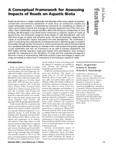
Location of study area in northeast Kansas.
National Land Cover Dataset Classification System (Vogelmann et al., 2001).
Water Open water Perennial ice/snow Developed Low intensity residential High intensity residential Commercial/industrial Barren Bare rock/sand/clay Quarries/strip mines Transitional Forested Deciduous forest Evergreen forest Mixed forest Shrubland Shrubland Non-natural woody Orchards/vineyards Herbaceous natural Grasslands/herbaceous
Western Corn Belt Ecoregion Nemaha NRD imizing cost-share program resources. Geographic information system (GIS)-guided assessments completed for stakeholders’ issues of concern can determine general areas where multiple goals can be achieved. Research suggests that one of the most effective approaches for riparian restoration in regards to terrestrial wildlife is to protect the remaining habitat patches and to restore structural connectivity in the gaps between these remnant riparian areas (Yount and Niemi, 1990; Freeman et al., 2003). Reestablishing riparian vegetation in these gaps provides critical habitat, restores linkages between patches, and promotes dispersal and gene flow between wildlife populations— crucial factors for maintaining long-term species survival (Noss and Harris, 1986; Frissell, 1997). Using this strategy, the habitat requirements for a suite of wildlife species that predominately use riparian areas can help identify riparian remnants and be used to develop a basic indicator of connectivity. The premise for this connectivity is that
210
JOURNAL OF SOIL AND WATER CONSERVATION S| O 2004
riparian remnants must be close enough to other riparian patches to facilitate exchange of individuals. This strategy has been used in upland corridors but has not been applied in riparian areas (Brooker et al., 1999). Based upon this approach, the goal of this study was to develop a GIS-based method using readily available data for locating where riparian buffers could be implemented to benefit terrestrial wildlife that primarily use riparian areas for habitat and movement corridors in northeast Kansas. The specific objectives of the study were to: (1) identify riparian remnants; (2) determine where buffers could be implemented to reestablish connectivity between remnants; and (3) identify road barriers to riparian connectivity. Our intent is for this method to serve as a potential template for use at larger scales such as the western Corn Belt ecoregion. Methods and Materials The study was conducted in the Soldier Creek watershed in northeast Kansas, a 500
Herbaceous planted/cultivated Pasture/hay Row crops Small grains Fallow Urban/recreational grasses Wetlands Woody wetlands Emergent herbaceous wetlands
km2 (193 mi2 ) region located within the western Corn Belt ecoregion (Figure 1). Once covered with tallgrass prairie, over 90 percent of the western Corn Belt ecoregion is now used extensively for cropland and pasture. A combination of nearly level to gently rolling glaciated till plains and hilly loess plains, an average annual precipitation of 63 to 89 cm (25 to 35 in), which occurs mainly in the growing season, and fertile, warm soils make this one of the most productive areas for corn and soybean in the world (Omernik, 1987). Prior to agricultural development, riparian vegetation in the ecoregion was a mosaic of vegetation types, including woodland, wetlands, and savannah communities (Robertson et al., 1997). An 1878 agricultural census for Cloud County, Kansas recorded forested riparian
Figure 3 areas varying in width from 50 to 400 m (164 to 1312 ft) consisting of cottonwood (Populus spp.), ash (Fraxinus spp.), hackberry (Celtis spp.), and oak (Quercus spp.) (KSBA, 1878). Today riparian areas in this ecoregion are highly disturbed, but since some of these areas were difficult to convert to crop production, they are also one of the few habitat types remaining partially intact (Stauffer and Best, 1980). The resulting riparian landscape pattern consists of riparian remnants separated by areas that are cropped to the edge or nearedge of the stream channel. We reviewed existing habitat and dispersal data for several wildlife species in the ecoregion that may serve as indicators of riparian connectivity: the meadow jumping mouse (Zapus hudsonius), tiger salamander (Ambystoma tigrinum), southern flying squirrel (Glaucomys volans), and eastern tiger swallowtail butterfly (Papilio glaucus). These species were selected because they (1) are primarily found in the riparian communities in the ecoregion; (2) generally do not utilize cropland habitats; (3) have relatively low dispersal capabilities, providing a conservative estimate of connectivity; and (4) are documented to use riparian corridors for dispersal (Quimby, 1951; Baker, 1983; Semlitsch, 1983; Choate et al., 1991; NatureServe, 2003). Grassland wildlife species that had limited historic use of riparian areas were not considered in the analysis since there is less than 5 percent of native grassland habitat intact in the western Corn Belt ecoregion (Ricketts et al., 1999). Conservation of these grassland-obligate species will not be significantly impacted by restoration of riparian areas instead will require restoration of large areas of grassland (Herkert, 1994). Developing connectivity thresholds for species is a challenging task due to the many factors that can influence dispersal including patch size and quality along with seasonal factors. Reducing complex interactions to basic rules is overly simplistic but the alternative of not incorporating knowledge into the planning process because it is incomplete is unproductive. To minimize the problems associated with this approach, local wildlife experts were consulted on these riparianobligate species. We selected a generic minimum riparian patch size of 0.1 ha (0.25 ac) and a dispersal distance threshold of 0.16 km (525 ft). These parameters do not represent a specific species but rather a conservative minimum based on the species reviewed. If
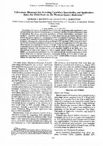
A diagram of the riparian connectivity zone and a critical gap that exceeds the 0.16 km distance threshold between riparian vegetation remnants.
Clipped riparian zone (Width varies with stream order)
Riparian vegetation remnant (≥ 0.1 ha)
Dispersal distance (≤ 0.16 km)
Connectivity zone
Critical gap (Width varies)
connectivity is achieved for these standards, it is assumed that connectivity will be achieved for many species with similar or greater dispersal capabilities. While this approach will not capture the complexity of species dispersal, it should provide a coarse-filter method for determining where to restore gaps in riparian areas. The primary dataset in the GIS-guided assessment was the United States Geologic Survey (USGS) National Land Cover Dataset, a 21-land cover classification scheme interpreted from Landsat Thematic Mapper satellite data taken during the early 1990s (Vogelmann et al., 2001) (Figure 2). In addition to satellite data, scientists developing this dataset used a variety of supporting information including topography, census, agricultural statistics, soil characteristics, other land cover maps, and wetland data to determine and label land cover types. This 30-meter
(98 ft) spatial resolution dataset, created for large area applications such as watershed management and environmental inventories, was used in this study to determine riparian vegetation remnants along streams. The stream network, a 1:100,000-scale vector dataset, was acquired from the U.S. Census Bureau’s Topologically Integrated Geographic Encoding Referencing (TIGER) database. Land cover data were clipped out along the streams in the Soldier Creek watershed using fixed-width buffer distances based on Horton-Strahler stream orders: first-order = 80 m (262 ft), second-order = 100 m (328 ft), and third-order = 120 m (394 ft) (Horton, 1945; Strahler, 1957). For instance, land cover data were extracted for 40 m (131 ft) along both sides of first-order streams for a total width of 80 m (262 ft). Higher order streams had a wider distance since they typically have a more extensive floodplain and larger spatial
S| O 2004
VOLUME 59 NUMBER 5
211
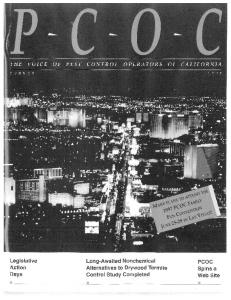
Figure 4 Riparian connectivity assessment for the Soldier Creek watershed, Kansas.
Riparian vegetation and connectvity zone Critical gap Potential road barriers
4
0
4
8
kilometers
extent of riparian vegetation (Vannote et al., 1980). These widths were selected since they generally captured the riparian remnants in their entirety. This subset of land cover data allowed for an easy, approximate delineation of the riparian area for the connectivity analysis. Within this subset of data, we reclassified the forested, shrub land, and wetland vegetation communities into a single group called “riparian vegetation.” Ideally, native grassland should be included in this reclassified “riparian vegetation” since this plant community was a historical component in the lower stream orders (Robertson et al., 1997). However, grassland cover was not included in this regrouped classification because this cover type was predominantly hayfields or
212
JOURNAL OF SOIL AND WATER CONSERVATION S| O 2004
non-native pasturelands misclassified as native grasslands (USGS, 2003). Although this is a shortcoming in the National Land Cover Dataset, it is diminished by the fact that there is less than 5 percent of native grassland remaining in the region (Ricketts et al., 1999). Hayfields and non-native pastures provide little habitat value in comparison to native grasslands due to patch size and vegetation structure and composition (Herkert 1994). Each individual patch of riparian vegetation 0.1 ha (0.25 ac) or greater in area was buffered by 1⁄2 the dispersal threshold distance of 0.08 km (262 ft). Where the dispersal distances touch or overlap, the gap between the remnants is theoretically close enough for successful movement between the riparian
remnants for species with low dispersal capabilities and is delineated as a connectivity zone (Figure 3). Areas that exceed the connectivity threshold are delineated as “critical gaps” that could benefit from being reconnected using riparian buffers. Barriers to riparian connectivity are defined as any element that significantly restricts flows of energy, materials, or species (Forman, 1995). Roads are one of the primary barriers for species moving from one habitat to another, particularly for small mammals and amphibians with low dispersal capabilities, such as the meadow jumping mouse or tiger salamander (Ashley and Robinson, 1996; Trombulak and Frissell, 2000). Using road data from the Kansas Department of Transportation, this assessment identifies where major roads intersect riparian corridors, allowing resource managers to consider the potential impacts of these barriers on riparian buffer locations. For instance, increasing riparian connectivity near a road crossing may promote road mortality if a safe passage is not provided under or over the road. In some cases, these barriers can be retrofitted to minimize hazards for various wildlife species by providing travel culverts under the road (FHWA, 2003). Results and Discussion Figure 4 illustrates the result of the riparian connectivity assessment for the Soldier Creek watershed. The assessment located riparian remnants that were greater than or equal to 0.1 ha (0.25 ac) in size and critical gaps that exceeded the dispersal distance threshold of 0.16 km (525 ft). The critical gaps, shown in black, denote where riparian buffers could be implemented to reestablish connectivity, while the grey color represents existing riparian vegetation and the connectivity zone. In this study, 126 km (78 mi) or 22 percent of the total length of streams analyzed in the watershed were classified as critical gaps (Table 1). First-order streams showed the greatest overall length with critical gaps of 113 km (70 mi) compared to second-order streams with 11 km (7 mi) and third-order streams with 2 km (1 mi). This difference may be attributed to the biophysical factors that allow first-order riparian vegetation to be vulnerable to removal. First-order streams in the region may be intermittent, may flood less frequently due to smaller contributing areas, and are less incised, allowing landowners to easily remove riparian vegetation and
Table 1. Results of the riparian connectivity assessment for the Soldier Creek watershed. Total stream length (km)
Stream length in critical gap (km)
Stream length in critical gap (%)
First-order Second-order Third-order Total
378 101 95 574
113 11 2 126
30 11 2 22
assessment was evaluated using digital orthophotos from USGS, which were taken during the same time period (early 1990s) as the satellite images used to develop the National Land Cover Dataset. The 1-m (3-ft) resolution orthophotos are at a much finer scale than the 30-m (98-ft) resolution National Land Cover Dataset, which the riparian connectivity assessment was based upon. Due to this difference in resolution, the riparian connectivity method is expected to have errors in relation to the coarseness of data in the National Land Cover Dataset. Accuracy of the assessment was evaluated by comparing the critical gaps identified in the connectivity assessment with the orthophotos
to determine if there were actual gaps in riparian vegetation. Approximately 81 percent of the critical gaps identified in the connectivity assessment were actual gaps; the other 19 percent of the gaps had an adequate, existing riparian buffer based on the orthophotos (Table 3). Accuracy was relatively consistent between stream orders. The error that did occur was primarily the result of the 30-m (98 ft) land cover data misidentifying existing riparian vegetation as another cover type, such as cropland or pastureland. Another type of error that could occur is the potential for critical gaps to exist that were not identified or captured by the connectivity assessment. This did not seem to be a
Table 2. Average and median stream length classified as critical gap in the Soldier Creek watershed. Stream order
Average length in critical gap (km)
Median length in critical gap (km)
First-order Second-order Third-order
0.27 0.19 0.10
0.14 0.07 0.05
Figure 5 Frequency of critical gaps in the Soldier Creek watershed for selected distance intervals.
180 160 140 120
Frequency
convert the riparian area to cropland (Vannote et al., 1980). Within first-order streams, there also appears to be patterns in the spatial distribution of critical gaps such as the concentration of gaps in the streams located in the middle section of the watershed. While this may be due to a biophysical factor, it may be more likely a result of land ownership and the potential lack of stewardship for riparian buffers by landowners, an important factor for planners to consider when promoting buffer programs in this area. Table 2 provides the average and median stream lengths classified as critical gap (average and median lengths are gap distances that exceed the 0.16 km connectivity zone—See Figure 3). The average and median critical gap lengths are considerably longer in firstorder streams compared to the higher order streams, which may be attributed to the ease of riparian vegetation removal compared to second and third-order streams. The median lengths are considerably less than the average lengths suggesting a skewed distribution. The frequency of critical gaps for selected distance intervals illustrates a concentration of gaps less than 0.1 km (328 ft) in length (Figure 5). This indicates that many gaps can be addressed with relatively short riparian buffer plantings. Figure 5 also reveals that there are a number of gaps along first-order streams that exceed 0.5 km (1640 ft). These long gap lengths suggests that many of these critical gaps may cross more than one property, highlighting the potential challenge of getting multiple landowners to cooperate on implementing a continuous riparian buffer. Figure 4 also shows where existing roads intersected riparian corridors in the Soldier Creek watershed. Although roads were not directly used in calculating critical gaps, their influence on habitat connectivity can be significant depending on road orientation and location. Some roads intersected the riparian corridor at angles close to perpendicular, minimizing the area of disturbance while other roads were more aligned with the corridor, creating a potentially more significant barrier to wildlife dispersal. Other areas of concern also include where two roads intersect in a riparian corridor as seen in the enlarged area (Figure 4). Further field reconnaissance could reveal if these areas are barriers to species movement and if there are opportunities to retrofit safe passageways through culverts or bridges. The accuracy of the riparian connectivity
Stream order
100 80 60 40 20 0 0-0.1
0.11-0.2 0.21-0.3
0.31-0.4
0.41-0.5
0.51-2.5
Critical gap length in km First-order frequency
Second-order frequency
S| O 2004
Third-order frequency
VOLUME 59 NUMBER 5
213
Table 3. Evaluation of the riparian connectivity assessment for the Soldier Creek watershed compared to digital orthophotos of the same area.
Stream order
Number of critical gaps
Number of critical gaps correctly identified a
Critical gaps correctly identified (%)
First-order 422 341 81 Second-order 59 46 78 Third-order 25 21 84 Total 506 408 81 a Based on comparing the critical gaps identified in the connectivity assessment with digital orthophotos.
problem because existing non-riparian cover types were rarely misclassified as being a riparian cover type. In general, the assessment procedure appears to slightly overestimate the number of actual critical gaps in the watershed. Limitations. There are several limitations that potential users need to consider before using this connectivity tool. Because all ecological analyses are driven by the scale of the data used, these results are strongly influenced by the 30-m (98 ft) resolution of the National Land Cover Dataset. Riparian areas in the region are relatively narrow elements in the landscape along low-order streams. One reason for using the 0.1 ha (0.25 ac) patch size (approximately the size of one cell in the National Land Cover Dataset) was to identify small riparian remnants. The error rates generated from the exercise show that it still is a challenge to correctly identify these remnants and critical gaps. Habitat connectivity along first-order streams, in particular, may not be appropriate to analyze using this method. Historic riparian vegetation along first-order streams was probably dominated by savannah or grassland rather than shrub and forest cover. However grassland was not able to be included in the assessment due to the misidentification of hayfields and pasturelands as native grassland in the National Land Cover Dataset. One suggestion is not to use to the National Land Cover Dataset for analyzing first-order streams. Planning for riparian management along first-order streams will require higher quality land cover data, possibly developed from the digital orthophotos. The method does not take into consideration that different land uses offer varying degrees of resistance for species movement between the riparian remnants (Sutcliffe et al., 2003). For instance, urban land use occurring in the riparian area may be more of a barrier than row cropland for species movement. Since the majority of the land use occurring in the critical gaps for the study area reported was in row crop or pastureland, there was not enough variability to warrant
214
JOURNAL OF SOIL AND WATER CONSERVATION S| O 2004
weighting the land uses differently;however,this may be necessary in areas where more developed land uses intrude into the riparian area. Riparian habitat quality will strongly influence long-term viability and dispersal success for most species. Currently there is no way to reliably address habitat quality of the existing riparian remnants with available data. For instance, some riparian remnants in the study area may have little habitat value due to overgrazing by livestock. This illustrates the need for resource managers to use site visits with landowners to make buffer planning and design decisions. Potential applications. With these limitations in mind, this method is probably best suited for large-area planning such as single or multi-county resource inventories or for USGS 8-digit hydrologic unit watershed assessments used to help focus riparian buffer implementation efforts. The assessment procedure does not indicate which gaps are more important to address than others, but it may be possible to apply some simple guidelines to rank areas. Although lower-order streams in this watershed have the greatest stream length in critical gaps, it may be more effective to concentrate on implementing riparian buffers on higher-order streams, yielding more benefits for wildlife due to the increase in overall habitat area associated with higher-order streams (Nilsson et al., 1989; Spackman and Hughes, 1995). Implementing buffers in short critical gaps may be more efficient due to the increased likelihood that the gap occurs entirely on one property, facilitating project coordination. In the case where a critical gap covers several properties, the assessment may be a valuable tool to visually illustrate to multiple landowners how they are important links in creating a more connected riparian system. It may also be more beneficial to initially focus on restoring critical gaps that are away from roads, providing longer, more continuous riparian corridors that are not impacted by roads (Forman, 1995). The assessment may also serve as a valuable
benchmark for monitoring trends in riparian connectivity if the same methodology is applied to future land cover data, such as the new National Land Cover Dataset currently being developed from satellite images from the early 2000s. In addition to simple summaries of kilometers or hectares of conservation practices applied, decision- and policymakers now want indicators that provide a measure of the ecological functions achieved with conservation practices on agricultural lands (Piorr, 2003). There are many efforts currently underway to develop effective but realistic-to-apply indicators of environmental sustainability in agricultural landscapes (Riley, 2001; Buchs, 2003; Piorr, 2003). The riparian connectivity assessment based on a suite of local species can serve as one function-based approach in the set of potential indicators. The method describe in this paper should be viewed as a general template, which can be modified based on available data, selected species, and local expert input. Summary and Conclusion Although there are assessment methods being developed to prioritize riparian areas for the protection of biodiversity in agricultural landscapes (e.g., Iverson et al., 2001), very few take the next step and offer guidance on where riparian areas should be restored for wildlife. Our method attempts to identify locations where buffers could be implemented to reestablish natural connectivity of riparian areas. Requiring minimal data sets and GIS skills, this assessment method should be feasible for use by resource planners, improving buffer planning efforts where one of the objectives is promoting riparian habitat connectivity. The most significant benefit of using GISguided assessments in conservation planning is the opportunity to combine different assessments to determine locations where multiple objectives can be accomplished with riparian buffers. We have developed several suitability assessments for determining optimal locations for growing specialty products in riparian buffers that can be sustainably harvested for commercial use including medicinals and products for the decorative floral industry (Bentrup and Leininger, 2002). In addition, methodologies are currently being developed to select areas for riparian buffers to filter agricultural pollutants from surface runoff and shallow groundwater flow. The utility of these assessments depends on
each analysis method to be kept relatively simple and based on available data in order to promote the use and combination of assessment results. By combining these and other resource assessments, areas can be identified where environmental protection and agricultural production goals can be attained at the same time with a buffer investment, enhancing the acceptance and long-term adoption of these practices. Acknowledgements Funding for this effort was provided through the U.S. Department of Agriculture National Agroforestry Center, which is part of the Rocky Mountain Research Station, and the University of Missouri Center for Agroforestry under cooperative agreements 58-6227-1-004 with the Agricultural Research Service (ARS) and CR 826704-01-2 with the U.S. Environmental Protection Agency (EPA). The results presented are the sole responsibility of the principal investigator and may not represent the policies or positions of the ARS or EPA. The authors would like to thank Michele Schoeneberger, Gary Wells, Lane Eskew, Tim Leininger, and three anonymous reviewers for their helpful feedback on this project.
References Cited Ashley, E.P. and J.T. Robinson. 1996. Road mortality of amphibians, reptiles, and other wildlife on the Long Point Causeway, Lake Erie, Ontario. Canadian Field Naturalist 110:403-412. Baker, R.H. 1983. Michigan Mammals. Michigan State University Press, Detroit, Michigan. Bentrup, G. and T. Leininger. 2002. Agroforestry: mapping the way with GIS. Journal of Soil and Water Conservation (57):148a-153a. Brooker, L., M. Brooker, and P. Cale. 1999. Animal dispersal in fragmented habitat: measuring habitat connectivity, corridor use, and dispersal mortality. Conservation Ecology [online] 3(1).Available from the Internet URL: h t t p : / / w w w. c o n s e c o l . o r g / v o l 3 / i s s 1 / a r t 4 Verified: 11/23/2003. Buchs, W. 2003. Biotic indicators for biodiversity and sustainable agriculture-introduction and background. Agriculture, Ecosystems, and Environment 98:1-16. Burbrink, F.T., C.A. Phillips, and E.J. Heske. 1998. A riparian zone in southern Illinois as a potential dispersal corridor for reptiles and amphibians. Biological Conservation 86:107-115. Choate, J.R., D.W. Moore, and J.K. Frey. 1991. Dispersal of the meadow jumping mouse in Northern Kansas. Prairie Naturalist 23:127-130. Federal Highway Administration (FHWA). 2003. Critter crossings: Linking habitats and reducing roadkill. Department of Transportation, Federal Highway Administration. [online] URL: http://www.fhwa.dot. gov/environment/wildlifecrossings/index.htm Verified: 11/23/2003. Forman, R.T. 1995. Land mosaics: The ecology of landscapes and regions. Cambridge University Press, Cambridge, Maryland.
Freeman, R.E., E.H. Stanley, and M.G.Turner. 2003.Analysis and conservation implications of landscape change in the Wisconsin River floodplain, USA. Ecological Applications 13:416-431. Frissell, C.A. 1997. Ecological principles. Pp. 96-115. In: J. Williams, C.A. Wood, and M.P. Dombeck (eds). Watershed Restoration: Principles and Practices. American Fisheries Society, Bethesda, Maryland. Hanson, J.S., G.P. Malanson, and M.P. Armstrong. 1990. Landscape fragmentation and dispersal in a model of riparian forest dynamics. Ecological Modeling 49:277-296. Herkert, J.R. 1994. The effects of habitat fragmentation on Midwestern grassland bird communities. Ecological Applications 43:461-471. Hilty, J.A. and A.M. Merenlender. 2004. Use of riparian corridors and vineyards by mammalian predators in northern California. Conservation Biology 18:126-135. Horton, R.E. 1945. Erosional development of streams and their drainage basins: Hydrophysical approach to quantitative morphology. Geological Society of America Bulletin 56:275-370. Iverson, L.R., D.L. Szafoni, S.E. Baum, and E.A. Cook. 2001. A riparian wildlife habitat evaluation scheme developed using GIS. Environmental Management 28:639-654. Kansas State Board of Agriculture. 1878. First Biennial Report of the State Board of Agriculture to the Legislature of the State of Kansas, for the Years 1877-8. Topeka, Kansas: Kansas State Board of Agriculture. Rand, McNally & Co., Printers and Engravers, Chicago, Illinois. Machtans, C.S., M.A.Villard, and S.J. Hannon. 1996. Use of riparian buffer strips as movement corridors by forest birds. Conservation Biology 10:1366-1379. Maisonneuve, C. and S. Rioux. 2001. Importance of riparian habitats for small mammal and herptofaunal communities in agricultural landscapes of southern Québec. Agriculture, Ecosystems, and Environment 83:165-175. Naiman, R.J., H. Decamps, and M. Pollock. 1993. The role of riparian corridors in maintaining regional biodiversity. Ecological Applications 3:209-212. National Research Council (NRC). 2002. Riparian areas: Functions and strategies for management. National Academy Press,Washington, D.C. NatureServe. 2003. An Online Encyclopedia of Life. 2000. Version 1.1. Association for Biodiversity Information, Arlington,Virginia. [online] URL: http://www.natureserve.org.Verified: 10/17/2003. Nilsson, C., G. Grelsson, M. Johansson, and U. Sperens. 1989. Pattern of plant species richness along riverbanks. Ecology 70:77-84. Noss, R.F. and L.D. Harris. 1986. Nodes, networks, and MUMs: Preserving diversity at all scales. Environmental Management 10:299-309. Omernik, J.M. 1987. Ecoregions of the conterminous United States. Map (scale 1:7,500,000). Annals of the Association of American Geographers 77:118-125. Piorr, H.R. 2003. Environmental policy, agri-environmental indicators, and landscape indicators. Agriculture, Ecosystems and Environment 98:17-33. Quimby, D.C. 1951. Life history and ecology of the jumping mouse, Zapus hudsonicus. Ecological Monographs 21:61-95. Ricketts,T.H., Dinerstein, E., Olson, D.M., Loucks, C.J., and Eichbaum, W. 1999. Terrestrial Ecoregions of North America: A Conservation Assessment. Island Press, Washington, D.C. Riley, J. 2001. The indicator explosion: local needs and international challenges. Agriculture, Ecosystems and Environment 87:119-120.
Robertson, K.R., R.C. Anderson, and M.W. Schwartz. 1997. The tallgrass prairie mosaic. Pp. 55-87. In: M.W. Schwartz (ed) Conservation In Highly Fragmented Landscapes. Chapman and Hall, New York, New York. Semlitsch, R.D. 1983. Terrestrial movements of an Eastern Tiger Salamander. Herpetological Review 14:112-113. Spackman, S.C. and J.W. Hughes. 1995. Assessment of minimum stream corridor width for biological conservation: species richness and distribution along mid-order streams in Vermont, USA. Biological Conservation 71:325-332. Stauffer, D.F. and L.B. Best. 1980. Habitat selection by birds of riparian communities: evaluating effects of habitat alterations. Journal of Wildlife Management 44:1-15. Strahler, A.N. 1957. Quantitative analysis of watershed geomorphology. American Geophysical Union Transactions 38:913-920. Sutcliffe, O.L., V. Bukkestuen, G. Fry, and O.E. Stabbetorp. 2003. Modeling the benefits of farmland restoration: methodology and application to butterfly movement. Landscape and Urban Planning 63:15-31. Thomas, J.W., C. Maser, and J.E. Rodiek. 1979. Wildlife Habitats in Managed Forests. U.S. Department of Agriculture Forest Service Handbook No. 553. Tockner, K. and J.A. Stanford. 2002. Riverine floodplains: Present state and future trends. Environmental Conservation 29:308-330. Trombulak, S.C. and C.A. Frissell. 2000. Review of ecological effects of roads on terrestrial and aquatic communities. Conservation Biology 14:18-30. U.S. Geologic Survey (USGS). 2003. Accuracy Assessment of 1992 National Land Cover Dataset. [online] URL: http://landcover.usgs.gov/accuracy/index.asp#results Verified: 03/02/04. Vannote, R.L., G.W. Minshall, K.W. Cummins, J.R. Sedell, and C.E. Cushing. 1980.The river continuum concept. Canadian Journal of Fisheries and Aquatic Sciences 37:130-137. Vogelmann, J.E., S.M. Howard, L. Yang, C.R. Larson, B.K. Wylie, and N.Van Driel. 2001. Completion of the 1990s National Land Cover Data Set for the conterminous United States from Landsat thematic mapper data and ancillary data sources. Photogrammetric Engineering and Remote Sensing 67:650-652. Yount, J.D. and G.J. Niemi. 1990. Recovery of lotic communities from disturbance—a narrative review of case studies. Environmental Management 14:547-569.
S| O 2004
VOLUME 59 NUMBER 5
215