Galactic Swarm Optimization using Artificial Bee

2017 Fifteenth International Conference on ICT and Knowledge Engineering

Galactic Swarm Optimization using Artificial Bee Colony Algorithm Ersin Kaya

İsmail Babaoğlu

Department of Computer Engineering Selçuk University, Faculty of Engineering Konya, Turkey [email protected]

Department of Computer Engineering Selçuk University, Faculty of Engineering Konya, Turkey [email protected]

Halife Kodaz Department of Computer Engineering Selçuk University, Faculty of Engineering Konya, Turkey [email protected]

Abstract—Galactic swarm optimization (GSO) algorithm is a novel meta-heuristic algorithm inspired by the motion of stars, galaxies and superclusters of galaxies under the influence of gravity. The GSO algorithm utilizes multiple cycles of exploration and exploitation in two levels. The first level covers the exploration, and different subpopulations of the candidate solutions are used for exploring the search space. The second level covers the exploitation, and best solutions obtained from the subpopulations are considered as a superswarm and used for exploiting the search space. The first implementation of GSO algorithm was presented by using particle swarm optimization algorithm (PSO) algorithm on both first and second levels. This study presents the preliminary results of an implementation of GSO algorithm by using artificial bee colony (ABC) algorithm on the first level and PSO algorithm on the second level. Due to the better exploration characteristics of ABC algorithm over PSO algorithm, this suggestion covers the usage of ABC algorithm on the first level, and the usage of PSO algorithm on the second level. The proposed approach is tested on 20 well-known online available benchmark problems and preliminary results are presented. According to the experimental results, the proposed approach achieves more successful results than the basic GSO approach. Keywords—galactic swarm optimization; artificial bee colony algorithm, particle swarm optimization algorithm, meta-heuristic

I. INTRODUCTION Many evolutionary algorithms were proposed for solving continuous optimization problems. According to their inspiration and convergence mechanisms, these algorithms have some advantages over each other in terms of exploration and exploitation characteristics. Particle swarm optimization (PSO) algorithm was developed inspiring the schooling behavior of the fishes or flocking behavior of birds [1], cuckoo search algorithm was developed by inspiring the obligate brood parasitism of some species of cuckoo [2], ant colony optimization algorithm was developed by inspiring the

978-1-5386-2117-2/17/$31.00 ©2017 IEEE

behavior of the ants during the foraging between nest and the food source [3], artificial bee colony (ABC) algorithm was developed by inspiring the foraging and dancing behavior of the honey bees [4], firefly algorithm was developed by inspiring the flashing behavior of the fireflies [5], fruit fly algorithm was developed by inspiring the foraging behavior of the fruit flies [6] and bat algorithm was developed by inspiring the echolocation behavior of the microbats [7]. There are also many different meta-heuristic algorithms developed by inspiring behaviors from the nature which can be found in the literature. Among the various meta-heuristic algorithms, PSO is one of the most researched and developed algorithm. There are many improved versions of PSO in literature including standard PSO namely SPSO2011 [8], modified quantum-based PSO [9], modified bare-bones PSO [10], chaotic catfish PSO [11] and adaptive PSO [12]. Also, many improved versions of ABC can be obtained from the literature including modified ABC [13, 14], ABC algorithm with memory [15], directed ABC algorithm [16], memetic search in ABC algorithm [17] and crossover-based ABC [18]. In order to achieve better results, researchers try to improve the success rate of the algorithms by hybridization or some enhancements over the structure of the algorithms. Besides, there also many multi-swarm optimization algorithms developed for achieving better models for continuous optimization problems [19-23]. Galactic swarm optimization (GSO) algorithm is a recently developed meta-heuristic algorithm inspired by the motion of stars, galaxies and superclusters of galaxies under the influence of gravity[24]. The GSO algorithm utilizes multiple cycles of exploration and exploitation in two levels. The first level covers the exploration, and different subpopulations of the candidate solutions are used for exploring the search space. The second level covers the exploitation, and best solutions obtained from the subpopulations are considered as a superswarm and used for exploiting the search space.

The first implementation of GSO algorithm was presented by using PSO algorithm on both first and second levels. This study presents the preliminary results of an implementation of GSO algorithm by using ABC algorithm on the first level and PSO algorithm on the second level. Due to the better exploration characteristics of ABC algorithm over PSO algorithm, this suggestion covers the usage of ABC algorithm on the firstlevel, and the usage of PSO algorithm on the secondlevel. The rest of the paper is organized as follows; introduction of ABC, PSO, GSO algorithms and proposed approach, and demonstration of the benchmark functions are presented in Section 2, experimental results are presented in Section 3, and the study is finalized by discussing in Section 4.

this food source become a scout bee and start searching another food source randomly. If the scout bee finds a proper food source, then it becomes an employed bee. According to the algorithm, the number of employed bees are equal to the onlooker bees. TABLE I. a

b

BENCHMARK FUNCTIONS USED IN EXPERIMENTS c

No

N -S - C

F1

Sphere [-100,100] – US

F2

Elliptic [-100,100] –UN

F3

Function 1

(⃗) =

2 =1

2

( ⃗) =

6 ( −1)/( −1) 2

(10 ) =1

SumSquares [-10,10] –US

3

( ⃗) =

2 =1

II. MATERIALS AND METHODS A. Benchmark Functions used in Experiments In order to evaluate the compared methods, 20 well-known benchmark functions are used in this study. Depending on their characteristics, the benchmark functions can be classified concerning modality and separability. According to the modality, the functions can be an either unimodal or multimodal function, and according to the separability, the functions can be an either separable or non-separable function. Unimodal functions are described as having single local optimum, and also this optimum is the global optimum. Multimodal functions have more than one local optimum and one or more global optimum. On the other hand, while separable functions can be written as sum of the n functions, non-separable functions cannot be parsed just like the separable functions due to the interrelation between the variables [25]. The benchmark functions and their properties are given in Table 1. The classification of the functions are given in class column on the table, and US, UN, MS and MN stands for unimodal-separable, unimodal-nonseparable, multimodalseparable and multimodal-nonseparable respectively. B. Artificial Bee Colony Algorithm Artificial bee colony algorithm was suggested by Karaboga [4] for solving numerical optimization problems. ABC algorithm was suggested by inspiring foraging and dancing behavior of honey bees. There are two types of honey bees. The first type of the honey bees are called employed bees which are responsible for collecting nectar from the food sources which are accepted as possible solutions in the algorithm. The second type of honey bees are called unemployed bees, and it is separated into two sub-types namely onlooker bees and scout bees. The onlooker bees search other food source positions around the hive considering the information shared by the employed bees. The employed bees use waggle dance to share information with the other bees in the hive. Scout bees are another sub-type of unemployed bees, and they are responsible for searching the environment without any information obtained from the other bees in order to get new food sources. According to the algorithm, there can only be one scout bee in the population after some iteration cycles and assumption. If a food source is not improved within a certain amount of time, which is known as limit, with either employed or onlooker bees, the employed bee investigating

F4 F5 F6 F7 F8 F9 F10 F11

F12

SumPower [-10,10] –MS Schwefel2.22 [-10,10] –UN Schwefel2.21 [-100,100] –UN Step [-100,100] –US Quartic [-1.28,1.28] –US QuarticWN [-1.28,1.28] –US Rosenbrock [-10,10] –UN Rastrigin [-5.12,5.12] –MS

4

Griewank [-600,600] –MN Schwefel2.26 F14 [-500,500] –UN

⃗ =

| |+

⃗ =

{| |, 1 ≤ ≤ }

⃗ =

| |

(⌊

+ 0.5⌋)

⃗ = ⃗ =

[0,1)

+

⃗ =

[100(

−

− 1) ]

) +(

⃗ =

[

− 10 cos(2

) + 10]

⃗ =

[

− 10 cos(2

) + 10]

| |< =

⃗ =

(2 )

| |≥

2

1 4000

−

⃗ = 418.98 ∗ ⃗ = −20

F15

| |( +1) =1

Non-Continuous Rastrigin [-5.12,5.12] –MS

F13

( ⃗) =

cos

−

2 1 2 √

+1

| |

sin 1

−0.2

Ackley [-32,32] –MN

1

1

−

cos(2

)

+ 20 + ⃗ =

(

10

) + + 10 +(

F16

Penalized1 [-50,50] –MN

(

− 1) [1

(

)]

− 1)

+ 1 = 1+ (

(

4 − ) 0

= (

− )

( , 10,100,4)

+ 1)

, , ,

> − ≤

≤

< −

⃗ =

1 10

(

+ F17

Penalized2 [-50,50] –MN

Alpine [-10,10] –MS

F19

Levy [-10,10] –MN

⃗ = ⃗ =

(

(3 )] − 1) [1

+

(2

| (

+ +| ⃗ =

F20

( , 5,100,4)

∙ sin( ) + 0.1 ∙ (3

(

cos 2

[

− = 0.5,

= 3,

| )]

(3 ) − 1|[1 +

(3

0.5)]

= 20 a. b.

Search Range Class

The ABC algorithm has four basic phases. These phases can be called as initialization phase, employed bee phase, onlooker bee phase and scout bee phase, and also these phases are explained briefly as follows; Initialization Phase: In the initial phase of the ABC algorithm, solutions are generated randomly for employed bees by using (1). ,

=

+

−

(1) th

where = 1, … , , = 1, … , , , is the j dimension of the ith employed bee and are upper and lower boundaries of the dimension respectively, is a random number within therange [0,1], is the number of employed bees and is the dimensionality of the problem. Employed Bee Phase: New candidate solutions are generated in this phase. First of all, the solution of an employed bee is copied as the candidate solution ( = ) and one dimension of this solution is updated using (2). ,

=

,

+

,

−

,

=

Name

c.

|

ℎ

( 3)

Onlooker Bee Phase: In this phase, each onlooker bee selects an employed be in order to improve the solution quality of the selected employed bee. Selection of the employed bee is accomplished by using the roulette wheel selection technique over the fitness values of the employed bees, and calculated as in (4).

)]

+ 0.5)

cos(2

≥0

where is the fitness value of the ith employed bee, is the objective function value of the ith employed bee. According to the calculated fitness values, the employed bee is replaced with the candidate solution if the fitness value of the candidate solution is better than the fitness value of the employed bee ( = ). In case of a replacement of the employed bee with the candidate solution, the abandonment counter is reset to 0, otherwise this counter is increased by 1.

)]

− 1) [1 +

Weierstrass [-0.5,0.5] –MN

− 1) [1

+ +(

+ F18

1 = 1+ 1+|

)

( 2)

where , is the jth dimension of the ith candidate solution, , ∈ {1, … , }, ∈ {1, … , } and ≠ , is the jth , th th dimension of the i employed bee, , is the j dimension of the kth employed bee and is a random number within [-1,1]. In this phase, the neighbor ( ) of the employed bee and also the dimension which is going to be updated ( ) are selected randomly. After the candidate solutions were produced, and the objective value of the solution concerning the optimization problem were calculated, the fitness value of the candidate solutions and employed bees are obtained using (3).

( ∑

4)

where, is the probability of the ith employed bee whether is selected or not. After the selection of the employed bee by using the roulette wheel selection technique, the onlooker bee tries to improve the quality of the solution, and this is done by using (2). After calculating fitness values of the new solutions found by the onlooker bee, the employed bee is replaced with the onlooker bee if the fitness value of the onlooker solution is better than the fitness value of the employed bee ( = ). In case of a replacement of the employed bee with the onlooker bee, the abandonment counter is reset to 0, otherwise this counter is increased by 1. C. Particle Swarm Optimization Algorithm PSO algorithm was firstly introduced by Kennedy and Eberhard, and developed by inspiring flocking behavior of the birds and schooling behavior of the fishes [1]. PSO algorithm is a population based optimization technique. Each potential solution in PSO is defined as a particle, the agent, and the particles try to find the optimum solution by improving the best particles solutions which are generated randomly among the solution space at the initialization step. During the iterative workflow of the algorithm, each particleis updated by not only using the best solution obtained by the particle so far but also the best solution obtained by the swarm so far. PSO is one of the most commonly used optimization algorithms due to the few configuration parameters, easily understandable and implementable structure. After randomly generation of the particles, which are also the solutions, the velocity of each particle is calculated by using (5) and each particle is updated by using the velocity as given in (6). ( + 1) =

( )+ +

( + 1) =

( ( ) − ( )) ( ( ) − ( )) ( )+

()

(5) (6)

( ) is the velocity of ithparticle at iteration t, ( ) is where the position of ithparticle at iteration t, and are uniformly distributed random number within the range [0,1], and are the acceleration constants, also called as cognitive and social parameters, which controls the search direction towards the personal best or global best solutionrespectively, ( ) is the personel best solution of ithparticle at iteration t, ( ) is the best solution found so far at iteration t.

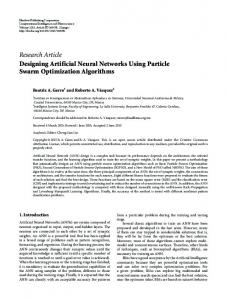
GSO algorithm which is implemented by PSO algorithm is given in Fig. 1.

The iterative workflow structure of the PSO algorithm can be summarized as follows; 1. Particles are generated randomly and initial velocities are set to 0. 2. Velocity of each particle is calculated using (5) 3. Each particle is updated as given in (6) using concerned velocity 4. Fitness value of each particle is obtained 5. Personal best values of each particle and the global best value of the swarm is updated. 6. Steps 2-6 are repeated until the stopping creation is achieved. D. Galactic Swarm Optimization Algorithm GSO algorithm is a meta-heuristic algorithm inspired by the motion of stars, galaxies and superclusters of galaxies under the influence of gravity[24]. As the stars within the galaxy affects each other, galaxies also affect each other. Agents are grouped in order to find solutions in GSO algorithm. These agents represent the stars, and agent groups represent the galaxies. GSO algorithm is a two-leveled optimization method. Each level is an optimization method that operates independently within itself with a restriction of taking initial population from outside. These optimization methods can be chosen as desired. PSO algorithm was chosen on the basis implementation of the GSO algorithm. In this implementation, best solutions related with each group is obtained by PSO in the first level. On the second level, a superior population, namely superswarm, is generated among the best solutions of the groups, and then the optimum solution is investigated using PSO algorithm [24].Multi-layered population structure of GSO algorithm can be given as in (7). ∈

: = 1,2, … ,

∈

:

=

( )

(7)

= Considering the structure which is given in (7) in the GSO algorithm, solutions are divided into subpopulations each consist solutions. denotes the jthagent within the ith sub population. Set denotes the ith sub population, and ( ( )) denotes the agent having the best solution within the population . The set is the superswarm which consist of agents having the best solutions obtained from the related subpopulations. First and second levels are repeated a defined number of times, and the maximum number of repetition is called as epoch. The pseudo code of the originalversion of

Fig. 1. Pseudo code of basis GSO algortihm [24]

E. Proposed Method In optimization methods, it’s expected that both exploration and exploitation characteristics of the algorithm be powerful in order to achieve successful results. Exploration deals with the optimum global search of the solutions within the search space. On the other hand, exploitation deals with the optimum local search over the optimum global solutions obtained by exploration within the search space. As stated in [24], GSO algorithm is not only an approach but also a framework for optimization problems. Along with the original version, many different optimization techniques could be implemented in first, second or both first and second levels. PSO algorithm was used in both first and second levels in the original version of the GSO algorithm. In general, exploration is provided in the first level, and exploitation is provided in the second level in the GSO algorithm. PSO algorithm is an easy to use optimization algorithm which has a powerful exploitation characteristic. In spite of that, ABC algorithm has more powerful exploration characteristic than PSO algorithm. For this reason, the proposed method is generated by using ABC algorithm which has a better exploration characteristic in the first level and PSO algorithm which has a better exploitation characteristic in the second level of GSO algorithm. By this implementation, it is desired to obtain a new more powerful optimization approach. In the proposed implementation of GSO algorithm, food source positions which are candidate solutions in ABC algorithm are utilized by accepting equivalent to particles which are also candidate solutions in PSO algorithm.

a.

III. RESULTS AND DISCUSSION For all experiments, the maximum number of function evaluation is used as the termination condition in the proposed approach. The results of the proposed approach GSO (ABCPSO) is compared with the results of the basis version of GSO (PSO-PSO). The benchmark functions are used for evaluation in 30, 60 and 100 dimensional forms. Both algorithms are run 30 times with different seeds and mean values are reported. Maximum epoch number , the number of subpopulation size and the number of agents in each subpopulation is taken as 5, 10 and 10 respectively for both algorithms. In order to provide more fair comparison of the algorithms, the maximum number of function evaluation sizes are used being equal to 225,000, 450,000 and 750,000 for 30, 60 and 100 dimensional benchmark problems respectively for both algorithms. Besides, cognitive and social parameters and are used being equal to each other as 2.05. The results of the proposed approach GSO (ABC-PSO) is compared with the original version of GSO (PSO-PSO), and the comparative results are given in Table 2, Table 3 and Table 4 for 30, 60 and 100 dimensional benchmark problems respectively. According to the comparative results, the proposed approach achieves better results for almost all benchmark problems evaluated for 30 dimension than the original version of the GSO (PSO-PSO) algorithm. None the less the original version of the GSO (PSO-PSO) algorithm achieves equal evaluation results with the proposed approach on Step benchmark function (F7) and better evaluation results on Rastrigin benchmark function (F11). For 60 dimensional problems, the proposed approach GSO (ABC-PSO) achieves better results also for almost all benchmark problems. The original version of GSO (PSO-PSO) algorithm achieves slightly better results than the proposed approach for Sphere (F1), Schwefel2.21 (F6), Quartic (F8) and Alpine (F18) benchmark functions. Experimental results for 30 dimensional problems Noa F1 F2 F3 F4 F5 F6 F7 F8 F9 F10 F11 F12 F13 F14 F15 F16 F17 F18 F19 F20

GSO (ABC-PSO)

GSO (PSO-PSO)

TABLE II. Noa F1 F2 F3 F4 F5 F6 F7 F8 F9 F10 F11 F12 F13 F14 F15 F16 F17 F18 F19 F20

Function Number

EXPERIMENTAL RESULTS FOR 60 DIMENSIONAL PROBLEMS GSO (ABC-PSO)

GSO (PSO-PSO)

Mean

Std. Dev.

Mean

Std. Dev.

5.47E-38 4.47E-15 4.63E-68 1.07E-126 2.17E-10 4.80E-77 0.00E+00 7.08E-203 2.79E-06 5.59E+00 3.66E-01 4.99E-01 3.47E-16 1.81E+03 7.38E-05 8.46E-12 4.77E-07 7.61E-05 5.94E-04 1.78E-03

2.99E-37 2.45E-14 2.54E-67 5.84E-126 1.19E-09 2.28E-76 0.00E+00 0.00E+00 2.28E-06 1.46E+01 1.54E+00 1.66E+00 1.90E-15 6.79E+02 4.04E-04 1.67E-11 1.88E-06 2.90E-04 3.24E-03 8.32E-03

0.00E+00 1.55E+06 1.00E+02 3.33E+11 4.01E-05 0.00E+00 1.67E-01 0.00E+00 1.12E-04 5.66E+01 7.85E+00 1.67E+00 9.12E-03 8.61E+03 1.22E+00 1.16E-01 4.52E+00 0.00E+00 4.69E+01 4.05E-01

0.00E+00 8.47E+06 5.48E+02 1.83E+12 2.20E-04 0.00E+00 9.13E-01 0.00E+00 1.42E-04 1.07E+01 2.38E+01 9.13E+00 3.53E-02 1.95E+03 3.93E+00 6.29E-02 5.63E-01 0.00E+00 2.33E+01 1.62E+00 a.

Function Number

For 100 dimensional problems, the proposed approach GSO (ABC-PSO) achieves better results also for almost all benchmark problems. Just like the 30 dimensional evaluation, the original version of GSO (PSO-PSO) algorithm achieves equal test results for only Step (F7) benchmark function. The non-parametric sign test is done for 30, 60 and 100 dimensional test cases individually considering the significance level of 0.05.The p-values are obtained as 7.2861e-4, 0.0118 and 3.8147e-6for 30, 60 and 100 dimensional test cases respectively. According to the p-values,it can be concluded that both approaches are statistically independent from each other. Dealing with all test cases, it can be obviously seen that the proposed approach GSO (ABC-PSO) algorithm achieves better evaluation results than the original version of GSO (PSO-PSO) algorithm on almost every test case. TABLE III.

Mean

Std. Dev.

Mean

Std. Dev.

Noa

3.37E-51 6.08E-29 6.80E-64 1.49E-141 1.98E-14 1.44E-71 0.00E+00 1.88E-202 5.98E-06 2.49E+00 3.78E-01 1.31E-09 7.26E-15 2.57E+03 9.55E-13 4.55E-06 1.89E-06 6.41E-06 1.51E-05 4.14E-09

1.84E-50 3.10E-28 3.28E-63 8.18E-141 8.16E-14 7.79E-71 0.00E+00 0.00E+00 4.96E-06 6.26E+00 2.03E+00 3.90E-09 3.87E-14 7.56E+02 4.29E-12 1.46E-05 5.23E-06 2.59E-05 3.93E-05 1.56E-08

7.32E-06 3.21E+04 2.02E-04 1.05E+00 4.47E-03 2.99E-03 0.00E+00 1.31E-14 1.03E-04 2.41E+01 1.46E-04 8.33E-01 3.16E-03 3.12E+03 0.00E+00 7.44E-02 1.40E+00 1.24E-01 9.09E+00 7.87E-03

3.17E-05 1.57E+05 1.11E-03 5.76E+00 2.45E-02 1.64E-02 0.00E+00 7.19E-14 1.36E-04 1.06E+01 7.97E-04 4.56E+00 1.61E-02 7.97E+02 0.00E+00 6.36E-02 5.65E-01 4.78E-01 6.75E+00 4.31E-02

F1 F2 F3 F4 F5 F6 F7 F8 F9 F10 F11 F12 F13 F14 F15 F16 F17 F18 F19 F20

EXPERIMENTAL RESULTS FOR 100 DIMENSIONAL PROBLEMS GSO (ABC-PSO)

GSO (PSO-PSO)

Mean

Std. Dev.

Mean

Std. Dev.

1.45E-41 1.21E-15 8.63E-43 3.41E-143 1.38E-11 9.03E-80 0.00E+00 2.72E-195 2.33E-06 1.32E+01 7.81E-01 7.67E-01 2.65E-15 1.86E+03 4.05E-07 4.54E-11 2.49E-09 5.87E-04 4.46E-07 3.59E-02

7.83E-41 4.64E-15 3.22E-42 1.86E-142 7.54E-11 4.29E-79 0.00E+00 0.00E+00 2.28E-06 2.95E+01 3.11E+00 4.20E+00 1.45E-14 7.85E+02 1.30E-06 2.28E-10 9.53E-09 1.91E-03 1.72E-06 1.66E-01

3.33E+02 1.90E+06 5.31E+01 3.33E+30 3.34E-01 5.35E-04 0.00E+00 1.11E-11 5.27E-05 9.85E+01 1.67E+01 5.00E+00 2.18E-03 1.67E+04 1.31E+00 1.84E-01 8.65E+00 3.63E-01 9.03E+01 1.16E+00

1.83E+03 9.06E+06 2.24E+02 1.83E+31 1.83E+00 2.04E-03 0.00E+00 6.04E-11 4.97E-05 1.87E-01 4.44E+01 1.38E+01 1.20E-02 3.95E+03 3.93E+00 6.95E-02 8.16E-01 1.40E+00 3.02E+01 3.85E+00

a.

Function Number

IV. CONCLUSION This study presents the preliminary results of an implementation of GSO algorithm. Due to the better exploration characteristics of ABC algorithm over PSO algorithm, this suggestion covers the usage of ABC algorithm on the first level, and the usage of PSO algorithm on the second level of the GSO algorithm. In order to compare the proposed approach GSO (ABC-PSO) algorithm with the original version of GSO (PSO-PSO) algorithm, 20 well-known benchmark problems are used. According to the experimental results, the proposed approach GSO (ABC-PSO) algorithm outperforms better results than the original version of the GSO (PSO-PSO) algorithm in almost every test case. Future works include parameter optimization of the proposed approach and utilization of the other optimization algorithms in first, second or both levels of the original GSO algorithm.

[9]

[10]

[11]

[12]

[13]

[14] [15]

ACKNOWLEDGMENT This study has been supported by Scientific Research Project of Selçuk University.

REFERENCES [1]

[2]

[3]

[4]

[5]

[6]

[7]

[8]

J. Kennedy and R. Eberhart, "Particle swarm optimization," 1995 Ieee International Conference on Neural Networks Proceedings, Vols 1-6, pp. 1942-1948, 1995. X. S. Yang and S. Deb, "Cuckoo Search via Levey Flights," 2009 World Congress on Nature & Biologically Inspired Computing (Nabic 2009), pp. 210-214, 2009. M. Dorigo, V. Maniezzo, and A. Colorni, "Ant system: Optimization by a colony of cooperating agents," Ieee Transactions on Systems Man and Cybernetics Part B-Cybernetics, vol. 26, pp. 29-41, Feb 1996. D. Karaboğa, "An idea based on honey bee swarm for numerical optimization," Erciyes University, Engineering Faculty, Comput. Eng.Dep.2005. X. S. Yang, S. S. S. Hosseini, and A. H. Gandomi, "Firefly Algorithm for solving non-convex economic dispatch problems with valve loading effect," Applied Soft Computing, vol. 12, pp. 1180-1186, Mar 2012. W. T. Pan, "A new Fruit Fly Optimization Algorithm: Taking the financial distress model as an example," Knowledge-Based Systems, vol. 26, pp. 69-74, Feb 2012. X. S. Yang and A. H. Gandomi, "Bat algorithm: a novel approach for global engineering optimization," Engineering Computations, vol. 29, pp. 464-483, 2012. M. Zambrano-Bigiarini, M. Clerc, and R. Rojas, "Standard Particle Swarm Optimisation 2011 at CEC-2013: A baseline for future PSO improvements," 2013 Ieee Congress on Evolutionary Computation (Cec), pp. 2337-2344, 2013.

[16] [17]

[18]

[19]

[20]

[21]

[22]

[23]

[24]

[25]

Y. M. Jau, K. L. Su, C. J. Wu, and J. T. Jeng, "Modified quantumbehaved particle swarm optimization for parameters estimation of generalized nonlinear multi-regressions model based on Choquet integral with outliers," Applied Mathematics and Computation, vol. 221, pp. 282-295, Sep 15 2013. H. B. Zhang, D. D. Kennedy, G. P. Rangaiah, and A. BonillaPetriciolet, "Novel bare-bones particle swarm optimization and its performance for modeling vapor-liquid equilibrium data," Fluid Phase Equilibria, vol. 301, pp. 33-45, Feb 15 2011. L. Y. Chuang, S. W. Tsai, and C. H. Yang, "Chaotic catfish particle swarm optimization for solving global numerical optimization problems," Applied Mathematics and Computation, vol. 217, pp. 69006916, Apr 15 2011. J. H. Zhang, Y. X. Wang, R. Wang, and G. L. Hou, "Bidding Strategy Based on Adaptive Particle Swarm Optimization for Electricity Market," 2010 8th World Congress on Intelligent Control and Automation (Wcica), pp. 3207-3210, 2010. N. Sharma, H. Sharma, A. Sharma, and J. C. Bansal, "Modified Artificial Bee Colony Algorithm Based on Disruption Operator," Proceedings of Fifth International Conference on Soft Computing for Problem Solving (Socpros 2015), Vol 2, vol. 437, pp. 889-900, 2016. I. Babaoglu, "Artificial bee colony algorithm with distribution-based update rule," Applied Soft Computing, vol. 34, pp. 851-861, Sep 2015. X. N. Li and G. F. Yang, "Artificial bee colony algorithm with memory," Applied Soft Computing, vol. 41, pp. 362-372, Apr 2016. M. S. Kiran and O. Findik, "A directed artificial bee colony algorithm," Applied Soft Computing, vol. 26, pp. 454-462, Jan 2015. S. Kumar, V. K. Sharma, and R. Kumari, "Memetic Search in Artificial Bee Colony Algorithm with Fitness based Position Update," 2014 Recent Advances and Innovations in Engineering (Icraie), 2014. S. Kumar, V. K. Sharma, and R. Kumari, "A Novel Hybrid Crossover based Artificial Bee Colony Algorithm for Optimization Problem," CoRR, vol. abs/1407.5574, / 2014. X. Xu, Y. G. Tang, J. P. Li, C. C. Hua, and X. P. Guan, "Dynamic multi-swarm particle swarm optimizer with cooperative learning strategy," Applied Soft Computing, vol. 29, pp. 169-183, Apr 2015. X. F. Yuan, X. S. Dai, J. Y. Zhao, and Q. He, "On a novel multi-swarm fruit fly optimization algorithm and its application," Applied Mathematics and Computation, vol. 233, pp. 260-271, May 1 2014. R. C. Liu, J. X. Li, J. Fan, C. H. Mu, and L. C. Jiao, "A coevolutionary technique based on multi-swarm particle swarm optimization for dynamic multi-objective optimization," European Journal of Operational Research, vol. 261, pp. 1028-1051, Sep 16 2017. S. Z. Zhao, P. N. Suganthan, Q. K. Pan, and M. F. Tasgetiren, "Dynamic multi-swarm particle swarm optimizer with harmony search," Expert Systems with Applications, vol. 38, pp. 3735-3742, Apr 2011. J. Z. Zhang and X. M. Ding, "A Multi-Swarm Self-Adaptive and Cooperative Particle Swarm Optimization," Engineering Applications of Artificial Intelligence, vol. 24, pp. 958-967, Sep 2011. V. Muthiah-Nakarajan and M. M. Noel, "Galactic Swarm Optimization: A new global optimization metaheuristic inspired by galactic motion," Applied Soft Computing, vol. 38, pp. 771-787, Jan 2016. M. S. Kiran, H. Hakli, M. Gunduz, and H. Uguz, "Artificial bee colony algorithm with variable search strategy for continuous optimization," Information Sciences, vol. 300, pp. 140-157, Apr 10 2015.