Game-theoretic Randomization for Security Patrolling with Dynamic Execution Uncertainty Albert Xin Jiang, Zhengyu Yin, Chao Zhang, Milind Tambe University of Southern California Los Angeles, CA 90089, USA
Sarit Kraus Bar-Ilan University Ramat Gan 52900, Israel
[email protected]
{jiangx, zhengyuy, zhan661, tambe}@usc.edu ABSTRACT In recent years there has been extensive research on game-theoretic models for infrastructure security. In time-critical domains where the security agency needs to execute complex patrols, execution uncertainty (interruptions) affect the patroller’s ability to carry out their planned schedules later. Indeed, experiments in this paper show that in some real-world domains, small fractions of execution uncertainty can have a dramatic impact. The contributions of this paper are threefold. First, we present a general Bayesian Stackelberg game model for security patrolling in dynamic uncertain domains, in which the uncertainty in the execution of patrols is represented using Markov Decision Processes. Second, we study the problem of computing Stackelberg equilibrium for this game. We show that when the utility functions have a certain separable structure, the defender’s strategy space can be compactly represented, and we can reduce the problem to a polynomial-sized optimization problem. Finally, we apply our approach to fare inspection in the Los Angeles Metro Rail system. Numerical experiments show that patrol schedules generated using our approach outperform schedules generated using a previous algorithm that does not consider execution uncertainty.
Categories and Subject Descriptors I.2.11 [Artificial Intelligence]: Distributed Artificial Intelligence
General Terms Algorithms, Security, Performance
Keywords Game theory, Security games, Bayesian Stackelberg games, Optimization
1.
INTRODUCTION
In the last few years, game theory has been applied to patrolling problems in infrastructure security domains, in which security agencies deploy patrols and checkpoints to protect targets from terrorists and criminals. For such domains, due to limited defense resources it is not possible to cover all targets all the time. On the other Appears in: Proceedings of the 12th International Conference on Autonomous Agents and Multiagent Systems (AAMAS 2013), Ito, Jonker, Gini, and Shehory (eds.), May, 6–10, 2013, Saint Paul, Minnesota, USA. c 2012, International Foundation for Autonomous Agents and Copyright Multiagent Systems (www.ifaamas.org). All rights reserved.
hand, because the attacker can observe the defender’s daily schedules, any deterministic schedule by the defender can be exploited by the attacker. One game-theoretic model that has been successful for these problems is that of a Stackelberg game between a leader (the defender) and a follower (the adversary): the leader commits to a mixed strategy, which is a randomized schedule specified by a probability distribution over deterministic schedules; the follower then observes the distribution and plays a best response. Decisionsupport systems based on this model have been successfully deployed, including ARMOR, IRIS, GUARDS and PROTECT [9]. In many domains, timing is an integral part of what determines the effectiveness of patrol schedules, in addition to the set of targets being covered. For example, trains, flights and ferries follow specific schedules, and in order to protect them the patroller needs to be at the right place at the right time. In such domains, execution uncertainty (errors, emergencies, noise, etc) can affect the defender units’ ability to carry out their planned schedules in later time steps. One motivating example, which we will elaborate on throughout this paper, is the problem of scheduling fare inspections in the Los Angeles Metro Rail system. TRUSTS [13], currently being evaluated at Los Angeles Sheriff’s Department (LASD), provides a game-theoretic solution to scheduling randomized patrols for fare inspections on trains and at stations. However, in real world trials carried out by the LASD, a significant fraction of the executions of pre-generated schedules got interrupted, for a variety of reasons such as writing citations, felony arrests, and handling emergencies. Such interruptions can cause the officers to miss the train that they were supposed to take as part of the schedule. As a result the solution of TRUSTS may not provide instructions on what to do after an interruption occurs. Furthermore, since the TRUSTS model does not take into account such execution uncertainty in its optimization formulation, the quality guarantee of its solution is no longer valid in real world settings. Indeed, our experiments show that the quality of solutions of TRUSTS degrade significantly even with a small amount of execution uncertainty present. We thus need a new system that can generate patrol schedules that contain contingency plans for interruptions and are robust against execution uncertainty. There has been previous research on execution uncertainty modeling and robust strategy computation in Stackelberg games, including [12, 14]. These works focused on one shot games in which the defender’s pure strategy is a single action, and thus cannot be applied to the problem considered in this paper, in which execution uncertainty can change the availability of future actions. We give a more thorough discussion of related work in Section 5. The first contribution of this paper is a general Bayesian Stackelberg game model for security patrolling with execution uncertainty, which we present in Section 2. The execution uncertainty
is represented as Markov Decision Processes. In Section 3 we study the problem of computing a Stackelberg equilibrium for this game, which presents significant computational challenges due to the exponential dimension in the defender’s strategy space. As our second contribution, we show that when the utility functions have a certain separable structure, the defender’s strategy space can be compactly represented. As a result we can reduce the problem to a polynomial-sized optimization problem, which can be solved by existing approaches for solving Bayesian Stackelberg games without execution uncertainty. Furthermore we show that from the compactly represented solution we can generate randomized patrol schedules with contingency plans. Such contingency plans can be implemented as a smart-phone app carried by patrol units, or as a communication protocol with a central operator. Finally, we apply our approach to fare inspection in the Los Angeles Metro Rail system. Results of numerical experiments reported in Section 4 show that execution uncertainty has a significant impact on revenue, and our approach significantly outperform the previous TRUSTS algorithm in the presence of execution uncertainty.
2. 2.1
PROBLEM STATEMENT Motivating Example: LA Metro System
While our model is quite general for modeling time-sensitive patrols in security domains with execution uncertainty, the study in this paper is substantially motivated by TRUSTS, an application for scheduling fare inspections in the Los Angeles Metro Rail system [13]. The LA Metro Rail system, similar to other proof-ofpayment transit systems worldwide, is a barrier-free transit system where passengers are legally required to purchase tickets before boarding, but are not physically blocked by gates or turnstiles. Instead, security personnel are dynamically deployed throughout the transit system, randomly inspecting passenger tickets. With approximately 300,000 daily riders, the revenue loss due to fare evasion can be significant—this cost has been estimated at 5.6 million [4]. The Los Angeles Sheriffs Department (LASD) deploys uniformed patrols onboard trains and at stations for fare-checking (and for other purposes such as crime suppression), in order to discourage fare evasion. With limited resources to devote to patrols, it is impossible to cover all locations at all times. TRUSTS, currently being evaluated at LASD, provides a gametheoretic solution to scheduling randomized patrols for fare evasion deterrence. At a given day, TRUSTS generates one patrol schedule for each fare inspection team according to a pre-computed probability distribution over a large set of possible patrol candidates. A patrol schedule generated is a sequence of fare-check operations, alternating between in-station and on-train operations. Each operation indicates specifically where and when a patrol unit should check fares. Unfortunately, the security personnel may deviate from the given schedule for a variety of reasons, such as writing citations, felony arrests, handling emergencies, etc. Indeed, in real world trials carried out by the LASD, a significant fraction of the pre-generated schedules got interrupted. Often the entire schedule got abandoned after the interruption if the operations specified afterwards became irrelevant. For example, an officer following a pre-generated schedule may be accidentally called to another station, preventing her from carrying out the rest of the schedule.
2.2
Formal Model
As the first contribution of this work, we present a formal gametheoretic model for patrolling with dynamic execution uncertainty. A patrolling game with execution uncertainty is a two-player Bayesian Stackelberg game, between a leader (the defender) and a follower
(the adversary). The leader has γ patrol units, and commits to a randomized daily patrol schedule for each unit. A (naive) patrol schedule consists of a list of commands to be carried out in sequence. Each command is of the form: at time τ , the unit should be at location l, and should execute patrol action a. The patrol action a of the current command, if executed successfully, will take the unit to the location and time of the next command. Each unit faces uncertainty in the execution of each command: delays, or being called to deal with emergencies (possibly at another location). As a result the unit may end up at a location and a time that is different from the intended outcome of the action. We use Markov Decision Processes (MDPs) as a compact representation to model each individual defender unit’s execution of patrols. We emphasize that these MDPs are not the whole game: they only model the defender’s interactions with the environment when executing patrols; we will later describe the interaction between the defender and the adversary. Formally, for each defender unit i ∈ {1, . . . , γ} we define an MDP (Si , Ai , Ti , Ri ), where • Si is a finite set of states. Each state si ∈ Si is a tuple (l, τ ) of the current location of the unit and the current discretized time. We denote by l(si ) and τ (si ) the location and time of si , respectively. • Ai is a finite set of actions. Let Ai (si ) ⊆ Ai be the set of actions available at state si . • For each si ∈ Si and each action ai ∈ Ai (s), the default next state n(si , ai ) ∈ Si is the intended next state when executing action ai at si . We call a transition (si , ai , s0i ) a default transition if s0i = n(si , ai ) and a non-default transition otherwise. • Ti (si , ai , s0i ) is the probability of next state being s0i if the current state is si and the action taken is ai . • Ri (si , ai , s0i ) is the immediate reward for the defender from the transition (si , ai , s0i ). For example, being available for emergencies (such as helping a lost child) is an important function of the police, and we can take this into account in our optimization formulation by using Ri to give positive rewards for such events. We assume that the MDP is acyclic: Ti (si , ai , s0i ) is positive only when τ (s0i ) > τ (si ), i.e., all transitions go forward in time. Si+ ⊆ Si is the subset of states where a patrol could start. A patrol could end at any state. For convenience, we add a dummy source state s+ i ∈ Si that has actions with deterministic transitions going into each of the states in Si+ , and analogously a dummy sink state s− i ∈ − Si . Thus each patrol of defender i starts at s+ and ends at s i i . A patrol execution of i is specified by its complete trajectory ti = + 1 − 1 2 (s+ i , ai , si , ai , si , . . . , si ), which records the sequence of states visited and actions performed. A joint complete trajectory, denoted by t = (t1 , . . . , tγ ), is a tuple of complete trajectories of all units. Let X be the finite space of joint complete trajectories. The immediate rewards Ri are not all the utility received by the defender. The defender also receives rewards from interactions with the adversary. The adversary can be of a set Λ of possible types and has a finite set of actions A. The types are drawn from a known distribution, with pλ the probability of type λ ∈ Λ. The defender does not know the instantiated type of the adversary, while the adversary does and can condition his decision on his type. In this general game model, the utilities resulting from defenderadversary interaction could depend arbitrarily on the complete trajectories of the defender units. Formally, for a joint complete trajectory t, the realized adversary type λ ∈ Λ, and an action of the adversary α ∈ A, the defender receives utility ud (t, λ, α), while the adversary receives ua (t, λ, α). We are interested in finding the Strong Stackelberg Equilibrium (SSE) of this game, in which the defender commits to a random-
ized policy which we define next, and the adversary plays a best response to this randomized policy. It is sufficient to consider only pure strategies for the adversary [5]. Finding one SSE is equivalent to the following optimization problem: X X Ri (ti )] (1) max pλ Et∼π [ud (t, λ, αλ ) + π
i
λ∈Λ
s.t. αλ ∈ arg max Et∼π [ua (t, λ, αλ )], ∀λ ∈ Λ αλ
(2)
where Ri (ti ) is the total immediate reward from the trajectory ti , and Et∼π [·] denotes the expectation over joint complete trajectories induced by defender’s randomized policy π. Whereas MDPs always have Markovian and deterministic optimal policies, in our game the defender’s optimal strategy may be non-Markovian because the utilities depend on trajectories, and may be randomized because of interactions with the adversary. We consider two cases: coupled execution and decoupled execution. In coupled execution, patrol units can coordinate with each other; that is, the behavior of unit i at si could depend on the earlier joint trajectory of all units. Formally, let Ti be the set of unit i’s par+ 1 tial trajectories (s+ , si , a1i ,Q . . . , s0i ). A coupled randomized i , aiQ policy is a function π : i Ti × i Ai → R that specifies a probability distribution over joint actions of units for each joint partial trajectory. Let ϕ(t; π) ∈ R be the probability that joint complete trajectory t ∈ X is instantiated under policy π. In decoupled execution, patrol units do not communicate with each other. Formally, a decoupled randomized policy π = (π1 , . . . , πγ ) where for each unit i, πi : Ti × Ai → R specifies a probability distribution over i’s actions given each partial trajectory of i. Thus a decoupled randomized policy (π1 , . . . , πγ ) can be thought of Q as a coupled randomized policy π 0 where π 0 (t, (a1 , . . . , aγ )) = i πi (ti , ai ). Coupled execution potentially yields higher expected utility than decoupled execution. Suppose the defender wants to protect an important target with at least one unit, and unit 1 is assigned that task. Then if she knows unit 1 is dealing with an emergency and unable to reach that target, she can reroute unit 2 to cover the target. However, coordinating among units presents significant logistical and (as we will see in this paper) computational burden.
3.
APPROACH
Since the defender’s optimal strategy may be coupled and nonMarkovian, i.e., the policy at s could depend on the entire earlier trajectories of all units rather than the current state s. This makes solving the game computationally difficult—the dimension of the space of mixed strategies is exponential in the number of states. Nevertheless, in many domains, the utilities have additional structure. There has been extensive research on efficient computation of SSE for massive games with structured utility functions [9], including for the LA Metro domain [13], but these works cannot deal with the type of execution uncertainty studied in this paper. In Section 3.1 we show that under the assumption that the utilities have separable structure, it is possible to efficiently compute an SSE of patrolling games with execution uncertainty. In Section 3.2 we discuss generating patrol schedules from solutions described in Section 3.1. In Section 3.3 we consider the a more general case with partially separable utilities. In Section 3.4 we apply our proposed techniques to the LA Metro domain.
and ending up at next state s0i . Formally, X xi (si , ai , s0i ) = ϕ(t; π)θ(ti , si , ai , s0i ),
where the value of the membership function θ(ti , si , ai , s0i ) is equal to 1 if trajectory ti contains transition (si , ai , s0i ) and is equal to 0 otherwise. Let x ∈ P RM be the vector of these marginal probabil2 ities, where M = i |Si | |Ai |. Similarly, let wi (si , ai ) be the marginal P probability of unit i reaching si and taking action ai . Let w ∈ R i |Si ||Ai | be the vector of these marginal probabilities. We show that w and x satisfy the linear constraints:
X
xi (si , ai , s0i ) = wi (si , ai )Ti (si , ai , s0i ), ∀si , ai , s0i X xi (s0i , a0i , si ) = wi (si , ai ), ∀si
s0i ,a0i
Efficient computation via compact representation of strategies
Consider a coupled strategy π. Denote by xi (si , ai , s0i ) the marginal probability of defender unit i reaching state si , executing action ai ,
(4) (5)
ai
X
wi (s+ i , ai ) =
X
xi (s0i , a0i , s− i ) = 1,
(6)
s0i ,a0i
ai
wi (si , ai ) ≥ 0, ∀si , ai
(7)
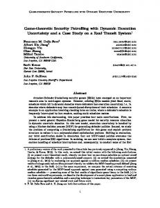
L EMMA 1. For all coupled randomized policy π, the resulting marginal probabilities wi (si , ai ) and xi (si , ai , s0i ) satisfy constraints (4), (5), (6), (7). P ROOF S KETCH . Constraint (4) holds by the definition of transition probabilities of MDPs. Constraint (5) holds because both lhs and rhs equal the marginal probability of reaching state s. Constraint (6) holds because by construction, the marginal probability of reaching s+ i is 1, and so is the marginal probability of reaching s− i . Constraint (7) holds because wi (si , ai ) is a probability. Intuitively, if we can formulate utilities in terms of w and x, which have dimensions polynomial in the sizes of the MDPs, this will lead to a much more compact representation of the SSE problem compared to (1). It turns out this is possible if the game’s utilities are separable, which intuitively means that given the adversary’s strategy, the utilities of both players are sums of contributions from individual units’ individual transitions: D EFINITION 1. A patrolling game with execution uncertainty as defined in Section 2.2 has separable utilities if there exist utilities Uλd (si , ai , s0i , α) and Uλa (si , ai , s0i , α) for each unit i, transition (si , ai , s0i ), λ ∈ Λ, α ∈ A, such that for all t ∈ X , λ ∈ Λ, α ∈ A, the defender’s P andP the adversary’s utilities can be expressed as ud (t, λ, α) = i si ,ai ,s0 θ(ti , si , ai , s0i )Uλd (si , ai , s0i , α) i P P 0 a 0 and ua (t, λ, α) = i si ,ai ,s0i θ(ti , si , ai , si )Uλ (si , ai , si , α), respectively. Let Uλd , Uλa ∈ RM ×|A| be the corresponding matrices. Then Uλd , Uλa completely specifies the utility functions ud and ua . τ0 L1
L1, τ0
τ1 1.0
Stay
L1, τ1
τ2
0.9 0.9
0.9 To L1
0.1
0.1 Stay
L1, τ2
0.1 To L2
0.9
To L1 L2, τ0
1.0
Stay
0.1 To L2
L2
3.1
(3)
t∈X
1.0
L2, τ1
Stay
1.0
L2, τ2
Figure 1: Example game with separable utilities.
E XAMPLE 1. Consider the following simple example game with one defender unit, whose MDP is illustrated in Figure 1. There are six states, shown as circles in the figure, over two locations L1 , L2 and three time points τ0 , τ1 , τ2 . From states at τ0 and τ1 , the unit has two actions: to stay at the current location, which always succeeds, and to try to go to the other location, which with probability 0.9 succeeds and with probability 0.1 fails (in which case it stays at the current location). There are 12 transitions in total, which is fewer than the number of complete trajectories (18). There is a single type of adversary who chooses one location between L1 and L2 and one time point between τ1 and τ2 to attack (τ0 cannot be chosen). If the defender is at that location at that time, the attack fails and both players get zero utility. Otherwise, the attack succeeds, and the adversary gets utility 1 while the defender gets −1. In other words, the attack succeeds if and only if it avoids the defender unit’s trajectory. It is straightforward to verify that this game has separable utilities: for any transition (si , ai , s0i ) in the MDP, let Uλa (si , ai , s0i , α) be 1 if α coincides with s0i and 0 otherwise. For example, the utility expression for the adversary given trajectory ((L1 , τ0 ), To L2 , (L1 , τ1 ), To L2 , (L2 , τ2 )) is Uλa ((L1 , τ0 ), To L2 , (L1 , τ1 ), α)+Uλa ((L1 , τ1 ), To L2 , (L2 , τ2 ), α), which gives the correct utility value for the adversary: 1 if α equals (L1 , τ1 ) or (L2 , τ2 ) and 0 otherwise. It is straightforward to show the following. L EMMA 2. Consider a game with separable utilities. Suppose x is the vector of marginal probabilities induced by the defender’s randomized policy π. Let yλ ∈ R|A| be a vector describing the mixed strategy of the adversary of type λ, with yλ (α) denoting the probability of choosing action α. Then the defender’sPand the adversary’s expected utilities from their interactions are λ pλ xT Uλd yλ P and λ pλ xT Uλa yλ , respectively. In other words, given the adversary’s strategy, the expected utilities of both players are linear in the marginal probabilities xi (si , ai , s0i ). Lemma 2 also applies when (as in an SSE) the adversary is playing a pure strategy, in which case yλ is a 0-1 integer vector with yλ (α) = 1 if α is the action chosen. We can thus use this compact representation of defender strategies to rewrite the formulation for SSE (1) as a polynomial-sized optimization problem.
max
w,x,y
X
pλ xT Uλd yλ +
γ X X
xi (si , ai , s0i )Ri (si , ai , s0i ) (8)
i=1si ,ai ,s0 i
λ∈Λ
s.t. constraints (4), (5), (6), (7) X yλ (α) = 1, yλ (α) ∈ {0, 1}
(9)
α
yλ ∈ arg max xT Uλa yλ0 0
(10)
yλ
As we will show in Section 3.2, given a solution w, x to (8), we can calculate a decoupled policy that matches the marginals w, x. Compared to (1), the optimization problem (8) has exponentially fewer dimensions; in particular the numbers of variables and constraints are polynomial in the sizes of the MDPs. Furthermore, existing methods for solving Bayesian Stackelberg games can be directly applied to (8) such as mixed-integer linear program formulation [8] or branch-and-bound [14]. For the special case of Uλd + Uλa = 0 for all λ, i.e., when the interaction between defender and adversary is zero-sum, the above
SSE problem can be formulated as a linear program (LP) X X X max pλ uλ + xi (si , ai , s0i )Ri (si , ai , s0i ) w,x,u
λ∈Λ
i
(11)
si ,ai ,s0i
s.t. constraints (4), (5), (6), (7) uλ ≤ xT Uλd eα , ∀λ ∈ Λ, α ∈ A,
(12)
where eα is the basis vector corresponding to adversary action α. This LP is similar to the maximin LP for a zero-sum game with the utilities given by Uλd and Uλa , except that an additional term P P 0 0 i si ,ai ,s0i xi (si , ai , si )Ri (si , ai , si ) representing defender’s expected utilities from immediate rewards is added to the objective. One potential issue arises: because of the extra defender utilities from immediate rewards, the entire game is no longer zero-sum. Is it still valid to use the above maximin LP formulation? It turns out that the LP is indeed valid, as the immediate rewards do not depend on the adversary’s strategy. P ROPOSITION 1. If the game has separable utilities and Uλd + = 0 for all λ, then a solution of the LP (11) is an SSE.
Uλa
P ROOF S KETCH . We can transform this game to an equivalent zero-sum Bayesian game whose LP formulation is equivalent to (11). Specifically, given the non-zero-sum Bayesian game Γ specified above, consider the Bayesian game Γ0 with the following “meta” type distribution for the second player: for all λ ∈ Λ of Γ there is a corresponding type λ0 ∈ Λ0 in Γ0 , with probability pλ0 = 0.5pλ , with the familiar utility functions; and there is a special type φ ∈ Λ0 with probability pφ = 0.5, whose action does not affect either player’s utility. Specifically φ P P the utilities under0 the special type 0 θ(t , s , a , s )R (s , a , s ) and are ud (t, φ, α) = 0 i i i i i i i i i si ,ai ,si P P ua (t, φ, α) = − i si ,ai ,s0 θ(ti , si , ai , s0i )Ri (si , ai , s0i ). The i resulting game Γ0 is zero-sum, with the defender’s utility exactly half the objective of (11). Since for zero-sum games maximin strategies and SSE coincide, a solution of the LP (11) is an optimal SSE marginal vector for the defender of Γ0 . On the other hand, if we compare the induced normal forms of Γ and P Γ0 , the only difference is that for the adversary the utility −0.5 e∈E ∗ Ue xe is added, which does not depend on the adversary’s strategy. Therefore Γ and Γ0 have the same set of SSE, which implies that a solution of the LP is an SSE of Γ.
3.2
Generating Patrol Schedules
The solution of (8) does not yet provide a complete specification of what to do. We ultimately want an explicit procedure for generating the patrol schedules. We define a Markov strategy π to be a decoupled strategy (π1 , . . . , πγ ), πi : Si × Ai → R, where the distribution over next actions depends only on the current state. Proposition 2 below shows that given w, x, there is a simple procedure to calculate a Markov strategy that matches the marginal probabilities. This implies that if w, x is the optimal solution of (8), then the corresponding Markov strategy π achieves the same expected utility. We have thus shown that for games with separable utilities it is sufficient to consider Markov strategies. P ROPOSITION 2. Given w, x satisfying constraints (4) to (7), construct a Markov strategy π as follows: for each si ∈ Si , for (si ,ai ) each ai ∈ Ai (si ), πi (si , ai ) = P w0iw 0 . Suppose the dei (si ,a ) a
i
i
fender plays π, then for all unit i and transition (si , ai , s0i ), the probability that (si , ai , s0i ) is reached by i equals xi (si , ai , s0i ). P ROOF S KETCH . Such a Markov strategy π induces a Markov chain over the states Si for each unit i. It can be verified by induction that the resulting marginal probability vector matches x.
In practice, directly implementing a Markov strategy requires the unit to pick an action according to the randomized Markov strategy at each time step. This is possible when units can consult a smartphone app that stores the strategy, or can communicate with a central command. However, in certain domains such requirement on computation or communication at each time step places additional logistical burden on the patrol unit. To avoid unnecessary computation or communication at every time step, it is desirable to have a deterministic schedule (i.e., a pure strategy) from the Markov strategy. With no execution uncertainty, a pure strategy can be specified by the a complete trajectory for each unit. However, this no longer works in the case with execution uncertainty. We thus begin by defining a Markov pure strategy, which specifies a deterministic choice at each state.
1 a non-default transition takes unit 1 to location LA at time 3. We modify unit 1’s MDP so that this transition ends at a new state (L1A , 2) ∈ S1 , where L1A is a “special” location specifying that the unit will become alive again at location LA in one more time step. There is only one action from (L1A , 2), with only one possible next state (LA , 3). Once we have modified the individual units’ MDPs so that all transitions take exactly one time step, we can create the Cartesian Product MDP as described in the previous paragraph. Like the units’ MDPs, the Cartesian Product MDP is also acyclic. Therefore we can analogously define marginal probabilities w× (s× , a× ) and x× (s× , a× , s0× ) on the Cartesian Product MDP. Let w× ∈ 2 R|S× ||A× | and x× ∈ R|S× | |A× | be the corresponding vectors. Utilities generally cannot be expressed in terms of w× and x× . We consider a special case in which utilities are partially separable:
D EFINITION 2. A Markov pure strategy q is a tuple (q1 , . . . , qγ ) where for each unit i, qi : Si → Ai .
D EFINITION 3. A patrolling game with execution uncertainty has partially separable utilities if there exist Uλd (s× , a× , s0× , α) and Uλa (s× , a× , s0× , α) for each transition (s× , a× , s0× ), λ ∈ Λ, α ∈ A, such that for all t ∈ X , λ ∈ Λ, α ∈ A, the defender’s and as ud (t, λ, α) = P the adversary’s utilities0 cand be expressed 0 a s ,a ,s0 θ× (t, s× , a× , s× )Uλ (s× , a× , s× , α) and u (t, λ, α) = P× × × 0 0 a s× ,a× ,s0 θ× (t, s× , a× , s× )Uλ (s× , a× , s× , α), respectively.
Given a Markov strategy π, we sample a Markov pure strategy q as follows: for each unit i and state si ∈ Si , sample an action ai as qi (si ) according to πi . This procedure is correct since each state in i’s MDP is visited at most once and thus qi exactly simulates a walk from s+ i on the Markov chain induced by πi . To directly implement a Markov pure strategy, the unit needs to remember the entire mapping q or receives the action from the central command at each time step. A logistically more efficient way is for the central command to send the unit a trajectory assuming perfect execution, and only after a non-default transition happened does the unit communicates with the central command to get a new trajectory starting from the current state. Formally, given si ∈ Si and qi , we define the optimistic trajectory from si induced by qi to be (si , qi (si ), n(si , qi (si )), . . . s− ), i.e, the trajectory assuming it always reaches its default next state. Given a Markov pure strategy q, the following procedure for each unit i exactly simulates q: (i) central command gives unit i the optimistic trajectory from s+ induced by qi ; (ii) unit i follows the trajectory until the terminal state s− is reached or some unexpected event happens and takes i to state s0i ; (iii) central command sends the new optimistic trajectory from s0i induced by qi to unit i and repeat from step (ii).
3.3
×
Partially separable utilities is a weaker condition than separable utilities, as now the expected utilities may not be sums of contributions from individual units. When utilities are partially separable, we can express expected utilities in terms of w× and x× and find an SSE by solving an optimization problem analogous to (8). From ∗ ∗ the optimal w× , we can get a Markov strategy π× (s× , a× ) = w∗ (s× ,a× ) P × ∗ , 0 a0 w× (s,a× )
This approach cannot scale up to a large number of defender units, as the size of S× and A× grow exponentially in the number of units. In particular the dimension of the Markov policy π× is already exponential in the number of units. To overcome this we will need a more compact representation of defender strategies. One approach is to use decoupled strategies. Although no longer optimal in general, we will see in Section 3.4 that this approach gives a good approximation in the LA Metro domain.
Coupled Execution: Cartesian Product MDP 3.4
Without the assumption of separable utilities, it is no longer sufficient to consider decoupled Markov strategies of individual units’ MDPs. We create a new MDP that captures the joint execution of patrols by all units. For simplicity of exposition we look at the case with two defender units. Then a state in the new MDP corresponds to the tuple (location of unit 1, location of unit 2, time). An action in the new MDP corresponds to a tuple (action of unit 1, action of unit 2). Formally, if unit 1 has an action a1 at state s1 = (l1 , τ ) that takes her to s01 = (l10 , τ 0 ) with probability T1 (s1 , a1 , s01 ), and unit 2 has an action a2 at state s2 = (l2 , τ ) that takes her to s02 = (l20 , τ 0 ) with probability T2 (s2 , a2 , s02 ), we create in the new MDP an action a× = (a1 , a2 ) from state s× = (l1 , l2 , τ ) that transitions to s0× = (l10 , l20 , τ 0 ) with probability T× (s× , a× , s0× ) = T1 (s1 , a1 , s01 )T2 (s2 , a2 , s02 ). The immediate rewards R× of the MDP are defined analogously. We call the resulting MDP (S× , A× , T× , R× ) the Cartesian Product MDP. An issue arises when at state s× the individual units have transitions of different time durations. For example, unit 1 rides a train that takes 2 time steps to reach the next station while unit 2 stays at a station for 1 time step. During these intermediate time steps only unit 2 has a “free choice”. How do we model this on the Cartesian Product MDP? One approach is to create new states for the intermediate time steps. For example, suppose at location LA at time
which is provably the optimal coupled strategy.
×
Application to LA Metro Domain
We now explain how our proposed techniques can be used in the LA Metro domain. As we will see, although the utilities in this domain are not separable, we are able to upper bound the defender utilities by separable utilities, allowing efficient computation. Similar to [13], a state here comprises the current station and time of a unit, as well as necessary history information such as starting time1 . At any state, a unit may stay at her current station to conduct an in-station operation for some time or she can ride a train to conduct an on-train operation when her current time coincides with the train schedule. Due to execution uncertainty, a unit may end up at a state other than the intended outcome of the action. For ease of analysis, we assume throughout a single type of unexpected event which delays a patrol unit for some time beyond the intended execution time. Specifically, we assume for any fare check operation taken, there is a probability η that the operation will be delayed, i.e., staying at the same station (for in-station operations) or on the same train (for on-train operations) involuntarily for some time. Furthermore, we assume that units will be involved with events unrelated to fare enforcement and thus will not check fares during any delayed period of an operation. Intuitively, a higher chance of delay leads to less time spent on fare inspection. 1
Interested readers are encouraged to read [13] for more details
The adversary faced here are the riders in the system. There are multiple types of riders, each is assumed to take a fixed route. A rider observes the likelihood of being checked and makes a binary decision between buying and not buying the ticket. If the rider of type λ buys the ticket, he pays a fixed ticket price ρλ . Otherwise, he rides the train for free but risks the chance of being caught and paying a fine of %λ > ρλ . The LASD’s objective is set to maximize the overall revenue of the whole system including ticket sales and fine collected, essentially forming a zero-sum game. Since the fare check operation performed is determined by the actual transition rather than the action taken, we define the effectiveness of a transition (s, a, s0 ) against a rider type λ, fλ (s, a, s0 ), as the percentage of riders of type λ checked by transition (s, a, s0 ). Following the same argument as in [13], we assume the probability that a joint complete trajectory t detects evader λ as the sum of fλ over all transitions in t = (t1 , . . . , tγ ) capped at one: Pr(t, λ) = min{
γ X X
4.
For type λ and joint trajectory t, the LASD receives ρλ if the rider buys the ticket and %λ · Pr(t, λ) otherwise. The utilities in this domain are indeed not separable — even though multiple units (or even a single unit) may detect a fare evader multiple times, the evader can only be fined once. As a result, neither players’ utilities can be computed directly using marginal probabilities x and w. Instead, we upper bound the defender utility by overestimating the detection probability using marginals as the following: γ X X
fλ (si , ai , si )xi (si , ai , s0i ).
(14)
i=1 si ,ai ,s0 i
Equation (14) leads to the following upper bound LP for the LA Metro problem: X
max
x,w,u
pλ uλ +
γ X X
Ri (si , ai , s0i )
(15)
i=1 si ,ai ,s0 i
λ∈Λ
Intuitively, LP (15) relaxes the utility functions by allowing an evader to be fined multiple times during a single trip. The relaxed utilities are separable and thus the relaxed problem can be efficiently solved. Since the solution returned x∗ and w∗ satisfy constraints (4) to (7), we can construct a Markov strategy from w∗ as described in Section 3.2. The Markov strategy provides an approximate solution to the original problem, whose actual value can be evaluated using Monte Carlo simulation.
fλ (si , ai , s0i )θ(ti , si , ai , s0i ), 1}. (13)
i=1 si ,ai ,s0 i
\λ) = Pr(x,
P ROOF S KETCH . Let x∗ and w∗ be the marginal coverage and be the value of the patroller against rider type λ in the optimal coupled strategy π ∗ . It suffices to show that x∗ , w∗ , and u∗ is a feasible point of the LP. From Lemma 1, we already know x∗ and w∗ must satisfy constraints (4) to (7). Furthermore, we have u∗λ ≤ ρλ since the rider pays at most the ticket price. Finally, \λ) since Pr(x, \λ) is an overestimate of the true u∗λ ≤ %λ · Pr(x, detection probability. u∗λ
s.t. constraints (4), (5), (6), (7) \λ)}, for all λ ∈ Λ uλ ≤ min{ρλ , %λ · Pr(x,
(16)
We prove the claims above by the following two propositions.
4.1
Line Red Blue Gold Green
P ROOF S KETCH . Consider a coupled strategy π. Recall that ϕ(t; π) ∈ R is the probability that joint trajectory t ∈ X is instantiated. For rider type λ, the true detection probability is Pr(π, λ) = P t∈X ϕ(t; π)Pr(t, λ). Applying Equations (13) and (3) we have, X
ϕ(t; π)
γ X X i=1 si ,ai ,s0 i
=
γ X X i=1
Stops
Trains
Daily Riders
Types
16 22 19 14
433 287 280 217
149991.5 76906.2 30940.0 38442.6
26033 46630 41910 19559
Table 1: Statistics of Los Angeles Metro lines.
fλ (si , ai , s0i )θ(ti , si , ai , s0i )
i=1 si ,ai ,s0 i
t∈X
=
γ X X
Data Sets
We used the same four data sets as in [13], each based on a different Los Angeles Metro Rail line: Red (including Purple), Blue, Gold, and Green. In these data sets, the train schedules were obtained from http://www.metro.net and the ridership distributions were estimated from hourly boarding and alighting counts provided by the LASD. We allowed any on-train operations while restricted in-station operations to be between half an hour and an hour, as suggested by the LASD. The effectiveness of each fare check operation was adjusted based on the volume of riders during the period with an assumption that a unit can check three riders per minute. Same as in [13], The ticket fare was set to $1.5 while the fine was set to $100. The immediate rewards Ri are all set to zero. Table 1 summarizes the detailed statistics for the four Metro lines.
\λ) is an upper bound of the true detecP ROPOSITION 3. Pr(x, tion probability of any coupled strategy with marginals x.
Pr(π, λ) ≤
EVALUATION
We present our evaluation based on real metro schedules and rider traffic data provided by the LASD. We solved LP (15) using CPLEX 12.2 with the barrier method on standard 2.8GHz machines with 4GB memory. Each Markov strategy induced from the LP solution was evaluated using Monte Carlo simulation with 100, 000 samples. Riders were assumed to choose a best response based on the frequency of being checked over these samples. We first describe the data sets we used, followed by our experimental results.
fλ (si , ai , s0i )
X
ϕ(t; π)θ(ti , si , ai , s0i )
t∈X
\λ). fλ (si , ai , s0i )xi (si , ai , s0i ) = Pr(x,
si ,ai ,s0i
P ROPOSITION 4. LP (15) provides an upper bound of the optimal coupled strategy.
4.2
Experimental Results
We studied the performance of our Markov strategies under a variety of settings. Throughout the settings that we have tested, we found that the Markov strategy was close to optimal with revenue always above 99% of the LP upper bound. In the remainder of this subsection we will report values of the Markov strategy without mentioning the LP upper bound. Given space limits, in some cases, we have only presented results for the Red line, but other lines were also tested and showed similar results.
0.3
Markov Arbitrary Abort
0 0 0.05 0.1 0.15 0.2 0.25 Probability of unexpected event
Fare evasion rate
20%
Blue
Gold
Green
Markov Arbitrary Abort
0.3 0 5
10
15 20 Delay time
25
(b) Markov strategy vs. pre-generated strategy (varying delay time) Red
15% 10% 5% 0% 0 0.05 0.1 0.15 0.2 0.25 Probability of unexpected event
(e) Evasion rate of Markov strategy
(c) Markov strategy vs. pre-generated strategy (evasion rate)
1.5 Revenue per rider
(a) Markov strategy vs. pre-generated strategy (varying η)
0.6
Low
Medium
High
1.1 0.9 0.7 0 0.05 0.1 0.15 0.2 0.25 Probability of unexpected event
(f) Revenue decay with varying coverage levels
1.2 1
η = 0% η = 10% η = 20%
0.8 0.6 2
3 4 5 Number of patrol units
(g) Revenue per rider with increasing coverage
1.45 1.4 1.35 Blue
Gold
Green
Red
1.3 0 0.05 0.1 0.15 0.2 0.25 Probability of unexpected event
(d) Revenue per rider of Markov strategy
1.4
1.3
1.5 Revenue per rider
0.6
0.9
1 0.9 0.8 0.7 0.6 0.5 Markov 0.4 Arbitrary 0.3 Abort 0.2 0.1 0 0.05 0.1 0.15 0.2 0.25 Probability of unexpected event
Runtime(in minutes)
0.9
1.2
Revenue per rider
1.2
Fare evasion rate
1.5 Revenue per rider
Revenue per rider
1.5
6
60 Blue 54 48 Gold 42 Green 36 Red 30 24 18 12 6 0 0 0.05 0.1 0.15 0.2 0.25 Probability of unexpected event
(h) Worst-case LP runtime
Figure 2: Experimental results.
In the first set of experiments, we compared, under execution uncertainty, the performance of our Markov strategy against pregenerated schedules given by TRUSTS, a deterministic model assuming perfect execution. However, actions to take after deviations from the original plan are not well-defined in TRUSTS schedules, making a direct comparison inapplicable. Therefore, we augmented these pre-generated schedules with two naive contingency plans indicating the actions to follow after a unit deviates from the original plan. The first plan, “Abort”, is to simply abandon the entire schedule and return to the base. The second plan, “Arbitrary”, is to pick an action uniformly randomly from all available actions at any decision point after the deviation. In this experiment, we fixed the number of units to 6 and the patrol length to 3 hours, and presented the results on the Red line (experiments on other lines showed similar results). We first fixed the delay time to 10 minutes and varied the delay probability η from 0% to 25%. As we can see in Figure 2(a), both “Abort” and “Arbitrary” performed poorly in the presence of execution uncertainty. With increasing values of η, the revenue of “Abort” and “Arbitrary” decayed much faster than the Markov strategy. For example, when η was increased from 0% to 25%, the revenue of “Abort” and “Arbitrary” decreased 75.4% and 37.0% respectively while that of the Markov strategy only decreased 3.6%. In addition to revenue, Figure 2(c) showed the fare evasion rate of the three policies with increasing η. Following the same definition in [13], we considered a rider to prefer fare evasion if and only if his expected penalty from fare evasion is $0.2 lower than $1.5, the ticket price. As we can see, “Abort” and “Arbitrary” showed extremely poor performance in evasion deterrence with even a tiny probability of execution error. In particular, when η was increased from 0% to 5%, the evasion rate of the Markov strategy barely increased while that of “Abort” and “Arbitrary” increased from 11.2% both to 74.3% and 43.9% respectively. Then we fixed η to 10% and varied the delay time from 5 to 25 minutes. Figure 2(b) showed that both “Abort” and “Arbitrary” performed worse than the Markov strategy. With increasing delay time, the revenue of “Abort” remained the same as the time of the
delay really did not matter if the unit was to abandon the schedule after the first unexpected event. The revenue of “Arbitrary”, however, decayed in a faster rate than the Markov strategy. When the delay time was increased from 5 to 25 minutes, the revenue of “Abort” remained the same while that of “Arbitrary” and the Markov strategy decreased 14.4% and 3.6% respectively. An important observation here is that the revenue of “Abort”, a common practice in fielded operations, decayed extremely fast with increasing η — even with a 5% probability of delay, the revenue of “Abort” was only 73.5% of that of the Markov strategy. With a conservative estimate of 6% potential fare evaders [4] and 300, 000 daily riders in the LA Metro Rail system, the 26.5% difference implies a daily revenue loss of $6, 500 or $2.4 million annually. In the second set of experiments, we showed that the Markov strategy performed well consistently in all of the four lines with increasing delay probability η. We fixed the number of units to 6 and the patrol length to 3 hours, but varied η from 0% to 25%. Figure 2(d) and Figure 2(e) showed the revenue per rider and the evasion rate of the four lines respectively2 . As we can see, the revenue decreased and the evasion rate increased with increasing η. However, the Markov strategy was able to effectively allocate resources to counter the effect of increasing η in terms of both revenue maximization and evasion deterrence. For example, the ratio of the revenue of η = 25% to that of η = 0% was 97.2%, 99.1%, 99.9%, 95.3% in the Blue, Gold, Green and Red line respectively. Similarly, when η was increased from 0% to 25%, the evasion rate of the Blue, Gold, Green and Red line was increased by 4.6, 1.9, 0.1, 5.2 percentage points respectively. Our next experiment showed that the revenue decay of the Markov strategy with respect to delay probability η could be affected by the amount of resources devoted to fare enforcement. In Figure 2(f), we presented the revenue per rider with increasing η on the Red line only, but the same trends were found on the other three lines. 2
The revenue of the Red line was significantly lower than the other lines because fare check effectiveness fλ defined in Section 3.4 was set inversely proportional to the ridership volume.
In this experiment, we considered 3, 6 and 9 patrol units, representing three levels of fare enforcement: low, medium, and high respectively. Intuitively, with more resources, the defender could better afford the time spent on handling unexpected events without sacrificing the overall revenue. Indeed, as we can see, the rate of revenue decay with respect to η decreased as we increased the level of fare enforcement from low to high. For example, when η was increased from 0% to 25%, the revenue drop in the low, medium and high enforcement setting was 13.2%, 4.7%, and 0.4% respectively. Next, we demonstrate the usefulness of our Markov strategy in distributing resources under different levels of uncertainty. We showed results on the Red line with a fixed patrol length of 3 hours. Three delay probabilities η = 0%, 10%, and 20% were considered, representing increasing levels of uncertainty. Figure 2(g) showed the revenue per rider with increasing number of units from 2 to 6. As we increased the number of units, the revenue increased towards the maximal achievable value of $1.5 (ticket price). For example, when η = 10%, the revenue per rider was $0.65, $1.12, and $1.37 with 2, 4, and to 6 patrol units respectively. Finally, Figure 2(h) plotted the worst-case runtime (over 10 runs) of the LP with increasing η for the four metro lines. The number of units was fixed to 3 and the patrol length per unit was fixed to 3 hours. As we can see, we were able to solve all of the problems within an hour. The runtime varied among the four Metro lines and correlated to their number of states and types. For example, when η = 10%, the runtime for the Blue, Gold, Green, and Red line was 14.0, 24.3, 2.4, and 4.3 minutes respectively. Surprisingly, for all of the four lines, stochastic models with η = 5% took less time to solve than deterministic models (η = 0%). Overall we found no direct correlation between the runtime and delay probability η.
5.
CONCLUSION AND RELATED WORK
This paper addresses dynamic execution uncertainty in scheduling security and law-enforcement patrols in time-critical domains. We propose a general Stackelberg game model for security patrolling with execution uncertainty, and show that efficient computation of SSE is possible when utilities have separable structure. We apply our approach to fare inspection in the Los Angeles Metro Rail system. Numerical experiments show that our approach outperform schedules generated using the previous TRUSTS algorithm, which does not consider execution uncertainty. There has been significant research on uncertainty modeling and robust strategy computation in leader-follower Stackelberg games, including robust optimization [12], sample average approximation [14], equilibrium refinement [1], and human adversary modeling [11]. These works focused on one shot games in which the defender’s pure strategy is a single action. Our model resembles the transition independent DEC-MDP [3], where coupled and decoupled execution correspond to the case with and without communication respectively. However, two major distinctions exist, presenting unique computational challenges. First, we consider the strategic interaction against adversaries and focus on equilibrium computation. Second, utility functions in our model are non-Markovian which depend on trajectories as opposed to only state and action pairs in typical DEC-MDP models. The game model in this paper can be considered as a special case of extensive-form Stackelberg games with chance nodes, or as a special case of stochastic Stackelberg games where the follower can only choose one action in the initial state and stick to that action in all future states. The general cases of both games were shown to be NP-hard [6, 7]. Vorobeychik and Singh provided mixed integer linear programs for finding optimal and approximate Markov stationary strategy in general-sum stochastic Stackelberg games [10].
However, their approach does not handle multiple adversary types and their MILP formulation lacks the scalability to a large number of states such as the LA Metro problems. Another related line of research is on equilibrium refinement for dynamic games, such as trembling hand perfect equilibrium [2], which considers the possibility that a strategy can be imperfectly executed. However such research is mainly interested in the limit as uncertainty goes to zero, while in our real world settings the probability of imperfect execution really is non-zero.
6.
ACKNOWLEDGEMENT
We thank the Los Angeles Sheriff’s Department for their exceptional collaboration. This research is supported by TSA grant HSHQDC-10-A-BOA19, MURI grant W911NF-11-1-0332, the Google Inter-university Center for Electronic Markets and Auctions and MOST 3-6797.
7.
REFERENCES
[1] B. An, M. Tambe, F. Ordonez, E. Shieh, and C. Kiekintveld. Refinement of strong Stackelberg equilibria in security games. In AAAI, 2011. [2] M. Aoyagi. Reputation and dynamic Stackelberg leadership in infinitely repeated games. Journal of Economic Theory, 71(2):378 – 393, 1996. [3] R. Becker, S. Zilberstein, V. Lesser, and C. V. Goldman. Solving Transition Independent Decentralized Markov Decision Processes. JAIR, 2004. [4] Booz Allen Hamilton. Faregating analysis. Report commissioned by the LA Metro, http://boardarchives.metro.net/Items/2007/11_ November/20071115EMACItem27.pdf, 2007.
[5] V. Conitzer and T. Sandholm. Computing the optimal strategy to commit to. In EC: Proceedings of the ACM Conference on Electronic Commerce, 2006. [6] J. Letchford and V. Conitzer. Computing optimal strategies to commit to in extensive-form games. In EC, 2010. [7] J. Letchford, L. MacDermed, V. Conitzer, R. Parr, and C. L. Isbell. Computing optimal strategies to commit to in stochastic games. In AAAI, 2012. [8] P. Paruchuri, J. P. Pearce, J. Marecki, M. Tambe, F. Ordonez, and S. Kraus. Playing games with security: An efficient exact algorithm for Bayesian Stackelberg games. In AAMAS, 2008. [9] M. Tambe. Security and Game Theory: Algorithms, Deployed Systems, Lessons Learned. Cambridge University Press, 2011. [10] Y. Vorobeychik and S. Singh. Computing stackelberg equilibria in discounted stochastic games. In AAAI, 2012. [11] R. Yang, F. Ordonez, and M. Tambe. Computing optimal strategy against quantal response in security games. In AAMAS, 2012. [12] Z. Yin, M. Jain, M. Tambe, and F. Ordonez. Risk-averse strategies for security games with execution and observational uncertainty. In AAAI, 2011. [13] Z. Yin, A. X. Jiang, M. P. Johnson, M. Tambe, C. Kiekintveld, K. Leyton-Brown, T. Sandholm, and J. Sullivan. TRUSTS: Scheduling randomized patrols for fare inspection in transit systems. In IAAI, 2012. [14] Z. Yin and M. Tambe. A unified method for handling discrete and continuous uncertainty in Bayesian Stackelberg games. In AAMAS, 2012.