Hindawi Publishing Corporation International Journal of Distributed Sensor Networks Volume 2014, Article ID 572524, 13 pages http://dx.doi.org/10.1155/2014/572524
Research Article Game Theoretic Request Scheduling with Queue Priority in Video Sensor Networks Jia Zhao,1 Jianfeng Guan,2 Changqiao Xu,2,3 and Wei Su1 1
National Engineering Laboratory for Next Generation Internet Interconnection Devices, Beijing Jiaotong University, Beijing 100044, China 2 State Key Laboratory of Networking and Switching Technology, Beijing University of Posts and Telecommunications, Beijing, China 3 Institute of Sensing Technology and Business, Beijing University of Posts and Telecommunications, Wuxi, Jiangsu, China Correspondence should be addressed to Jia Zhao;
[email protected] Received 1 November 2013; Accepted 8 February 2014; Published 30 March 2014 Academic Editor: Hongke Zhang Copyright © 2014 Jia Zhao et al. This is an open access article distributed under the Creative Commons Attribution License, which permits unrestricted use, distribution, and reproduction in any medium, provided the original work is properly cited. Video sensor networks have been widely used to monitor environment and report abnormality. Each node collects video data, select a head node, and transmit the data to the head, and then the head reports the data to the base station. A head has to process both normal and abnormal data-reporting requests from its nearby nodes. To achieve QoS of surveillance, previous request scheduling methods minimize the data transmission delay or blocking rate but no comprehensive way was studied in the literature. In this paper, we propose a game strategic request scheduling based on a queue priority model in which a handover mechanism ensures that the abnormal requests are processed in time. In the game, video sensors select their heads to decide the arriving rates of both normal and abnormal requests; the heads decide the probability of handing over the abnormal requests. At the Nash Equilibrium Point (NEP), the normal data requesters optimize mean delay, the abnormal data requesters optimize mean blocking rate, and the heads balance the request load on them. Numerical analysis shows that the game strategic scheduling outperforms other scheduling methods that consider single objective (minimum delay or minimum blocking rate).
1. Introduction Video sensor networks act as an efficient and reliable way to monitor environment and discover emergency or accidents [1, 2]. Each node of a sensor network collects video data and transmits the data to a nearby head, which is also a sensor and selected within a cluster. The head processes the datareporting requests from members of the cluster and transmits the data to a sink node or a base station. The monitoring quality of service (QoS) of a video sensor network depends on how the data-reporting requests are scheduled and processed [2]. In order to collect data in time, a scheduling mechanism is supposed to optimize a metric of QoS (e.g., delay or blocking rate). When executing the task of surveillance, a video sensor node can provide two types of service, one of which is to collect the data of normal video stream, and the other one is to collect the data of accident identification. Compared with
the normal data, the abnormal data has a strict requirement of real time in order that the emergency and accidents can be discovered in time. A sensor node may transmit either normal or abnormal data to heads, which have to process both kinds of requests. Accordingly, a scheduling mechanism has to be designed to ensure that regular monitoring tasks are accomplished and accident reports are not delayed. Previous request scheduling mechanisms focused on optimizing a single QoS metric (e.g., delay or blocking rate) without considering different QoS demands of two kinds of requests. Some work deals with packet queue management to improve the reporting delay and the video distortion [3]. Some other work pays too much attention to the occasionally accident data to avoid disturbing the regular monitoring tasks [4, 5]. A comprehensive way to achieve QoS of both kinds of reporting requests has not been studied in the literature. Such request scheduling problem entails a solution to optimize the utility of both the normal data-reporting requesters and
2 abnormal data-reporting requesters. Game theory can be used where multiple participants interact with each other by their own strategies and pursue their respective optimal utility. When the participants arrive a Nash Equilibrium Point, they will not deviate from this solution because no more profit can be achieved by any of them [6, 7]. During the transmission of normal and abnormal data, there are totally three active participants: abnormal data-reporting requesters (ADR), normal data-reporting requesters (NDR), and cluster heads. They interact with each other. Both ADR and NDR have to choose the right heads to report their data because their choices will influence QoS of their monitoring tasks and the performance of the whole network. The cluster heads have to use cooperative way to optimize the cost and prolong the lifetime of the network. The three participants optimize their respective utility objective and converge to an equilibrium at which ADR and NDR make optimal head selection and heads use cooperation mechanism to lower and balance load on them. In this paper, we propose a game theoretic request scheduling based on a handover mechanism between heads’ priority queues. ADR, NDR, and the heads act as three players in the game. NDR decides the head selection strategy to optimize mean request response delay. ADR selects their heads to optimize mean request blocking rate. The Cluster heads decide the handover strategy to optimize their load. We can get a Nash Equilibrium Point (NEP) at which each participant optimizes its own utility [6, 7]. Using NEP solution as the request scheduling, we satisfy the demand of service quality of both ADR and NDR as well as achieving load balance between heads. The main contributions of this paper include the following: (1) we analyze the interaction among the three active participants in request scheduling game and aim to converge their respective behaviors (strategies) to an optimal equilibrium; (2) from the view of data-reporting requesters, we use a comprehensive way to optimize utility of both kinds of data-reporting requesters rather than pay too much attention to a single QoS metric; (3) from the view of cluster heads, we propose a handover mechanism between their request queue with priority in order to balance their respective load and prolong the lifetime. The remainder of the paper is organized as follows. Related work is introduced in Section 2. In Section 3, we illustrate the network and QoS metrics. In Section 4 we propose the request scheduling game and the NEP solution. Some properties of NEP are validated in Section 5. Evaluation of the scheduling is shown in Section 6. Section 7 concludes the paper.
2. Related Work In video sensor networks, abnormal data-reporting requests are usually given the high priority for accident discovery. In the paper [4], the authors propose an energy-aware packet scheduling algorithm to minimize the power consumption and prolong the lifetime of the whole video sensor network. In order to minimize the video distortion, they use a priority strategy to let the high priority packets to be transmitted
International Journal of Distributed Sensor Networks over high bandwidth paths. Their proposed algorithm can constrain the energy consumption by selectively dropping the least important video packets. Durmus et al. propose an event-based fairness scheme for fair resource allocation of the involving events [3]. Their scheme is a queue management to improve the video distortion and the reporting latency. In the paper [5], the authors propose a periodic time scheduling to maximize the quality of monitoring of stochastic events. This scheduling has to decide the proportion of the time of eventmonitoring and distribute a sensor’s coverage time in order to achieve the proportion sharing and prolong the lifetime. Cluster head or server selection schemes are studied in wired/wireless networks for efficient data transmission and QoS satisfaction [8–11]. Through redirection of a request dispatcher, distributed system assigns requests and balances loads on source servers. Much work pertains to system performance analysis with resource allocation method [12]. Different optimization schemes have been proposed to achieve QoS in data transmission [13–15]. Queue theory has been widely used in request scheduling [16]. In [12], the authors investigate price of anarchy of the distributed networks with multiple dispatchers. They model the request assignment by the dispatchers as a multiplayer noncooperative game, in which each dispatcher optimizes its own cost. Selfish server selection strategy of each dispatcher results in worse global cost of the whole network. Lower and upper boundaries of price of anarchy are given to illustrate that network performance degrades with increasing number of dispatchers. Authors in [17] study the job assignment problem in heterogeneous distributed server system. They propose an optimal static assignment to minimize the loads on the entire system. For the queue model, the author uses a scheduler to assign jobs (requests) to different servers. The scheduler is similar to the head selecting function in our request assignment game. This method can be deployed with handover mechanism to obtain global optimization of both normal and abnormal requests.
3. Priority Queue Model 3.1. Video Sensor Network Architecture. Cluster-based video sensor network architecture is composed of three types of nodes. As shown in Figure 1, each video sensor serves as a node to collect both normal and abnormal data from surrounding environment and transmits the data reports to their cluster heads. The head processes the data-reporting requests and transmits them to the sink node. 3.2. QoS Metrics for Both ADR and NDR. To give the QoS metrics based on the video sensor network, we detail the queue model of handover mechanism between cluster heads. (𝑖) denote the probability that the head j hands over Let 𝑞𝑗𝑘 the abnormal data-reporting request to the head 𝑘 at time 𝑖. (𝑖) This sharing policy satisfies ∑𝑛𝑘=1 𝑞𝑗𝑘 = 1 for all the n heads. As shown in Figure 2, head 1 has a probability of 𝑞1 to keep abnormal requests and (1 − 𝑞1 ) to hand over the requests to head 2. Head 2 has a probability of 𝑞2 to keep abnormal requests and (1 − 𝑞2 ) to hand over the requests to sender 1.
International Journal of Distributed Sensor Networks
3 we can construct the state transition differential equations. In the stable condition, the equations are expressed as follows:
Sink
Abnormal data report
Cluster head Video sensor
[𝜆 1 + 𝑞1 𝛽1 + (1 − 𝑞2 ) 𝛽2 ] 𝑃0 = 𝜇1 𝑃00 (𝜆 1 + 𝜇1 ) 𝑃00 = [𝜆 1 + 𝑞1 𝛽1 + (1 − 𝑞2 ) 𝛽2 ] 𝑃00 + 𝜇1 𝑃10 , (1) (𝜆 1 + 𝜇1 ) 𝑃𝑠0 = 𝜆 1 𝑃𝑠−1,0 + 𝜇1 𝑃𝑠+1,0
Cluster head
with the constraint of 𝑃0 + ∑∞ 𝑠=0 𝑃𝑠0 = 1. By solving the equations, we can get the state probabilities as follows:
Normal data report
𝑃0 =
Figure 1: Video sensor network architecture.
𝜇1 − 𝜆 1 , 𝜇1 + 𝛽2 + 𝑞1 𝛽1 − 𝑞2 𝛽2
𝜆𝑠1 (𝜇1 − 𝜆 1 ) (𝜆 1 + 𝛽2 + 𝑞1 𝛽1 − 𝑞2 𝛽2 ) 𝑃𝑠0 = 𝑠+1 ⋅ . 𝜇1 + 𝛽2 + 𝑞1 𝛽1 − 𝑞2 𝛽2 𝜇1
For head 2, the state probabilities are expressed as follows:
Processor buffer in head 1 𝜆1
𝛽1
High priority queue 𝛽 1 q1
𝑃0 = 𝜇1 𝑃𝑠0
Low priority queue
𝛽1 (1 − q1 )
𝛽2 (1 − q2 ) 𝛽 2 q2
𝜆2
Low priority queue
𝜇2 − 𝜆 2 , 𝜇2 + 𝛽1 + 𝑞2 𝛽2 − 𝑞1 𝛽1
𝜆𝑠2 (𝜇2 − 𝜆 2 ) (𝜆 2 + 𝛽1 + 𝑞2 𝛽2 − 𝑞1 𝛽1 ) = 𝑠+1 ⋅ . 𝜇2 + 𝛽1 + 𝑞2 𝛽2 − 𝑞1 𝛽1 𝜇2
(3)
3.2.1. Delay for Normal Requests. Let 𝐷1(𝑖) and 𝐷2(𝑖) denote the waiting time of normal request packets in head 1 and head 2. Based on the results above, we can get the expression of delay as follows:
Free load detection
𝛽2
(2)
𝜇2
High priority queue Processor buffer in head 2
Normal requests Abnormal requests
Figure 2: Priority queue model with handover.
For each head, let 𝑞1 denote the sharing policies of Head 1. As shown in Figure 2, 𝑞1 represents the proportion of abnormal requests kept and processed by head 1, and 1 − 𝑞1 represents the proporyion of abnormal requests handed over bye head 1. and let 𝑃0 denote the idle state probability of the head. As shown in Figure 2, we suppose that in the head 1’s request processor the request arrival interval and the service time both obey exponential distribution. Then we let the normal request arrival rate be 𝜆 1 and the service rate 𝜇1 . The sharing policy for the two heads is (𝑞1 , 𝑞2 ). 𝑞1 means that in enough little interval the probability of keeping the abnormal requests in their own processor. (1 − 𝑞2 ) represents the probability of receiving requests from the other heads. Hence, the queuing rate of abnormal request packets in head 1 would be 𝑞1 𝛽1 +(1− 𝑞2 )𝛽2 , while the arrival rates of both heads are 𝛽1 and 𝛽2 . Then
𝐷1(𝑖) = 𝐷2(𝑖) =
(𝑖) (𝑖) (𝑖) (𝑖) (𝑖) 𝜆(𝑖) 1 + 𝛽2 + 𝑞1 𝛽1 − 𝑞2 𝛽2
(𝜇1(𝑖) + 𝛽2(𝑖) + 𝑞1(𝑖) 𝛽1(𝑖) − 𝑞2(𝑖) 𝛽2(𝑖) ) (𝜇1(𝑖) − 𝜆(𝑖) 1 ) (𝑖) (𝑖) (𝑖) (𝑖) (𝑖) 𝜆(𝑖) 2 + 𝛽1 + 𝑞2 𝛽2 − 𝑞1 𝛽1
(𝜇2(𝑖) + 𝛽1(𝑖) + 𝑞2(𝑖) 𝛽2(𝑖) − 𝑞1(𝑖) 𝛽1(𝑖) ) (𝜇2(𝑖) − 𝜆(𝑖) 2 )
, (4) .
3.2.2. Blocking Rate for Abnormal Requests. Because the abnormal request packets can be regarded as the one processed by the cooperative heads, the blocking rate should be the average probability of abnormal requests being rejected by these heads. We use the sharing policy to figure out the condition probability. As shown in Figure 2, the probability that a packet arrives at head 1 is expressed as [1 − (1 − 𝑞1(𝑖) )𝑞2(𝑖) ]. The probability that a packet arrives at head 2 is [1 − (1 − 𝑞2(𝑖) )𝑞1(𝑖) ]. The abnormal requests can be processed only when a head is idle. So the (𝑖) for abnormal requests at head 1 is expressed blocking rate 𝑃𝑐1 as follows: (𝑖) = 1 − 𝑃0(𝑖) = 𝑃𝑐1
(𝑖) (𝑖) (𝑖) (𝑖) (𝑖) 𝜆(𝑖) 1 + 𝛽2 + 𝑞1 𝛽1 − 𝑞2 𝛽2
𝜇1(𝑖) + 𝛽2(𝑖) + 𝑞1(𝑖) 𝛽1(𝑖) − 𝑞2(𝑖) 𝛽2(𝑖)
.
(5)
(𝑖) In the same way, we can get the blocking rate 𝑃𝑐2 at head 2 as follows: (𝑖) = 𝑃𝑐2
(𝑖) (𝑖) (𝑖) (𝑖) (𝑖) 𝜆(𝑖) 2 + 𝛽1 + 𝑞2 𝛽2 − 𝑞1 𝛽1
𝜇2(𝑖) + 𝛽1(𝑖) + 𝑞2(𝑖) 𝛽2(𝑖) − 𝑞1(𝑖) 𝛽1(𝑖)
.
(6)
4
International Journal of Distributed Sensor Networks
With condition probabilities, the total blocking rate 𝑃𝑐(𝑖) at time i can be expressed as follows: (𝑖) 𝑃𝑐(𝑖) = [1 − (1 − 𝑞1(𝑖) ) 𝑞2(𝑖) ] 𝑃𝑐1
abnormal requests to head k. The policies for all the heads at time i can be formatted with the matrix as follows:
(7)
(𝑖) + [1 − (1 − 𝑞2(𝑖) ) 𝑞1(𝑖) ] 𝑃𝑐2 .
𝐶(𝑖)
4. Request Scheduling Game In this section, we introduce the request scheduling game. By modeling the game as a 3-player noncooperative game, we obtain the NEP at which the three players of ADR, NDR, and cluster heads all optimize their own utilities with no motivation to deviate the NEP. 4.1. The Three-Player Game. A multiplayer noncooperative game includes participants, policy for every player, and utility function for every player. The game is also a complete information static game in which every player knows the policy sets and the objective functions of others, but he does not know the policy choice of others. For the policy set, every player in this three-player game has infinite choices. We also suppose that every player in this game is selfish and rational. They choose the policy that can maximize their own utilities. The Nash Equilibrium Point is defined as the optimal policies chosen by all the players to optimize their own utility. At the NEP, no one has the motivation to deviate from this solution, because they will not gain more profit with other policies. Consider a video sensor network with n heads at N different times. let the total arrival rate of abnormal requests be a constant 𝛽. Let 𝛽𝑗(𝑖) express the arrival rate of abnormal (𝑖)
requests to head 𝑗 at time 𝑖. The policy set of ADR is 𝐵 {𝛽1(𝑖) , 𝛽2(𝑖) , . . . , 𝛽𝑛(𝑖) } with the requirement as follows: 𝑁
𝑛
∑ ∑ 𝛽𝑗(𝑖) 𝑖=1 𝑘=1
= 𝛽.
=
(8)
Since abnormal data is time-sensitive, an abnormal request packet will be dropped if it exceeds the acceptable delay threshold. Therefore, we use the blocking rate to represent the quality demand from ADR. The utility function of ADR is to minimize the average blocking rate. Let 𝜆(𝑖) 𝑘 express the arrival rate of normal requests to the head k at time i. The policy set of NDR is 𝐴(𝑖) = (𝑖) (𝑖) {𝜆(𝑖) 1 , 𝜆 2 , . . . , 𝜆 𝑛 } with the requirement as follows: 𝑁
𝑛
∑ ∑ 𝜆(𝑖) 𝑘 𝑖=1 𝑘=1
= 𝜆.
(9)
NDR queue in the high priority queue in a head. We use the average delay to express the objective function. Two heads can communicate through free load detection message. By using this message a busy head can find the free load head nearby and pass on the requests to them since the abnormal requests are immediate rejection type. Through this sharing way, heads cooperate to balance the load. We (𝑖) as the probability that head j passes on its own define 𝑞𝑗𝑘
(𝑖) 𝑞(𝑖) 𝑞(𝑖) ⋅ ⋅ ⋅ 𝑞1𝑛 [ 11 12 ] [𝑞(𝑖) 𝑞(𝑖) ⋅ ⋅ ⋅ 𝑞(𝑖) ] [ 21 22 2𝑛 ] ] =[ [ ] .. [ ] [ ] . (𝑖) (𝑖) (𝑖) 𝑞 ⋅ ⋅ ⋅ 𝑞 𝑞 𝑛𝑛 ] [ 𝑛1 𝑛2
(10)
(𝑖) = 1, 1 ≤ 𝑗 ≤ 𝑛, 1 ≤ 𝑖 ≤ 𝑁. with the constraints of ∑𝑛𝑘=1 𝑞𝑗𝑘 According to the definition of the NEP, given the utility function f, the policy set (𝐴∗ , 𝐵∗ , 𝐶∗ ) = (𝐴(1)∗ , . . . , 𝐴(𝑁)∗ , 𝐵(1)∗ , . . . , 𝐵(𝑁)∗ , 𝐶(1)∗ , . . . , 𝐶(𝑁)∗ ) is a NEP, if 𝑓(𝐴∗ , 𝐵∗ , 𝐶∗ ) ≥ 𝑓(𝐴, 𝐵, 𝐶).
4.2. The Game Theoretic Formulae. According to (8), we can get the probability that head k at time i shares at least one request. This probability is shown as follows: 𝑛
(𝑖) ), 𝑄𝑘(𝑖) = 1 − ∏ (1 − 𝑞𝑗𝑘
(11)
𝑗=1
where 1 ≤ 𝑘 ≤ 𝑛. Based on the definitions and constraints above, we obtain the utility objective for the three players in this game. The ADR wants to minimize the blocking rate which is expressed as follows: 𝑛
𝑛 (𝑖) (𝑖) 𝜆(𝑖) 𝑘 + ∑𝑗=1 𝛽𝑗 𝑞𝑗𝑘
𝑘=1
(𝑖) 𝜇𝑘(𝑖) + ∑𝑛𝑗=1 𝛽𝑗(𝑖) 𝑞𝑗𝑘
𝑃𝐶(𝑖) = ∑ 𝑄𝑘(𝑖) ⋅
.
(12)
Then we get the average blocking rate in the whole networking by weighting 𝑃𝑐(𝑖) with fraction of abnormal request arrival rate as follows: 𝑁
𝑃𝐶 = ∑
∑𝑛𝑗=1 𝛽𝑗(𝑖)
𝑖=1
𝛽
⋅ 𝑃𝐶(𝑖) .
(13)
The NDR wants to minimize the response delay of the normal requests. The delay of head k and the average delay of the whole networking are expressed as follows: 𝐷𝑘(𝑖) =
𝑛 (𝑖) (𝑖) 𝜆(𝑖) 𝑘 + ∑𝑗=1 𝛽𝑗 𝑞𝑗𝑘 (𝑖) (𝜇𝑘(𝑖) + ∑𝑛𝑗=1 𝛽𝑗(𝑖) 𝑞𝑗𝑘 ) (𝜇𝑘(𝑖) − 𝜆(𝑖) 𝑘 )
𝜆(𝑖) 𝑘 ⋅ 𝐷𝑘(𝑖) . 𝜆 𝑖=1 𝑘=1 𝑁
,
(14)
𝑛
𝐷= ∑∑
(15)
𝑛 (𝑖) (𝑖) (𝑖) (𝑖) With the queue intensity 𝐿(𝑖) 𝑘 = (𝜆 𝑘 + ∑𝑗=1 𝛽𝑗 𝑞𝑗𝑘 )/𝜇𝑘 in head k, we get the load balancing index as follows: 𝑁
𝑛
2
𝐸 = ∑ ∑ (𝐿(𝑖) 𝑘 ) . 𝑖=1 𝑘=1
(16)
International Journal of Distributed Sensor Networks
5
Each player in the game chooses policy to optimize its own utility objective function. ADR solves the following problem. Minimize 𝐿 𝑃𝑐 (𝐴∗ , 𝐵, 𝐶∗ ) 𝑁
=∑
∑𝑛𝑗=1 𝛽𝑗(𝑖) 𝛽
𝑖=1
To sum up, we can obtain the NEP solution from the following equation group: ∗
𝑛 (𝑖) 𝜕𝑃𝐶(𝑖) 𝑃𝐶(𝑖) ∑𝑗=1 𝛽𝑗 + ⋅ (𝑖) ∗ − 𝑢𝑝 − V𝑝𝑖𝑗 = 0, 𝛽 𝛽 𝜕𝛽𝑗 𝑁
⋅
𝑃𝐶(𝑖)
(17)
𝑁 𝑛
𝑁
𝑖=1 𝑗=1
𝑖=1 𝑗=1
𝑛
𝑖=1 𝑘=1
𝑛
∗
V𝑝𝑖𝑗 𝛽𝑗(𝑖) = 0,
−𝑢𝑝 (∑ ∑𝛽𝑗(𝑖) − 𝛽) − ∑ ∑ V𝑝𝑖𝑗 𝛽𝑗(𝑖) . ∗
𝐷𝑘(𝑖) 𝜆(𝑖) 𝜕𝐷(𝑖) + 𝑘 ⋅ (𝑖)𝑘 ∗ − 𝑢𝐷 − V𝐷𝑖𝑘 = 0, 𝜆 𝜆 𝜕𝜆 𝑘
With respect to constraints, 𝑛
𝑁
∑ ∑ 𝛽𝑗(𝑖) 𝑖=1 𝑗=1
V𝑝𝑖𝑗
− 𝛽 = 0,
𝛽𝑗(𝑖)
1 ≤ 𝑖 ≤ 𝑁,
𝑁
= 0, (18)
∗
(23)
𝑖=1 𝑘=1
∗
V𝐷𝑖𝑘 𝜆(𝑖) 𝑘 = 0,
1 ≤ 𝑗 ≤ 𝑛. 2𝐿(𝑖) 𝑘 ⋅
𝜕𝐿(𝑖) 𝑘
∗
(𝑖) 𝜕𝑞𝑗𝑘 𝑛
𝐿 𝐷 (𝐴, 𝐵∗ , 𝐶∗ )
− 𝑢𝐸(𝑖)𝑗 − V𝐸𝑗𝑘 = 0, ∗
(𝑖) − 1 = 0, ∑ 𝑞𝑗𝑘
𝑘=1
𝜆(𝑖) (𝑖) 𝑘 ⋅ 𝐷𝐾 𝜆 𝑖=1 𝑘=1 𝑛
=∑∑
𝑁
𝑛
∑ ∑ 𝜆(𝑖) 𝑘 − 𝜆 = 0,
NDR solves the following problem. Minimize
𝑁
∗
∑ ∑ 𝛽𝑘(𝑖) − 𝛽 = 0,
(19) 𝑁
𝑛
𝑛
(𝑖) −𝑢𝐷 (∑ ∑ 𝜆(𝑖) 𝑘 − 𝜆) − ∑ ∑ V𝐷𝑖𝑘 𝜆 𝑘 . 𝑖=1 𝑘=1
∗
(𝑖) V𝐸𝑗𝑘 𝑞𝑗𝑘 = 0.
NEP solution is the optimal policy for each player to maximize their own utility. As rational player, no one has the motivation to deviate from this optimal policy choice.
𝑖=1 𝑘=1
With respect to constraints,
5. Property Validation 𝑁
𝑛
∑ ∑ 𝜆(𝑖) 𝑘 − 𝜆 = 0,
V𝐷𝑖𝑘 𝜆(𝑖) 𝑘 = 0,
𝑖=1 𝑘=1
1 ≤ 𝑖 ≤ 𝑁,
(20)
1 ≤ 𝑘 ≤ 𝑛.
Theorem 1. A Nash Equilibrium Point exists in the request scheduling game.
Cluster heads solve the following problem. Minimize 𝐿 𝐸 (𝐴∗ , 𝐵∗ , 𝐶) 𝑁
𝑛
2
𝑁 𝑛
𝑛
𝑖=1 𝑘=1
𝑘=1
(𝑖) (𝑖) = ∑ ∑ (𝐿(𝑖) 𝑘 ) − ∑ ∑ 𝑢𝐸𝑗 ( ∑ 𝑞𝑗𝑘 − 1) 𝑖=1 𝑘=1 𝑁 𝑛
𝑛
(21)
(𝑖) −∑ ∑ ∑ V𝐸𝑗𝑘 𝑞𝑗𝑘 . 𝑖=1 𝑘=1 𝑗=1
With respect to constraints, 𝑛
(𝑖) − 1 = 0, ∑ 𝑞𝑗𝑘
𝑘=1
1 ≤ 𝑖 ≤ 𝑁,
(𝑖) V𝐸𝑗𝑘 𝑞𝑗𝑘 = 0,
1 ≤ 𝑘, 𝑗 ≤ 𝑛.
In this section, we give some theorems and propositions with their proofs to reveal some properties of the NEP solution. We prove the existence and stability of NEP as well as the advantage of NEP and handover efficiency.
(22)
Proof. As defined in Section 3, we use A, B, and C, respectively, to represent the policy sets of NDR, ADR, and heads. So the whole policy space of all the three players will be 𝑆 = 𝐴 × 𝐵 × 𝐶. Then we use (𝑎, 𝑏, 𝑐) to represent a point in the space S. We can see that A, B, and C are all the subset of Hausdorff spaces. With the total arrival rate constraints (8) and (9) and the total sharing probability constraint (10) in Section 3, we can reason that the sets A, B, and C are all closed. We can also prove that A, B, and C are all convex sets (proof will be given in Appendix A). Average delay 𝐷(𝑆), average blocking rate 𝑃𝑐 (𝑆), and load balancing index 𝐸(𝑆) are the utility functions in this game. According to (13), (15), and (16), mapping 𝐷 : 𝑆 → 𝑅, mapping 𝑃𝑐 : 𝑆 → 𝑅, and mapping 𝐸 : 𝑆 → 𝑅 are all continuous. For policy a in set A, delay 𝑎 → 𝐷(𝑎, 𝑏, 𝑐) is
6
International Journal of Distributed Sensor Networks
pseudoconvex function on A. In the same way, blocking rate 𝑏 → 𝑃𝑐 (𝑎, 𝑏, 𝑐) and load balancing index 𝑐 → 𝐸(𝑎, 𝑏, 𝑐) are both pseudoconvex functions on B and C (proof will be given in Appendix B). For NDR and its policy set A, we define the set value mapping 𝐹𝐴 : 𝐵 × 𝐶 → 𝑃0 (𝐴) with ∀(𝑏, 𝑐) ∈ 𝐵 × 𝐶 as follows: 𝐹𝐴 (𝑏, 𝑐) = {𝑎∗ ∈ 𝐴 : 𝐷 (𝑎∗ , 𝑏, 𝑐) = min𝐷 (𝑎, 𝑏, 𝑐)} . (24) 𝑎∈𝐴
For ADR and its policy set B, we define the set value mapping 𝐹𝐵 : 𝐴 × 𝐶 → 𝑃0 (𝐵) with ∀(𝑎, 𝑐) ∈ 𝐴 × 𝐶 as follows: 𝐹𝐵 (𝑎, 𝑐) = {𝑏∗ ∈ 𝐵 : 𝑃𝑐 (𝑎, 𝑏∗ , 𝑐) = min𝑃𝑐 (𝑎, 𝑏, 𝑐)} . 𝑏∈𝐵
(25)
For heads and the policy set C, we define the set value mapping 𝐹𝐶 : 𝐴 × 𝐵 → 𝑃0 (𝐶) with ∀(𝑎, 𝑏) ∈ 𝐴 × 𝐵 as follows: 𝐹𝑐 (𝑎, 𝑏) = {𝑐∗ ∈ 𝐶 : 𝐸 (𝑎, 𝑏, 𝑐∗ ) = min𝐸 (𝑎, 𝑏, 𝑐)} . 𝑐∈𝐶
Proposition 3. Given the arrival rates for both ADR and NDR as 𝜆 1 and 𝛽1 as well as the service rate 𝜇1 , the normal request response delay 𝐷1(𝑖) is less than the delay 𝑊1 in M/M/1 model, if the rates satisfy 𝜆 1 /𝛽1 → ∞. Proof. We use the waiting time of a normal request packet to express the delay in M/M/1. Delay in M/M/1 and delay of the handover mechanism can be expressed as follows: 𝑊1 =
(26)
Given 𝑟 = inf (𝑏,𝑐)∈𝐵×𝐶(min𝑎∈𝐴 𝐷(𝑎, 𝑏, 𝑐)), we can see that, for any (𝑏, 𝑐) ∈ 𝐵 × 𝐶, 𝐷(𝑎∗ , 𝑏, 𝑐) ≥ 𝑟. Then we deduce that 𝐹𝐴(𝑏, 𝑐) is the convex closed set on A and 𝐹𝐴 : 𝐵 × 𝐶 → 𝑃0 (𝐴) is upper-continuous. For 𝐹𝐵 and 𝐹𝐶, we have the same conclusions. So we define the set value mapping 𝐹 : 𝑆 → 𝑃0 (𝑆), for any (𝑎, 𝑏, 𝑐) ∈ 𝑆, as follows: 𝐹 (𝑎, 𝑏, 𝑐) = 𝐹𝐴 (𝑏, 𝑐) × 𝐹𝐵 (𝑎, 𝑐) × 𝐹𝐶 (𝑎, 𝑏) .
of the NEP solution, even still following the proper policies, quality of service and performance of networking will not be affected too much. Hence, the NEP can give a smooth transition in some emergent accidents. It is meaningful to stable surveillance. We will prove that the NEP solution and handover mechanism outperform other mechanisms in some difficult working conditions.
(27)
Mapping F is upper-continuous with its convex closed value set 𝐹(𝑎, 𝑏, 𝑐). Based on Fan-Glicksberg fixed point theorem [18], for existence of (𝑎∗ , 𝑏∗ , 𝑐∗ ) ∈ 𝑆, we have (𝑎∗ , 𝑏∗ , 𝑐∗ ) ∈ 𝐹(𝑎∗ , 𝑏∗ , 𝑐∗ ). To conclude, a NEP exists in this game. Theorem 2. The NEP solution to the request scheduling game is stable. Proof. Policy sets A, B, and C are all closed and convex subsets in Hausdorff spaces. Objective mappings 𝑎 → 𝐷(𝑎, 𝑏, 𝑐), 𝑏 → 𝑃𝑐 (𝑎, 𝑏, 𝑐), and 𝑐 → 𝐸(𝑎, 𝑏, 𝑐) are all continuous and pseudoconvex functions. Let functional space be 𝐹 = (𝐷, 𝑃𝑐 , 𝐸). Set value mapping is a usco mapping on game space F. Because policy spaces A, B, and C are all normed linear spaces (proof will be given in Appendix C), there is a dense complement set, in which any f belonging to F is general. In general game f, for any (𝑎, 𝑏, 𝑐) ∈ 𝑁(𝑓), (a,b,c) is a general equilibrium point [19]. This theorem has practical significance in video sensor networks. In this game, when game function, such as average delay, changes slightly into another similar but different formulation, the new NEP will not vary greatly. A NEP represents the results of data-reporting request assignment and networking resource allocation. We know that accidents in the networking always happen without in-time response. As shown in (23), changes of processor in the head will lead to changes of the service rate 𝜇. Then the whole game function of delay will change a little. Because of the stability
𝐷1(𝑖)
𝜆 1 + 𝛽1 , 𝜇1 (𝜇1 − 𝜆 1 − 𝛽1 )
𝜆 1 + 𝑞1 𝛽1 + (1 − 𝑞2 ) 𝛽2 = . (𝜇1 + 𝑞1 𝛽1 + (1 − 𝑞2 ) 𝛽2 ) (𝜇1 − 𝜆 1 )
(28)
By using the condition 𝜆 1 /𝛽1 → ∞, 1/𝜆2 → 0, we can get the ratio of two delays. Then we use the high order infinitesimal of 1/𝜆 2 to obtain the limit of the ratio. Consider 𝜇1 + 𝑂 (1/𝜆21 ) 𝐷1(𝑖) = 𝑊 𝜇1 + 𝑞1 𝛽1 + (1 − 𝑞2 ) 𝛽2 + 𝑂 (1/𝜆21 ) 𝜇1 < 1. → 𝜇1 + 𝑞1 𝛽1 + (1 − 𝑞2 ) 𝛽2
(29)
So, we get 𝐷1(𝑖) < 𝑊. The limitation condition 𝜆 1 /𝛽1 → ∞ can be regarded as the situation that the number of normal requests is too much greater than abnormal requests. In this situation, normal data are the main load of networking comparing with abnormal data. It is necessary to pay attention to the quality demand of NDR. Proposition 3 indicates that by using handover the request delay is less than the delay in nondifferential M/M/1 model. Proposition 4. On condition 𝛽1 /𝜆 1 → ∞, 𝛽2 /𝜆 2 → ∞, handover mechanism performs like model M/M/1(1). Proof. Low priority queue for abnormal requests is immediate rejection. Suppose that there are two heads and the probabilities of sharing are 𝑞1 and 𝑞2 . According to (11), we get the weights 𝑄1 and 𝑄2 , which mean that no abnormal request is handed over to head 1 or 2 , 𝑄1 = 1 − (1 − 𝑞1 ) 𝑞2 ,
𝑄2 = 1 − (1 − 𝑞2 ) 𝑞1 .
(30)
For M/M/1(1) model, weighted blocking rate for abnormal requests to the two heads are as follows: 𝜑 = 𝑄1 ⋅
𝜆 1 + 𝛽1 𝜆 2 + 𝛽2 + 𝑄2 ⋅ . 𝜇1 + 𝜆 1 + 𝛽1 𝜇2 + 𝜆 2 + 𝛽2
(31)
International Journal of Distributed Sensor Networks
7
In the handover mechanism, weighted blocking rate for abnormal requests to the two heads are expressed as follows: 𝜆 1 + 𝑞1 𝛽1 + (1 − 𝑞2 ) 𝛽2 𝜇1 + 𝑞1 𝛽1 + (1 − 𝑞2 ) 𝛽2 𝜆 + 𝑞2 𝛽2 + (1 − 𝑞1 ) 𝛽1 +𝑄2 ⋅ 2 𝜇2 + 𝑞2 𝛽2 + (1 − 𝑞1 ) 𝛽1
𝑃𝑐(𝑖) = 𝑄1 ⋅
(32)
when 𝛽1 /𝜆 1 → ∞, 𝛽2 /𝜆 2 → ∞, 1/𝛽1 → ∞, 1/𝛽2 → ∞, we get 𝑃𝑐(𝑖) 𝑄1 + 𝑄2 + 𝑂 (1/𝛽1 ) + 𝑂 (1/𝛽2 ) → 1. = 𝜑 𝑄1 + 𝑄2 + 𝑂 (1/𝛽1 ) + 𝑂 (1/𝛽2 )
(33)
The nodes of high process ability are supposed to serve more packets in accordance with their practical capacity. To analyze the condition 𝜇1 /𝜇2 < 1, 𝛽1 /𝛽2 → ∞, we find that this is the situation in which the two heads may lose balance. Because the processor in head 2 is stronger than the one in head 1, head 2 is supposed to process more requests than head 1, yet, there are much more requests arriving at head 1 than head 2. This situation will test the adjustability of networking. Proposition 5 indicates that the handover model shows better adjustability than M/M/1. Proposition 6. The NEP solution shows inefficiency as the number of heads increases on conditions as follows: 𝜆 1 = 𝜆 2 = ⋅ ⋅ ⋅ = 𝜆 𝑀, 𝛽1 = 𝛽2 = ⋅ ⋅ ⋅ = 𝛽𝑀,
The M/M/1(1) model is used to serve the requests, just because the queue model has to accommodate the condition 𝛽1 /𝜆 1 → ∞, 𝛽2 /𝜆 2 → ∞, which means that abnormal requests are much more than normal requests. Additionally, abnormal request has a delay threshold and will not wait for a long period of time. Since too little normal requests need to be processed, the main objective is to serve the ADR. M/M/1(1) is one of proper models for abnormal requests. Proposition 4 indicates that handover mechanism performs as well as M/M/1(1) model when abnormal data imposes tremendous load on the networking. Proposition 5. When 𝜇1 /𝜇2 < 1, 𝛽1 /𝛽2 → ∞, LSG model has a smaller load balancing index than M/M/1 model. Proof. Suppose that there are two heads to do handover. We use 𝑀2 to express the balancing index in M/M/1, and 𝐸2 to express the index between heads with handover
(37)
𝜇1 = 𝜇2 = ⋅ ⋅ ⋅ = 𝜇𝑀. Proof. By solving the equation group (23) to get the NEP, we have a load balancing constraint. According to the format of the balancing index and the square inequality, we have 𝑀
2
2
∑(𝐿 𝑖 ) ≥
(∑𝑀 𝑖=1 𝐿 𝑖 )
𝑖=1
2
(38)
with the equalization condition 𝐿 1 = 𝐿 2 = ⋅ ⋅ ⋅ = 𝐿 𝑀. Then we can figure out the sharing probability for each head in different cases. When 𝑀 = 𝑛, we get 𝑞𝑗𝑘 = 1/𝑛, 1 ≤ 𝑗, 𝑘 ≤ 𝑛. When 𝑀 = 𝑛 − 1, we get 𝑞𝑟𝑚 = 1/(𝑛 − 1), 1 ≤ 𝑟, 𝑚 ≤ 𝑛 − 1. We define the inefficiency indexes 𝐹 and 𝐹 as follows: 1 𝑛 𝐹 = 𝑛 ⋅ (1 − ) ⋅ (1 − 𝜆Δ𝑡) , 𝑛
(39) 1 𝑛−1 𝐹 = (𝑛 − 1) ⋅ (1 − ) ⋅ (1 − 𝜆Δ𝑡) , 𝑛−1 where (1 − 𝜆Δ𝑡) is the probability of free load over infinitesimal period and (1 − 1/𝑛)𝑛 is the probability that no abnormal requests are shared. Because ((𝑛 − 1)/𝑛) ⋅ (1 − 1/𝑛)𝑛−1 > ((𝑛 − 1)/𝑛) ⋅ (1 − 1/(𝑛 − 1))𝑛−1 , we get
𝜆 1 + 𝛽1 2 𝜆 + 𝛽2 2 ) +( 2 ), 𝜇1 𝜇2 2 𝜆 + 𝑞1 𝛽1 + (1 − 𝑞2 ) 𝛽2 ) 𝐸2 = ( 1 𝜇1 2 𝜆 2 + 𝑞2 𝛽2 + (1 − 𝑞1 ) 𝛽1 +( ). 𝜇2
𝑀2 = (
(34)
𝐹 > 𝐹 .
On the conditions 𝜇1 /𝜇2 < 1, 𝛽1 /𝛽2 → ∞, 1/𝛽12 → 0, the ratio can be limited with high order infinitesimal of 1/𝛽12 as follows: (1/𝜇12 ) + 𝑂 (1/𝛽12 ) 𝑀2 . = 2 𝐸2 (𝑞22 /𝜇12 ) + ((1 − 𝑞2 ) /𝜇22 ) + 𝑂 (1/𝛽12 )
(35)
By using the condition and square inequality, we get 𝜇22 𝑀2 1 → > ≥ 1. 2 2 2 2 2 2 2 𝐸 𝑞1 𝜇2 + (1 − 𝑞1 ) 𝜇1 𝑞1 + (1 − 𝑞1 )
(36)
(40)
The inefficiency index can be regarded as the degree of wasting networking resource. It is the total probability that one node has to do some work but it does not . On the conditions in Proposition 6, every head in a LSG has the same work load and process ability. But in an infinitesimal period every head has a probability of free load by NDR but receive no abnormal request. It is a waste of networking resource. We figure out the total probability of inefficiency and find that the index gets larger as the head number increases. This proposition also has a practical significance. Because of the similar process ability and same work load, each head does not have motivation to share the abnormal requests. No share means inefficiency of handover. Therefore, we prefer some distinction in head selection.
International Journal of Distributed Sensor Networks 1.2
1.2
1
1
0.8
0.8
Probability of passing on
Probability of passing on
8
0.6 0.4 0.2 0 −0.2
0.6 0.4 0.2 0
0
1 0.5 1.5 Normal request ratio of head 1 to head 2
2
−0.2
0.5
1 1.5 Normal request ratio of head 1 to head 2
2
Head 1 Head 2
Head 1 Head 2 (a)
(b)
Figure 3: Probability of two heads passing on abnormal requests to each other: (a) 10 values of ratio 𝜆 1 /𝜆 2 ; (b) 100 values of ratio 𝜆 1 /𝜆 2 .
6. Numerical Results We use Matlab to evaluate the performance of our proposed handover mechanism and game theoretic scheduling method. We consider the single-hop case. It has 6 heads that response to all the data-reporting requests from 30 sensor nodes. We set the 1st, 3rd, and 5th nodes to have capacity of 4.2 Mbps, and the 2nd, 4th, and 6th nodes to have capacity of 3.3 Mbps. This is because homogeneous nodes may cause the inefficiency which has been shown in Proposition 6. The ADR and NDR packet sizes are both 1 MB. Accordingly, the average service rates of the 1st and 2nd nodes are 𝜇1 = 25 packets/min and 𝜇2 = 20 packets/min. The 30 sensor nodes generate request packets in a Poisson distribution, and the average packet arrival rate 𝜆 + 𝛽 is set to be less than the total service rate 𝜇, thus keeping the networking stability. According to the capacities, the total service rate 135 requests/min is the upper bound of load. The networking utilization can be expressed as 𝜌 = ∑6𝑖=1 (𝜆 𝑖 + 𝛽𝑖 )/ ∑6𝑖=1 𝜇𝑖 . We will evaluate the networking performance in different utilization values ranging over (0, 1). 6.1. Handover Mechanism. By employing the game theoretic optimization to get the NEP solution, we record the probability changes with the ratio of normal request rate at head 1 (1) (1) and 𝑞21 in vertical axis to the rate at head 2. Probabilities 𝑞12 (1) (1) corresponding to ten values of 𝜆 1 /𝜆 2 in horizontal axis are shown in Figure 3(a). On the first half of horizontal axis, we (1) have 𝜆(1) 1 /𝜆 2 < 1. Normal request arriving rate at head 1 is less than head 2, yet, head 1 has a capacity larger than head 2. It means that unbalance load will happen. To keep load
balance, head 1 lowers the probability of passing abnormal request on to head 2. Meanwhile, head 2 raises the probability to pass on the requests. As shown in Figure 3, when the ratio reaches a value a little larger than 1, load balance is achieved. At the horizontal values larger than but close to 1, the system does not have an obvious tendency to lose balance. So, the two heads both experience a section of probability fluctuation across the horizontal axis. The section of fluctuation on the second half of horizon axis can be interpreted as the selfadjustment of heads to obtain the load balance again. When the ratio of is large enough, as shown in right section in Figure 3(a), heads have the definite orientation to change their probability of handing request over. Figure 3(b) shows more details of the adjustment and fluctuation by taking 100 ratio values into account. We can see the similar change tendency as Figure 3(a) on the first half of coordinate. We use the normal request ratio rather than abnormal request ratio, because large amount of normal requests is the main reason to make no free load head for the ADR; heads need to share abnormal requests frequently. From Figure 3, we see the interaction between request arriving amount and heads’ policy based on handover. In different state of arriving rate, heads always use the NEP solution to alleviate load and keep balance through handover. 6.2. Performance Evaluation. Let 𝜆 be the total normal request arriving rate. Let 𝛽 be the total abnormal request arriving rate. We record the simulation results in two cases of 𝜆/𝛽 = 2 and 𝜆/𝛽 = 1. So we get 9 values of 𝜆 + 𝛽 in 9 utilization values as a sequence as [13.5, 27, 40.5, 54, 67.5, 81, 94.5, 108, 121.5] (requests/min).
9
In our proposed game theoretic request scheduling based on handover, we use the NEP from (23) to make head selection to optimize utility functions of three players in the game as we discussed in Section 3. On condition of M/M/1, the solution can be figured out with a load balance constraint as follows: 𝜆 + 𝛽6 𝜆 1 + 𝛽1 𝜆 2 + 𝛽2 = = ⋅⋅⋅ = 6 . (41) 𝜇1 𝜇2 𝜇6 In minimum delay selection method, based on M/M/1, optimization is to solve the problem 𝜆 𝑖 + 𝛽𝑖 𝜆𝑖 . ⋅ 𝜇𝑖 (𝜇𝑖 − 𝜆 𝑖 − 𝛽𝑖 ) 𝑖=1 𝜆
(42)
In minimum blocking probability method based on M/M/1(1), optimization is to solve the problem 6
𝛽𝑖 𝜆 𝑖 + 𝛽𝑖 . ⋅ 𝑖=1 𝛽 (𝜇𝑖 + 𝜆 𝑖 + 𝛽𝑖 )
Min 𝜑𝑐 = ∑
1 0.8 0.6 0.4 0.2 0 8
Ar r
6
Min 𝑊 = ∑
Normal request mean delay (min)
International Journal of Distributed Sensor Networks
(43)
The NEP in our method contains three optimal solutions. Hence, we compare simulation results from three aspects. We compare our NEP with equal load and minimum delay solutions by delay simulation. For blocking rate, we show the comparison of our NEP with minimum blocking probability solution. In load index comparison, results of all the four optimizations will be illustrated. 6.2.1. Delay for NDR. Figure 4 shows three surfaces, which respectively represent the delay solutions of NEP, (minimum delay) MD [13], and (equal load) EL [14]. Each surface shows perform of an optimal delay method by giving delay value change with both ratio 𝜆/𝛽 and networking utilization. For normal requests, NEP outperforms MD and EL. Details are shown in Figure 5. In Figure 5(a), when ratio 𝜆/𝛽 = 2, we can see that NEP has lower delays than both of the other two methods when the networking utilization 𝜌 < 0.6. The NEP performs better than minimum delay method in all utilization points except 𝜌 = 0.9. The equal load method performs best only when 𝜌 = 0.7, yet, we can see that all the three methods perform similarly in 𝜌 = 0.7. In all the utilizations, average delays of both NEP and minimum delay are all lower than 0.15 min. When the ratio changes into 𝜆/𝛽 = 1, Figure 5(b) shows the comparison. The NEP has lower delays than both the other two methods when 𝜌 < 0.7 except 𝜌 = 0.3. In particular in the point 𝜌 = 0.9, the NEP has significant dominance over the other two methods. As shown in Figures 4 and 5, the dominance of NEP is not only in the situation that the networking has relatively small utilizations, but also in the scenario that large amount of load put on the networking. We consider the reason from two aspects. Although NEP solution has the similar optimizing algorithm and constraints as the minimum delay method, the NEP is based on the handover mechanism to balance load. Another reason is that each head use high and low priority queues to process two kinds of packets. The head drops or hand over abnormal request packets when necessary to ensure these request are processed in time.
ivin 6 g ra te r 4 atio 2 of N DR 0 to A DR
0
0.4
0.6
izat g util orkin w t e N
0.2
1
0.8
ion
NEP Minimum delay Equal load
Figure 4: Comparison of average delays in different ratio 𝜆/𝛽 and networking utilization.
6.2.2. Blocking Rate for ADR. Minimum blocking probability method based on M/M/1/(1) minimizes the average blocking rate. Figure 6 shows the respective surfaces of NEP and (minimum blocking rate) MB [15] on M/M/1/(1). Blocking rate values change with ratio 𝜆/𝛽 and networking utilizations. For abnormal requests, NEP outperforms MB on M/M/1/(1). Results in Figure 7(a) are on condition 𝜆/𝛽 = 2. We see that the NEP blocking rate is relatively stable and performs better than minimum blocking probability method when the networking utilizations are less than 0.6. As load increases further, the NEP blocking rate reaches high values. In Figure 7(b), we have total arriving rate ratio 𝜆/𝛽 = 1. Although NEP still performs better at most utilization points in a range 𝜌 < 0.5, the NEP blocking rate figure shows considerable fluctuation. We draw two conclusions from the two figures. First, there is an optimal utilization range for blocking rate by NEP like 𝜌 < 0.6 in Figure 7(a). In this range, live content delivery works well with a relatively low blocking probability. Second, performance fluctuation is mainly caused by the gradual reduction of ratio 𝜆/𝛽. Increasing the number of both ADR and NDR do not lead to a fluctuation. When abnormal requests takes a considerable proportion of the total arriving rate, performance of blocking rate becomes unstable. In high utilization, high blocking rate for abnormal requests is reasonable. Rejection in time can let ADR find a new head as quickly as possible rather than wait a long period of time in the queue. 6.2.3. Load of Heads. According to (16), minimizing the index is a control and optimization process. we have 3
2
2 ∑ ∑ (𝐿(𝑖) 𝑘 ) 𝑖=1 𝑘=1
2
3 2 1 ≥ ( ) ⋅ (∑ ∑ (𝐿(𝑖) 𝑘 )) . 2 𝑖=1 𝑘=1
(44)
International Journal of Distributed Sensor Networks 0.4
0.4
0.35
0.35 Normal request average delay (min)
Normal request average delay (min)
10
0.3 0.25 0.2 0.15 0.1
0.3 0.25 0.2 0.15 0.1 0.05
0.05 0 0.1
0.2
0.3
0.4 0.5 0.6 0.7 Networking utilization
0.8
0.9
0 0.1
0.2
0.3
0.4
0.5
0.6
0.7
0.8
0.9
Networking utilization NEP Minimum delay Equal load
NEP Minimum delay Equal load (a)
(b)
Figure 5: Comparison of average delays in (a) 𝜆/𝛽 = 2 and (b) 𝜆/𝛽 = 1.
of 4.2 Mbps. In addition, the total arriving rate 𝜆 + 𝛽 at each networking utilization point is a constant. As shown in Figure 8, all the four methods perform nearly the same in different utilizations and ratio 𝜆/𝛽. The results indicate that NEP satisfies QoS demands of both ADR and NDR without losing load balance.
Abnormal request average blocking rate
1.4
1.2 1 0.8 0.6
7. Conclusion
0.4
In this paper, we propose a comprehensive way to satisfy the QoS demands of both normal and abnormal data-reporting requests in order to improve the accident discovery but not to interfere with the regular surveillance task in video sensor networks. The request scheduling game optimizes the utilities of both ADR and NDR and balances the load on cluster heads. A handover mechanism ensures that the abnormal requests are processed in time. Based on game theoretic analysis, we prove some properties of the NEP and the handover mechanism. Existence and stability of NEP ensure efficient optimization and good adjustability to some accidents in networks. Numerical analysis shows that the game strategic scheduling outperforms other scheduling methods that consider single objective (minimum delay or minimum blocking rate).
0.2
0 Ar 8 riv ing
6 rat er
ati o
4 of N
2 DR to A
0.6
0 DR
0
0.8
1
n 0.4 izatio 0.2 g util n i k r o Netw
NEP Minimum blocking
Figure 6: Comparison of average blocking rates in different ratio 𝜆/𝛽 and networking utilization.
When expression on the right side of the inequality is a (1) constant, we get the condition to equalize (44) as 𝐿(1) 1 = 𝐿2 = (2) (3) (3) 𝐿(2) 1 = 𝐿2 = 𝐿1 = 𝐿2 . The NEP load index is figured out with (16). For other methods, the index is expressed as ∑6𝑖=1 ((𝜆 𝑖 + 𝛽𝑖 )/𝜇𝑖 )2 . To evaluate the load balance of the four optimization methods, we let all the 6 heads have the same capacity
Appendices A. Policy Set Convex Property Proof A.1. Policy Set of the NDR Is a Convex Set. The sensor network contains n heads. We use 𝜆(𝑖) 𝑘 to express the arrival rate of NDR to the head k at time i. The policy set of NDR is 𝐴(𝑖) =
11
0.7
0.7
0.6
0.6
Abnormal request average blocking rate
Abnormal request average blocking rate
International Journal of Distributed Sensor Networks
0.5 0.4 0.3 0.2 0.1 0 0.1
0.2
0.3
0.4
0.5
0.6
0.7
0.8
0.5 0.4 0.3 0.2 0.1 0 0.1
0.9
0.2
0.3
0.4
0.5
0.6
0.7
0.8
0.9
Networking utilization
Networking utilization NEP Minimum blocking
NEP Minimum blocking
(a)
(b)
Figure 7: Comparison of average blocking rates in (a) 𝜆/𝛽 = 2 and (b) 𝜆/𝛽 = 1.
𝑛 (𝑖) For any policy a, if a satisfies the constraint ∑𝑁 𝑖 ∑𝑘=1 𝜆 𝑘 = 𝜆, we reason that a is in the policy set A. For ∀𝑘 ∈ (0, 1) and any two policies 𝑎, 𝑏 ∈ 𝐴, we have
Load index
4
3
𝑘 ⋅ 𝑎 + (1 − 𝑘) ⋅ 𝑏
2
[ =𝑘⋅[ [
1
0 Ar 8 riv ing 6 rat er 4 atio 2 of 0 0 ND Rt oA DR NEP Minimum delay
0.8
1
Equal load Minimum blocking
⋅⋅⋅
𝜆(𝑁) 𝑛 ]
(𝑁)
𝑏2(𝑁) ⋅ ⋅ ⋅ 𝑏𝑛(𝑁) ]
𝑘𝑎1(1) + (1 − 𝑘) 𝑏1(1) ⋅ ⋅ ⋅ 𝑘𝑎𝑛(1) + (1 − 𝑘) 𝑏𝑛(1) ] .. ]. . ] (𝑁) (𝑁) (𝑁) (𝑁) + − 𝑘) 𝑏 ⋅ ⋅ ⋅ 𝑘𝑎 + − 𝑘) 𝑏 𝑘𝑎 (1 (1 𝑛 𝑛 ] 1 [ 1 (A.2)
[ =[ [
𝑁 𝑛 (𝑖) (𝑖) (𝑖) {𝜆(𝑖) 1 , 𝜆 2 , . . . , 𝜆 𝑛 } with the requirement ∑𝑖=1 ∑𝑘=1 𝜆 𝑘 = 𝜆. Then we get the policy matrix as follows:
𝜆(𝑁) 2
𝑏1(1) 𝑏2(1) ⋅ ⋅ ⋅ 𝑏𝑛(1) ] .. ] . ]
[𝑏1
Figure 8: Comparison of load index in different ratio 𝜆/𝛽 and networking utilization.
(𝑁) [𝜆 1
𝑎2(𝑁) ⋅ ⋅ ⋅ 𝑎𝑛(𝑁) ]
[ + (1 − 𝑘) ⋅ [ [
Ne
⋅ ⋅ ⋅ 𝜆(1) 𝜆(1) 𝜆(1) 𝑛 2 ] [ 1 . ]. [ . 𝐴=[ . ]
(𝑁)
[𝑎1
0.6 0.4 ation utiliz g n i k twor
0.2
𝑎1(1) 𝑎2(1) ⋅ ⋅ ⋅ 𝑎𝑛(1) ] .. ] . ]
To sum up elements of a row, we have 𝑁 𝑛
∑ ∑ (𝑘𝑎𝑗(𝑖) + (1 − 𝑘) 𝑏𝑗(𝑖) ) = 𝜆.
(A.3)
𝑖=1 𝑗=1
(A.1)
Therefore, policy 𝑘 ⋅ 𝑎 + (1 − 𝑘) ⋅ 𝑏 is in set A. A is a convex set.
12
International Journal of Distributed Sensor Networks
A.2. ADR’s Policy Set Is a Convex Set. The policy set of ADR at time 𝑖 is 𝐵(𝑖) = {𝛽1(𝑖) , 𝛽2(𝑖) , . . . , 𝛽𝑛(𝑖) } with the requirement 𝑛 (𝑖) ∑𝑁 𝑖=1 ∑𝑗=1 𝛽𝑗 = 𝛽. We get the policy matrix as follows: 𝛽1(1)
𝛽2(1)
(𝑁) [𝛽1
𝛽2(𝑁)
[ 𝐵=[ [
.. .
⋅⋅⋅
𝛽𝑛(1)
⋅⋅⋅
𝛽𝑛(𝑁) ]
] ]. ]
(A.4)
For ∀𝑘 ∈ (0, 1) and any two policies 𝑎, 𝑏 ∈ 𝐵, we have the same result proof as NDR. Then we have 𝑁
𝑛
∑ ∑ (𝑘𝑎𝑗(𝑖) 𝑖=1 𝑗=1
+ (1 −
𝑘) 𝑏𝑗(𝑖) )
= 𝛽.
(A.5)
Therefore, policy 𝑘 ⋅ 𝑎 + (1 − 𝑘) ⋅ 𝑏 is in set B. B is a convex
A.3. Cluster Heads’ Policy Set Is a Convex Set. We have given (𝑖) is the probability that the the head policy matrix in (10). 𝑞𝑗𝑘 head j hands over its own abnormal requests to head k. We give any two policies for a head as follows: 𝑏 = (𝐶𝑏(1) , 𝐶𝑏(2) , . . . , 𝐶𝑏(𝑁) ) . (A.6)
For ∀𝑘 ∈ (0, 1) and any two policies 𝑎, 𝑏 ∈ 𝐴, we have 𝑘𝑎 + (1 − 𝑘) 𝑏 = ((𝑘𝐶𝑎(1) + (1 − 𝑘) 𝐶𝑏(1) ) , . . . , (𝑘𝐶𝑎(𝑁) + (1 − 𝑘) 𝐶𝑏(𝑁) )) . (A.7) At time 𝑖, we have
(𝑖) 𝑎12 (𝑖) 𝑎22
𝜕2 𝐷 1 = > 0. 𝜕2 𝜆 𝑖 (1 − 𝜆 𝑖 )3
𝜕𝐷 𝜆 𝑖 (2 − 𝜆 𝑖 ) = > 0, 2 𝜕𝜆 𝑖 (1 − 𝜆 𝑖 )
(B.2)
Function D is a convex function. A convex function must be a pseudoconvex. ADR objective function is expressed as (13). We also adjust constants to get the expression 𝑃 (𝛽1 , 𝛽2 , . . . , 𝛽𝑛 ) =
𝛽𝑛2 𝛽12 𝛽22 + + ⋅⋅⋅ + . (B.3) 1 + 𝛽1 1 + 𝛽2 1 + 𝛽𝑛
Because 𝛽𝑖 < 1, we have 𝜕2 𝑃 1 = > 0. 2 𝜕 𝛽𝑖 (1 + 𝛽𝑖 )3
𝜕𝑃 𝛽𝑖 (2 + 𝛽𝑖 ) = > 0, 2 𝜕𝛽𝑖 (1 + 𝛽𝑖 )
(B.4)
Function F is a convex function. It is also a pseudoconvex function. Sender objective function is expressed as (16). By adjusting constants, we get the expression 2
2
2
𝐸 = (𝑞1(1) ) + (𝑞2(1) ) + ⋅ ⋅ ⋅ + (𝑞2𝑛 ) .
⋅⋅⋅
𝜕2 𝑞1(𝑖)
(𝑖) 𝑎1𝑛 ] (𝑖) ] 𝑎2𝑛 ]
(B.5)
(A.8)
𝜕2 𝑞2(𝑖)
> 0.
(B.6)
C.1. NDR Policy Space. Let NDR policy space be A. There is 𝑎 = (𝜆 1 , 𝜆 2 , . . . , 𝜆 𝑛 ) and 𝑎 ∈ 𝐴. Total arriving rate is a constant 𝜆. We can see that A is a subspace in n-dimension Euclidean space. Hence, we can define the distance of a as follows: ‖𝑎‖ = √ (
(𝑖) (𝑖) (𝑖) (𝑖) + (1 − 𝑘) 𝑏11 ⋅ ⋅ ⋅ 𝑘𝑎1𝑛 + (1 − 𝑘) 𝑏1𝑛 𝑘𝑎11 ] .. ]. . ]
∀𝑘 ∈ 𝑅, ∀𝑏 ∈ 𝐴,
= 1.
(C.1)
‖𝑎‖ > 0,
Then we have (𝑖) 𝑘) 𝑏𝑚𝑗 )
𝜆 2 𝜆1 2 ) + ⋅⋅⋅ + ( 𝑛) . 𝜆 𝜆
We have
(𝑖) (𝑖) (𝑖) (𝑖) [𝑘𝑎𝑛1 + (1 − 𝑘) 𝑏𝑛1 ⋅ ⋅ ⋅ 𝑘𝑎𝑛𝑛 + (1 − 𝑘) 𝑏𝑛𝑛 ]
+ (1 −
𝜕2 𝐸
C. Proof of Normed Linear Policy Space
] [ [𝑏(𝑖) 𝑏(𝑖) ⋅ ⋅ ⋅ 𝑏(𝑖) ] [ 21 22 2𝑛 ] ] + (1 − 𝑘) ⋅ [ ] [ .. ] [ ] [ . (𝑖) (𝑖) (𝑖) 𝑏 ⋅ ⋅ ⋅ 𝑏 𝑏 𝑛𝑛 ] [ 𝑛1 𝑛2
(𝑖) ∑ (𝑘𝑎𝑚𝑗 𝑗=1
> 0,
Function E is a convex function and pseudoconvex function.
(𝑖) (𝑖) (𝑖) 𝑏12 ⋅ ⋅ ⋅ 𝑏1𝑛 𝑏11
𝑛
𝜆2𝑛 𝜆21 𝜆22 + + ⋅⋅⋅ + . (B.1) 1 − 𝜆1 1 − 𝜆2 1 − 𝜆𝑛
𝐷 (𝜆 1 , 𝜆 2 , . . . , 𝜆 𝑛 ) =
𝜕2 𝐸
⋅⋅⋅ ] =𝑘⋅[ [ ] .. [ ] [ ] . (𝑖) (𝑖) (𝑖) [𝑎𝑛1 𝑎𝑛2 ⋅ ⋅ ⋅ 𝑎𝑛𝑛 ]
[ =[ [
NDR objective function is expressed as (15). We adjust the constants to simplify the equation as the following formats:
We also have
𝑘 ⋅ 𝐶𝑎(𝑖) + (1 − 𝑘) ⋅ 𝐶𝑏(𝑖) 𝑎(𝑖) [ 11 [𝑎(𝑖) [ 21
B. Utility Function Pseudoconvex Property Proof
Because 𝜆 𝑖 < 1, we have
set.
𝑎 = (𝐶𝑎(1) , 𝐶𝑎(2) , . . . , 𝐶𝑎(𝑁) ) ,
Therefore, policy 𝑘 ⋅ 𝑎 + (1 − 𝑘) ⋅ 𝑏 is in set C. C is a convex set.
(A.9)
‖𝑘𝑎‖ = |𝑘| ‖𝑎‖ ,
(C.2)
‖𝑎 + 𝑏‖ ≤ ‖𝑎‖ + ‖𝑏‖ .
According to the definition of normed linear space, NDR policy space is a normed linear space.
International Journal of Distributed Sensor Networks
13
C.2. ADR Policy Space. A policy choice 𝑎 = (𝛽1 , 𝛽2 , . . . , 𝛽𝑛 ) belongs to the policy space B. we define the distance as follows: ‖𝑎‖ = √ (
𝛽1 2 𝛽 2 ) + ⋅⋅⋅ + ( 𝑛) . 𝛽 𝛽
(C.3) [10]
Following the same proof process as NDR policy above, ADR policy space is linear normed. For each sender policy space, we give a choice the distance as ‖𝑎‖ = √𝑞12 + ⋅ ⋅ ⋅ + 𝑞𝑛2 .
[9]
[11]
(C.4)
Conflict of Interests
[12]
The authors declare that there is no conflict of interests regarding the publication of this paper.
[13]
Acknowledgments
[14]
This work is supported by the National Basic Research Program of China (973 Program) under Grant 2013CB329101, partially supported by the National High-Tech Research and Development Program of China (863) under Grant no. 2011AA010701, by the National Natural Science Foundation of China (NSFC) under Grant nos. 61372112, 61232017, 61003283, and 61001122, by Beijing Natural Science Foundation of China under Grant no. 4142037, and by the Jiangsu Natural Science Foundation of China under Grant no. BK2011171.
[15]
[16]
[17]
References [1] D. Wu, S. Ci, H. Luo, Y. Ye, and H. Wang, “Video surveillance over wireless sensor and actuator networks using active cameras,” IEEE Transactions on Automatic Control, vol. 56, no. 10, pp. 2467–2472, 2011. [2] I. Akyildiz, T. Melodia, and K. Chowdury, “Wireless multimedia sensor networks: a survey,” IEEE Wireless Communications, vol. 14, no. 6, pp. 32–39, 2007. [3] Y. Durmus, A. Ozgovde, and C. Ersoy, “Distributed and online fair resource management in video surveillance sensor networks,” IEEE Transactions on Mobile Computing, vol. 11, no. 5, pp. 835–848, 2012. [4] I. Politis, M. Tsagkaropoulos, and S. Kotsopoulos, “Optimizing video transmission over wireless multimedia sensor networks,” in Proceedings of the IEEE Global Telecommunications Conference (GLOBECOM ’08), pp. 117–122, New Orleans, La, USA, December 2008. [5] D. Yau, N. K. Yip, C. Ma, N. S. V. Rao, and M. Shankar, “Quality of monitoring of stochastic events by periodic and proportional-share scheduling of sensor coverage,” ACM Transactions on Sensor Networks, vol. 7, no. 2, article 18, 2010. [6] J. F. Nash, “Non-cooperative games,” The Annals of Mathematics, vol. 54, no. 2, pp. 286–295, 1951. [7] J. F. Nash, “Equilibrium points in N-person games,” Proceedings of the National Academy of Sciences of the United States of America, vol. 36, no. 1, pp. 48–49, 1950. [8] C. Xu, T. Liu, J. Guan, H. Zhang, and G. M. Muntean, “CMTQA: quality-aware adaptive concurrent multipath data transfer
[18]
[19]
in heterogeneous wireless networks,” IEEE Transactions on Mobile Computing, vol. 12, no. 11, pp. 2193–2205, 2013. C. Xu, F. Zhao, J. Guan, H. Zhang, and G. M. Muntean, “QoE-Driven user-Centric VoD services in urban multihomed P2P-based vehicular networks,” IEEE Transactions on Vehicular Technology, vol. 62, no. 5, pp. 2273–2289, 2013. C. Xu, G. M. Muntean, E. Fallon, and A. Hanley, “Distributed storage-assisted data-driven overlay network for P2P VoD services,” IEEE Transactions on Broadcasting, vol. 55, no. 1, pp. 1–10, 2009. C. Xu, E. Fallon, Y. Qiao, L. Zhong, and G. M. Muntean, “Performance evaluation of multimedia content distribution over multi-homed wireless networks,” IEEE Transactions on Broadcasting, vol. 57, no. 2, pp. 204–215, 2011. U. Ayesta, O. Brun, and B. J. Prabhu, “Price of anarchy in non-cooperative load balancing,” in Proceedings of the IEEE INFOCOM, pp. 1–5, San Diego, Calif, USA, March 2010. T. Wu and D. Starobinski, “A comparative analysis of server selection in content replication networks,” IEEE/ACM Transactions on Networking, vol. 16, no. 6, pp. 1461–1474, 2008. V. Cardellini, E. Casalicchio, M. Colajanni, and P. S. Yu, “The state of the art in locally distributed web-server systems,” ACM Computing Surveys, vol. 34, no. 2, pp. 263–311, 2002. K. S. Tang, K. T. Ko, S. Chan, and E. W. M. Wong, “Optimal file placement in VOD system using genetic algorithm,” IEEE Transactions on Industrial Electronics, vol. 48, no. 5, pp. 891–897, 2001. Y. Levy and U. Yechiali, “Utilization of idle time in an M/G/1 queueing system,” Management Science, vol. 22, no. 2, pp. 202– 211, 1975. S. Cho, J. Cho, and S. J. Shin, “Playback latency reduction for internet live video services in CDN-P2P hybrid architecture,” in Proceedings of the IEEE International Conference on Communications (ICC ’10), pp. 1–5, Cape Town, South Africa, May 2010. I. Glicksberg, “A further generalization of the Kakutani fixed point theorem with application to Nash equilibrium points,” Proceedings of the American Mathematical Society, vol. 3, no. 1, pp. 170–174, 1952. J. M. Grandmont, “Temporary general equilibrium theory,” Econometrica, vol. 45, no. 3, pp. 535–572, 1977.
International Journal of
Rotating Machinery
Engineering Journal of
Hindawi Publishing Corporation http://www.hindawi.com
Volume 2014
The Scientific World Journal Hindawi Publishing Corporation http://www.hindawi.com
Volume 2014
International Journal of
Distributed Sensor Networks
Journal of
Sensors Hindawi Publishing Corporation http://www.hindawi.com
Volume 2014
Hindawi Publishing Corporation http://www.hindawi.com
Volume 2014
Hindawi Publishing Corporation http://www.hindawi.com
Volume 2014
Journal of
Control Science and Engineering
Advances in
Civil Engineering Hindawi Publishing Corporation http://www.hindawi.com
Hindawi Publishing Corporation http://www.hindawi.com
Volume 2014
Volume 2014
Submit your manuscripts at http://www.hindawi.com Journal of
Journal of
Electrical and Computer Engineering
Robotics Hindawi Publishing Corporation http://www.hindawi.com
Hindawi Publishing Corporation http://www.hindawi.com
Volume 2014
Volume 2014
VLSI Design Advances in OptoElectronics
International Journal of
Navigation and Observation Hindawi Publishing Corporation http://www.hindawi.com
Volume 2014
Hindawi Publishing Corporation http://www.hindawi.com
Hindawi Publishing Corporation http://www.hindawi.com
Chemical Engineering Hindawi Publishing Corporation http://www.hindawi.com
Volume 2014
Volume 2014
Active and Passive Electronic Components
Antennas and Propagation Hindawi Publishing Corporation http://www.hindawi.com
Aerospace Engineering
Hindawi Publishing Corporation http://www.hindawi.com
Volume 2014
Hindawi Publishing Corporation http://www.hindawi.com
Volume 2014
Volume 2014
International Journal of
International Journal of
International Journal of
Modelling & Simulation in Engineering
Volume 2014
Hindawi Publishing Corporation http://www.hindawi.com
Volume 2014
Shock and Vibration Hindawi Publishing Corporation http://www.hindawi.com
Volume 2014
Advances in
Acoustics and Vibration Hindawi Publishing Corporation http://www.hindawi.com
Volume 2014