Gamma Oscillations and Neural Field DCMs Can

Manuscript submitted to:

Volume 1, Issue 1, 18-38.

AIMS Neuroscience

DOI: 10.3934/Neuroscience2014.1.18

Received date 24 February 2014, Accepted date 17 April 2014, Published date 10 May 2014

Theory article

Gamma Oscillations and Neural Field DCMs Can Reveal Cortical Excitability and Microstructure Dimitris Pinotsis 1,* and Karl Friston 1 The Wellcome Trust Centre for Neuroimaging, University College London, Queen Square, London WC1N 3BG * Correspondence: [email protected]; Tel: +44-203-448-4372; Fax: +44-207-813-1445. Abstract: This paper shows how gamma oscillations can be combined with neural population models and dynamic causal modeling (DCM) to distinguish among alternative hypotheses regarding cortical excitability and microstructure. This approach exploits inter-subject variability and trial-specific effects associated with modulations in the peak frequency of gamma oscillations. Neural field models are used to evaluate model evidence and obtain parameter estimates using invasive and non-invasive gamma recordings. Our overview comprises two parts: in the first part, we use neural fields to simulate neural activity and distinguish the effects of post synaptic filtering on predicted responses in terms of synaptic rate constants that correspond to different timescales and distinct neurotransmitters. We focus on model predictions of conductance and convolution based field models and show that these can yield spectral responses that are sensitive to biophysical properties of local cortical circuits like synaptic kinetics and filtering; we also consider two different mechanisms for this filtering: a nonlinear mechanism involving specific conductances and a linear convolution of afferent firing rates producing post synaptic potentials. In the second part of this paper, we use neural fields quantitatively—to fit empirical data recorded during visual stimulation. We present two studies of spectral responses obtained from the visual cortex during visual perception experiments: in the first study, MEG data were acquired during a task designed to show how activity in the gamma band is related to visual perception, while in the second study, we exploited high density electrocorticographic (ECoG) data to study the effect of varying stimulus contrast on cortical excitability and gamma peak frequency. Keywords: Neural field theory; dynamic causal modeling; contrast; attention; gamma oscillations; electrocorticography; Visual Cortex; electrophysiology; MEG; connectivity.

19

1.

Introduction

This paper shows how recordings of gamma oscillations—under different experimental conditions or from different subjects—can be combined with a class of population models called neural fields and dynamic causal modeling (DCM) to distinguish among alternative hypotheses regarding cortical structure and function. This approach exploits inter-subject variability and trial-specific effects associated with modulations in the peak frequency of gamma oscillations. It draws on the computational power of Bayesian model inversion, when applied to neural field models of cortical dynamics. Bayesian model comparison allows one to adjudicate among different mechanistic hypotheses about cortical excitability, synaptic kinetics and the cardinal topographic features of local cortical circuits. It also provides optimal parameter estimates that quantify neuromodulation and the spatial dispersion of axonal connections or summation of receptive fields in the visual cortex. This paper provides an overview of a family of neural field models that have been recently implemented using the DCM toolbox of the academic freeware Statistical Parametric Mapping (SPM). The SPM software is a popular platform for analyzing neuroimaging data, used by several neuroscience communities worldwide. DCM allows for a formal (Bayesian) statistical analysis of cortical network connectivity, based upon realistic biophysical models of brain responses. It is this particular feature of DCM—the unique combination of generative models with optimization techniques based upon (variational) Bayesian principles—that furnishes a novel way to characterize functional brain architectures. In particular, it provides answers to questions about how the brain is wired and how it responds to different experimental manipulations. The role of neural fields in this general framework has been discussed elsewhere, see [1]. Neural fields have a long and illustrious history in mathematical neuroscience, see e.g. [2] for a review. These models include horizontal intrinsic connections within layers or laminae of the cortical sheet and prescribe the time evolution of cell activity—such as mean depolarization or (average) action potential density. Our overview comprises two parts: in the first part, we use neural fields to simulate neural activity and distinguish the effects of post synaptic filtering on predicted responses in terms of synaptic rate constants that correspond to different timescales and distinct neurotransmitters. This application of neural fields follows the tradition of many studies, in which neural fields (and mean field models in general) have been used to explain cortical activity based on qualitative changes of models activity induced by changes in model parameters, like synaptic efficacy and connection strengths, see e.g.[3–8] . We will focus on the links between beta and gamma oscillations – mediated by the lateral propagation of neuronal spiking activity—using a field model that incorporates canonical cortical microcircuitry, where each population or layer has a receptor complement based on findings in cellular neuroscience. In the second part of this paper, we follow a different route, and use neural fields quantitatively—that is to fit empirical data recorded during visual stimulation, see e.g. [9–12]. We focus on neuromodulatory effects and discuss particular applications of DCMs with neural fields to explain invasive and non-invasive data. We present two studies of spectral responses obtained from the visual cortex during visual perception experiments: in the first study, MEG data were acquired during a task designed to show how activity in the gamma band is related to visual perception. This experiment tried to determine the spectral properties of an individual's gamma response, and how this relates to underlying visual cortex microcircuitry. In the second study, we exploited high density—spatially resolved—data from multi-electrode electrocorticographic (ECoG) arrays to study the effect of varying stimulus contrast on cortical excitability and gamma peak frequency. These data AIMS Neuroscience


20

were acquired at the Ernst Strüngmann Institute for Neuroscience, in collaboration with the Max Planck Society in Frankfurt. 2.

Gamma oscillations and lateral connections in the primary visual cortex

Below, we first discuss the anatomy of the visual cortex in relation to gamma oscillations and the synaptic kinetics of underlying neuronal sources. We then turn to simulations of neural field models that can yield predictions of observed gamma activity. 2.1. V1 receptive fields depend upon the anatomy of the visual cortex and stimulus contrast The functional specialization of visual (and auditory) cortex is reflected in its patchy or modular organization—in which local cortical structures share common response properties. This organization may be mediated by a patchy distribution of horizontal intrinsic connections that can extend up to 8 mm, linking neurons with similar receptive fields: see e.g. [13–15]. The existence of patchy connections in different cortical areas (and species) has been established with tracer studies in man, macaque and cat: [14], [16] and [15] respectively. It has been shown that such connections can have profound implications for neural field dynamics: see [17]. The precise form of such connections may be explained by self-organization under functional and structural constraints; for example, minimizing the length of myelinated axons to offset the cost of transmitting action potentials [18,19]. Generic constraints of this sort have been used to motivate general principles of connectivity; namely, that evo lut io n attempts to optimize a trade-off between metabolic cost and topological complexity [20]. In short, sensory cortices can be characterized by a patchy organization that is conserved over the cortex and which allows for both convergence and divergence of cortical connections. Given the conservation of this horizontal connectivity, synaptic densities can be approximated by isotropic distributions with an exponential decay over the cortical surface. These can be combined to form patchy distributions, using connectivity kernels with non-central peaks to model sparse intrinsic connections in cortical circuits that mediate horizontal interactions [21]. In this case, neurons are assumed to receive signals both from their immediate neighbors and remote populations that share the same functional selectivity [22]. We will see below that using such connectivity configurations, dynamic causal modelling of non-invasive MEG data can identify the parameters of lateral interactions within a bounded cortical patch or manifold in the primary visual cortex V1. Lateral connections in V1 mediate the receptive fields of local populations, whose form is usually assumed to comprise an excitatory centre and an inhibitory surround. The particular configuration of these fields has been shown to be contrast-sensitive, see [23,24]. Also in [25], the authors recorded single units in V1 when monkeys fixated a point on the screen and were shown patches of drifting gratings at various contrasts and sizes. Using a difference of Gaussians model—to fit the spatial extent of contributions of the excitatory centre and inhibitory surround—they showed that at higher contrasts, the excitatory centre of receptive fields in V1 had a smaller stimulus summation field. The authors found that—at lower contrasts—V1 receptive fields were 2.3 times larger than at higher contrasts. These results suggest that receptive fields are not invariant to stimulus properties. Similarly, [26] recorded from superficial cells in monkey V1 while they presented oriented bars of varying lengths. They found that V1 receptive fields were on average about 4 times larger at low contrast compared to high contrast, when they were presented in isolation; and about twice as large when they were presented in the context of a textured background. The authors AIMS Neuroscience


21

conclude that the excitatory-inhibitory balance between the classical and non-classical receptive field is not static but can be modulated by stimulus context. At high contrast, neurons are strongly inhibited when a stimulus falls outside the classical receptive field and encroaches on the non-classical receptive field. At lower contrast, V1 receptive fields have enhanced spatial summation, indicating that inhibition relative to excitation may be reduced. It is also known that gamma band oscillations (30–100 Hz) in V1 are sensitive to stimulus properties like contrast and stimulus size [27]. Crucially, with increasing contrast, gamma oscillations increase in peak frequency. In summary, experimental studies show that gamma peak frequency, stimulus contrast and the excitatory-inhibitory balance between the classical and non-classical receptive field are intimately related. Below, we will address these relationships using Bayesian model comparison of dynamic causal models that embody different hypotheses about contrast-specific changes in the connectivity architectures that underlie receptive fields and induced responses. 2.2. Neural fields predict visually induced oscillations Neural fields are based on partial differential equations that embody two operations: the first pertains to a description of propagating afferent input—often in the form of a wave equation. The second transforms the input to postsynaptic depolarization and may come in two flavors: one is based upon convolution operators, while the second entails nonlinear equations, in which changes in postsynaptic potential involve the product of synaptic conductances and potential differences associated with different channel types. In the first (convolution) case, postsynaptic depolarization is modeled as a (generally linear) convolution of presynaptic spiking input that can be formulated in terms of linear differential equations. In the second (conductance) case, the equations of motion for neuronal states are necessarily nonlinear and second-order (with respect to hidden neuronal states), in accord with electromagnetic laws and are reminiscent of single cell conductance models [28]. Gamma and beta band and oscillations have been found to depend on neuronal interactions mediated by both gap junctions and synaptic transmission [29]. In the case of convolution models, these effects are modeled collectively by intrinsic connectivity constants. In the context of DCM, these quantities have been shown to accurately reflect neurotransmitter density and synaptic efficacy [30]. In [31] a third ligand-gated ion channel was included to model conductances controlled by the NMDA receptor. This is a nice example of a more biologically realistic description of neuronal interactions that considers neurotransmitter and other conductance-specific mechanisms. This biological realism entails the use of conductance based models at the cost of increased computational demands, in relation to the convolution models. Here, we consider both classes of neural fields described above in a unified setting. These models describe spatially extended sources occupying bounded manifolds (patches) in different layers that lie beneath the cortical surface. The dynamics of cortical sources conform to integrodifferential equations, such as the Wilson-Cowan or Amari equations, where coupling is parameterised by matrix-valued coupling kernels—namely, smooth (analytic) connectivity matrices that also depend on time and space. Neural field models can be written in the following general form:

V& ( x, t ) = h(V ,U , M , gk ,θ ) M ( x, t ) = ∫ K ( x − x ')F oV (x ', t − | x − x ' | υ)dx '+ GU

(1)

where interactions among populations — within and across macrocolumns — are described by the AIMS Neuroscience


22

connectivity kernel K ( x ) (we will see examples of this kernel later). We also use θ to denote the parameters of the model. Here, V ( x, t ) = [v1 ( x, t ),K , vn ( x, t )]T ∈ ¡ n is an n × 1 vector of hidden neuronal states in each layer in Equation (1); both this vector and the input U ( x, t ) ∈¡ are explicit functions of both space and time. M ( x, t ) ∈ ¡ n is an n × 1 vector of presynaptic firing rates, F : ¡ n → ¡ n is a nonlinear mapping from postsynaptic depolarization to presynaptic firing rates at each point on the cortical manifold and G is a column vector. The function h in Equation (1) may involve synaptic conductances (nonlinear filtering) or describe a linear convolution of afferent firing rate M ( x, t ) . This firing rate obeys the integrodifferential equation (second equality in Equation 1) and results from convolving afferent firing rate in space and time, while considering local conduction delays (parameterized by υ —the inverse speed at which spikes propagate along connections). We now consider the alternative forms of models denoted by the function h (see Figures 1 and 2): n

Figure 1. A conductance-based neural field model. This schematic summarizes the equations of motion or state equations that specify a conductance based neural field model of a single source. This model contains three populations, each associated with a specific cortical layer. These equations describe changes in expected neuronal states (e.g., voltage or depolarization) that subtend observed local field potentials or EEG signals. These changes occur as a result of propagating presynaptic input through synaptic dynamics. Mean firing rates within each layer are then transformed through a nonlinear (sigmoid) voltage-firing rate function to provide (presynaptic) inputs to other populations. These inputs are weighted by connection strengths and are gated by the states of synaptic ion channels. AIMS Neuroscience


23

When h = h(V ,U , M , g k ,θ ) depends on synaptic conductances g k ( x, t ) modeling distinct membrane channel types, the resulting neural field model described by Equation (1) is formally related to conductance models that consider the geometry and topography of neuronal interactions [32–35]. In this case, the populations comprising the local cortical network described by Equation 1 can be viewed as a set of coupled RC circuits, where channels open in proportion to presynaptic input and close in proportion to the number already open (see Figure 1). Changes in conductance produce changes in depolarization in proportion to the potential difference between transmembrane potential and a reversal potential vk that depends upon the channel type. Open channels result in hyperpolarizing or depolarizing currents depending on whether the transmembrane potential is above or below the reversal potential. These currents are supplemented with exogenous current to produce changes in the transmembrane potential (scaled by the membrane capacitance C). For a Jansen and Rit cortical source [36],the neuronal states at a location x on a cortical patch evolve according to the system of differential equations in Figure 1 [37], where we have assumed that the density distributions of axonal arbors decay in a simple exponential manner and the parameters α ij and cij encode the strength (analogous to the total number of synaptic connections) and extent (spatial precision) of intrinsic connections between the cortical layers. Also, the rate constants λk characterize the response of each channel type to afferent input. The parameters of this model are provided in Table 1. Table 1. Parameters of conductance-based neural field model. Parameter

Physiological interpretation

Value

gL

Leakage conductance

1 (mV)

α13 , α 23 ,α 31 , α12 , α32

Amplitude kernels

cij

Intrinsic connectivity decay constant

1 (mm-1)

vL , vE , vI

Reversal potential

-70,60,-90 (mV)

vR

Threshold potential

-40 (mV)

C

Membrane capacitance

8 (pFnS-1)

S

Conduction speed

.3 m/s

λ, λ%

Postsynaptic rate constants

1/4, 1/16 (ms-1)

l

Radius of cortical patch

7 (mm)

AIMS Neuroscience

of

intrinsic

connectivity (1/10,1,1/2,1/10,1)*3/10


24

Figure 2. A convolution based on neuronal field model. This schematic summarizes the equations of motion or state equations that specify a convolution neural mass model using the format of Figure 1. Here the differential equations effectively mediate a linear convolution of presynaptic activity to produce postsynaptic depolarization. Average firing rates within each sub-population are then transformed through a nonlinear (sigmoid) voltage-firing rate function σ (⋅) to provide inputs to other populations. These inputs are weighted by connection strengths. Alternatively, one can assume that the function h does not depend on synaptic conductances, that is h = h(V ,U , M ,θ ) . In this case, h prescribes a linear convolution of presynaptic activity to produce postsynaptic depolarization (see Figure 2). Firing rates within each sub-population are then transformed through the nonlinear voltage-firing rate function to provide inputs to other populations. These inputs are weighted by connection strengths. For the case that h is given by an alpha kernel, the analogous equations to those in Figure 1 for the case of convolution models are shown in Figure 2, see also [38]. We used the same parameters for both models: see Table 1; where additional parameters for the convolution based model are provided in Table 2 below.

AIMS Neuroscience


25

Table 2. Parameters of convolution-based neural field model. Parameter

(Other parameters as in Table 1) Physiological interpretation

Prior mean

HE , HI

Maximum postsynaptic depolarisations

8 (mV)

α13 , α 23 ,α 31 , α12 , α32 Amplitude of intrinsic connectivity kernels

(1/2, 1, 1/2,1,1)*3/10

The crucial difference between conductance and convolution models is that in conductance models, the parameters characterize the response of each population to distinct excitatory and inhibitory inputs: in other words, there is a set of synaptic rate constants (each corresponding to a distinct channel) associated with each population. The corresponding dynamics are defined over timescales that result from the parameters used and rest on the nonlinear interaction between membrane potential and conductance. These timescales are crucial in pharmacological manipulations that selectively affect one sort of current in a receptor specific fashion. This means that conductance-based models allow one to perform a detailed study of synaptic function at the level of specific neurotransmitter systems [39,40]. In contrast, in convolution models, passive membrane dynamics and dendritic effects are summarized by lumped parameters that model the rate that depolarization increases to a maximum and synaptic efficacy (or maximum postsynaptic potential) respectively. However, this sort of description neglects the timescales of synaptic currents that are implicit in conductance based models: in the Equations of Figure 1, these timescales are characterized in terms of the rate constants λ and C ; namely, channel response and membrane capacitance. In the remainder of this section, we consider simulations of the conductance and convolutionbased models above. Our aim here was to illustrate changes in responses with changes in the model parameters. A range of anaesthetics has been shown to increase inhibitory neurotransmission. This effect has been attributed to allosteric activators that sensitize GABAA receptors. In the context of our models, these effects correspond to an increase of the strength of inhibitory input to pyramidal cells a32 . We focused on spectral responses in the alpha and beta range as this is the frequency range of interest for many applications involving drug effects. Spectral responses can be summarized in terms of transfer functions as shown in Figure 3 for a range of physiological parameters. These transfer functions can be obtained in a straightforward manner from the dynamical equations describing cortical activity (like the equations of Figures 1 or 2) and can be regarded as a representation of cortical dynamics in the Fourier domain. They represent the spectral density that would be seen if the models were driven by independent fluctuations. These characterizations assume a linearization around the fixed point and therefore do not capture the nonlinear behavior of these models. This means that a change in the parameters only changes the system’s flow (and implicitly the Jacobian and associated transfer functions); however, in the case of conductance-based models it also changes the expansion point.

AIMS Neuroscience


26

Figure 3. Transfer functions associated with convolution and conductance based field models. The excitatory time constant and the connection driving pyramidal cells were varied over a log-scaling range of 10% and 36% and between 10% and 270% respectively (from top to bottom and left to right). The images format summarizes the transfer function in terms of its peak frequency. The transfer functions in the smaller graphs can be regarded as the spectral response that would be seen if the model was driven by independent (white) fluctuations. Transfer functions specify predicted cross-spectral densities associated with the neural field models. These functions depend on spatial and synaptic parameters that determine the spectral properties of observed activity (like peak frequency and power). The predicted responses become therefore functions of the model parameters and can be written in the following generic form: ) glm (ω ,θ ) = ∑ Tl (k , ω ) gu (k , ω )Tm (k , ω )*

(2)

k

where the indices l and m denote different sensors and * denotes the conjugate transpose matrix. The predicted cross spectra between two sensors are a function of the power of underlying neuronal fluctuations g u (ω ,θ ) and transfer functions Tl (k ,ω ) that depend upon model parameters θ . These parameters quantify the neuronal architecture mediating responses and the appropriate observation function. In the empirical studies below, we will use Equation (2) to generate model predictions of observed spectra of neuronal fluctuations that are modeled as a mixture of white and colored components. Here, we will consider a single sensor and cortical source driven by white noise input; in this case, the cross spectral density of Equation (2) reduces to a transfer function Tl (k ,ω ) which is the Fourier transform of the impulse response or first-order Volterra kernel associated with the equations in Figures (1) and (2). We used the transfer function to characterize LFP responses under different values of the inhibitory intrinsic connectivity, a32 and excitatory time constant, 1/ λ , of the inhibitory populations. The varied needs to parameters between 10% and 36% and between 10% and 270% respectively [37]: The resulting transfer functions are shown in Figure 3, which also reports the peak frequency of the spectral response as a function of the two model parameters (the peak frequency corresponds to maximum system response and is shown in image format). AIMS Neuroscience


27

A common profile of responses can be seen in both conductance and convolution models, with an increase of peak frequencies with smaller inhibitory time constants. In other words, as the strength of inhibition increases, activity becomes progressively faster (power shifts to higher frequencies). Some of the responses obtained for the convolution model seem to suggest that the bandwidth changes substantially with centre frequency, which is not observed for gamma frequencies. Conversely, convolution and conductance mass models showed quantitatively different changes in power, with convolution models showing decreases with increasing inhibition, while conductance models show the opposite effect. In the next section, we use neural field models of this sort to predict empirical data – and use those data to provide estimates of intrinsic connectivity generating observed spectral peaks. 3.

Visual perception, neurotransmitter effects and the underlying cortical microcircuitry

In this section, we focus on convolution models and discuss two applications in the context Bayesian modelling of neuroimaging data obtained via magnetoencephalography and electrocorticography. We first provide a quick overview of neural fields as probabilistic generative models of cortical responses: 3.1. Neural fields as probabilistic mappings from synaptic parameters to observed responses The modeling of electrophysiological signals depends upon models of how they are generated in source space and how the resulting (hidden) neuronal states are detected by sensors. Following [41], we use a likelihood model relating hidden neuronal states to observed cross spectra g y over sensors that sample from the cortical surface. This likelihood model assumes the measured signal is a mixture of predicted spectra, channel and Gaussian observation noise. ) g y (ω ) = g (ω ,θ ) + g n (ω ,θ ) + ε y g n (ω ,θ ) = α n +

βn ω

(3) Re(ε ) ~ N (0, Σ(ω , λ )) Im(ε ) ~ N (0, Σ(ω , λ ))

The first equality expresses the data features g y (ω ) as a mixture of predictions and prediction errors ε y with covariance Σ (ω , λ ) . The predictions are a mixture of predicted cross spectra ) g (ω , µ ) and channel noise g n (ω , µ ) . Equation (3) provides the basis for our generative model and entails free parameters controlling the spectra of the inputs and channel noise {α n ,α u , βn , βu } ⊂ θ .

Gaussian assumptions about the observation error mean that we have a probabilistic mapping from the unknown parameters to observed (spectral) data features. Inversion of this model means estimating, probabilistically, the free parameters from the data. At the neuronal level, we consider a neural field model based on the canonical microcircuit. This model differs slightly from the Jansen and Rit model considered above [9,42] in that the pyramidal cell population is split into superficial and deep subpopulations. In the original model (not shown) only one pyramidal cell population was considered; however, there are important differences between superficial and deep pyramidal cells—in particular, they are thought to be the sources of forward and backward connections in cortical hierarchies. This distinction effectively requires the introduction of a fourth population and associated synaptic parameters. The modelling of distinct AIMS Neuroscience


28

(sources of) forward and backward connections in cortical hierarchies and has proved useful when trying to explain several aspects of distributed cortical computations in theoretical neurobiology [42,43]. As above, this model provides the particular form of the predicted spectra by prescribing the associated transfer functions, cf. [9]. In general, when mapping neuronal circuitry to a tractable model, we are bound by computational efficiency and numerical stability. This usually calls for a balanced co-activation of inhibitory and excitatory inputs to neuronal populations (this cortical gain control is thought to underlie real cortical function, see e.g. [44]). The anatomical motivation for the Jansen and Rit microcircuitry is described in [45] . Furthermore, the canonical microcircuit is a parsimonious (and dynamically stable) model that also draws from the theoretical constraints implied by the message passing of predictive coding. The precise form of this model rests on combining different populations to simplify the model and ensure efficient model inversion, see [42]. In brief, we assume that the measured signal is a mixture of predicted spectra, channel and observation noise. Then, Equation (3) prescribes a probabilistic mapping between model parameters (effective connectivity) and spectral characterizations (functional connectivity) that provides a useful link between the generative modeling of biophysical time series and dynamical systems theory. In this setting, neuronal field models prescribe a likelihood function; this function—taken together with the priors over the model parameters—specifies a dynamic causal model that can be inverted using standard variational procedures, such as Variational Laplace [46]. Variational Laplace approximates model evidence with a variational free energy and optimizes the posterior density over model parameters with respect to this free energy. The resulting (approximate) posterior density and (approximate) log-evidence are used for inference on parameters and models respectively. In other words, one can compare different models (e.g., neural field and mass models) using their log-evidence and make inferences about (changes in) model parameters, under the model selected. In motivating neural field models it is generally assumed that the visual cortex is tiled with macrocolumns and that the response of each local source or patch can be described in terms of a receptive field with rotational symmetry. This receptive field depends upon the topography of the neuronal connections and its orientation axis coincides with the coordinates of the field model. Below, we use parameters encoding the range of inhibitory and excitatory source components to characterize spatial summation of receptive fields based on gamma activity. Furthermore, we will examine estimates of neuronal parameters to characterize the excitatory and inhibitory post-synaptic potentials (EPSPs, IPSPs) elicited by horizontal connections under different levels of visual contrast. The underlying assumption here is that the cortex acts as a dynamic filter of visual stimuli – that shows rapid nonlinear adaptation and where the local centre-surround interactions determine the frequency of gamma oscillations [26]. In a second empirical study, we will consider contrast-specific effects and simultaneously optimize responses obtained from all conditions across sites that show stimulus induced responses. The exact locations of each site on the cortical patch are also optimized during model inversion or fitting of the cross spectral data. These data inform the spatial sensitivity of the recording sites by allowing for conduction delays and other spatial effects including the relative location of the sensors. Our approach follows standard treatments of neural field models (see e.g. [47–51]). Our aim here is not to provide a systematic characterisation of the neural field model; for this we refer the reader to earlier work, e.g. [52,53]. Instead, we discuss below two studies that use recordings of gamma oscillations to disclose the neurobiological underpinnings of visual processing. Both studies exploit insights from similar models like PING or ING (see e.g. [29,54–56]), to enable hypotheses testing and parameter inference: in our first study, we use the excitatory drive to inhibitory AIMS Neuroscience


29

interneurons as a useful marker of cortical excitability; while in our second study, we look at trial-specific modulations of intrinsic connection strengths among pyramidal and spiny stellate cells and inhibitory interneurons under different levels of stimulus contrast. 3.2. Gamma oscillations explain intersubject variability in a visual perception study The first study we review [9] used the generative model of spectral densities described above and recordings of gamma responses obtained from the visual cortex during a perception experiment [57]. Our focus was on mechanistic accounts of intersubject variability in peak gamma frequency. Data were obtained during a study of how activity in the gamma band is related to visual perception [58]. In this earlier work, the surface of the primary visual cortex was estimated using retinotopic mapping and was found to correlate with individual gamma peak frequencies. Interestingly, a similar visual MEG experiment found a correlation between gamma peak frequency and resting GABA concentration, as measured with MR spectroscopy [59]. In this study, we wanted to identify the origins of individual gamma peak variability and understand whether this variability can be attributed to cortical structure or function (the level of cortical inhibition as expressed by resting GABA concentration). The generative model we used (the connectivity kernel K ( x ) in Equation (1) ) embodied a canonical microcircuit model [9,42] allowing for patchy horizontal connectivity, see [21,60]. This neural field DCM was particularly useful to discern the roles of cortical anatomy and function as it parameterizes both structure and functional excitation-inhibition balance. Our model included parameters describing the dispersion of lateral or horizontal connections—which we associate with columnar width—and kinetic parameters describing the synaptic drive that various populations are exposed to. These two attributes of the field model stand in for structural and functional explanations for observed spectral responses. We first considered the relationship between individual differences in GABA concentration or peak gamma frequency [61,62] and parameters describing synaptic transmission: Muthukumaraswamy and colleagues have showed that individual differences in gamma oscillation frequency are positively correlated with resting GABA concentration in visual cortex—as measured with magnetic resonance spectroscopy. Furthermore, they showed that fMRI responses are inversely correlated with resting GABA and that gamma oscillation frequency is inversely correlated with the magnitude of the BOLD response. These results were taken to suggest that the excitation/inhibition balance in visual cortex is reflected in peak gamma frequencies at rest. We addressed this hypothesis by looking for correlations involving the connections to inhibitory interneurons. We found that posterior estimates of the excitatory connections between deep pyramidal cells and inhibitory interneurons correlated negatively with gamma peak (Pearson r = −0.37, p = 0.03, 30 d.f, two-tailed test). This confirms the hypothesis that inter-subject variation in inhibitory drive in visual cortex is associated with characteristic differences in the peak frequency of gamma oscillations—and provides a mechanistic link from a synaptic level description to spectral behavior that can be measured noninvasively. We then turned to the interplay between various mechanisms underlying inter-subject variability in gamma peak frequency. Previous studies suggested two possible causes: as described above, Muthukumaraswamy et al, (2009) suggest that peak gamma frequency is determined by the level of inhibition in V1, while in the study of [57], the authors found a correlation between V1 size and peak gamma frequency and suggested that the size of V1 and associated differences in microanatomy could be determinants of peak gamma frequency. This suggests that both GABA concentration and V1 size can influence gamma frequency; however, they these factors may or may not be causally AIMS Neuroscience


30

linked. Biophysical parameters estimated using our neural field DCM provide an opportunity to investigate alternative explanations of phenotypic variation, like gamma peak frequency: both the excitatory drive to inhibitory neurons ( a23 ) and macrocolumn width could mediate differences in peak gamma frequency. We therefore looked at the correlations over subjects between peak gamma frequency (f), V1 surface area and the posterior estimates of these parameters. These correlations are summarized in Table 3: Table 3. Correlations between key model parameters, V1 size and peak gamma frequency (N = 32). Width Width Pearson correlation Significance V 1 size Pearson correlation

Significance

f

a23

1

0.364 0.02

a23 Pearson correlation Significance

-0.32 0.037

f Pearson correlation

0.271 0.06

Significance

V 1 size

1

-0.099 0.295 0.286 0.056

1

-0.379 0.016

1

Interestingly, the partial correlation between a23 and gamma peak remained significant when controlling for V1 size and width 1/ cab (r = −0.332, p = 0.037). This suggests that the correlation between gamma peak and V1 inhibition cannot be accounted for completely by the spatial (structural) parameters (at the microscopic or macroscopic level). Some of the correlations reported in Table 3 are weak and only reached trend significance. This might relate to fact that MEG data have low spatial resolution and Bayesian inference fails to find more evidence for field models, relative to their neural mass counterparts, see [9]. The lead fields, inherent in non-invasive MEG recordings, are necessarily broader and suppress temporal dynamics that are expressed in high spatial frequencies, see [9] for a further discussion. 3.3. Explaining putative mechanisms for stimulus-specific gamma peak variability In our second study [10], neuronal signals were recorded while a monkey first fixated its gaze (in a window with 1o radius) and later released a lever when it detected a color change at fixation. During the fixation period, a stimulus was presented at 4o eccentricity. Crucially, the contrast of the stimulus varied between trials. Details of the task and the surgical procedures are described elsewhere [63,64]. We analyzed the activity before the fixation color change and the subsequent behavioral response. We obtained model predictions using a canonical microcircuit field model with local exponentially decaying synaptic densities, see also [42]. Gamma peak frequency fell between 48 and 60 Hz and contrast levels varied between 0 and 82% of the maximum contrast that could be used. There were 9 contrast conditions; where the first two contrast levels elicited no prominent AIMS Neuroscience


31

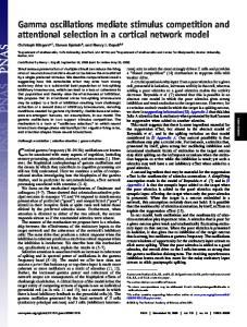
gamma peak. Bipolar differences were extracted from ECoG sensors covering a large part of the primate brain. Our goal in this study was to delineate the mechanisms underlying contrast specific effects. We tested these effects by allowing for trial-specific changes in model parameters. In particular, we considered a family of DCMs that allowed for contrast dependent changes in the strength of recurrent connections, the strength of intrinsic connections or the extent of intrinsic connections (or combinations thereof) and asked which model can best explain spectral responses for different contrast conditions, see Figure 4. The ability of each model to explain induced responses was evaluated in terms of their Bayesian model evidence; which provides a principled way to evaluate competing or complementary models or hypotheses.

Figure 4. Results of Bayesian Model Comparison. The model involving modulations of all parameters (model 7) has the highest evidence with a relative log evidence of 17 with respect to the model that allows for modulations in all but the extent parameters (model 6). The first three models correspond to hypotheses (i), (ii) and (iii) while models 4 and 5 to combinations (i) + (ii) and (ii) + (iii). The right panel shows the corresponding model posterior probabilities. These results suggest that we can be almost certain that all three synaptic mechanisms contribute to the formation of cross spectral data features. The first set of parameters comprised the gains of neural populations that are thought to encode precision errors. These gain parameters correspond to the precision (inverse variance or reliability) of prediction errors in predictive coding. This fits comfortably with neurobiological theories of attention under predictive coding and the hypothesis that contrast manipulation amounts to changes in the precision of sensory input, as reviewed in [65]. These changes affect hierarchical processing in the brain and control the interaction between bottom up sensory information and top down modulation: here, we focus on the sensory level of the visual hierarchy. The second set of parameters comprised intrinsic connection strengths among pyramidal and AIMS Neuroscience


32

spiny stellate cells and inhibitory interneurons. This speaks to variations in cortical excitability, which modulates the contributions of different neuronal populations under varying contrast conditions—and a fixed dispersion of lateral connections. This hypothesis fits comfortably well with studies focusing on the activation of reciprocally connected networks of excitatory and inhibitory neurons, including PING/ ING models [66–68]. The last set included the spatial extent of excitatory and inhibitory connections. From single cell recordings, it is known that as the boundary between classical and non-classical receptive field depends crucially upon contrast [26]. As stimulus contrast is decreased, the excitatory region becomes larger and the inhibitory flanks become smaller. The hypothesis here rests on a modulation of the effective spatial extent of lateral connections; effective extent refers to the extent of neuronal populations that subserve stimulus integration—that are differentially engaged depending on stimulus properties (as opposed to the anatomical extent of connections). Model comparison uses the evidence for models in data from all conditions simultaneously. The models we compared allowed only a subset of parameters to vary with contrast level, where each model corresponds to a hypothesis about contrast-specific effects on cortical responses. Specifically, (the log of) contrast dependent parameters were allowed to change linearly with the contrast level, such that the effect of contrast was parameterized by the sensitivity of contrast dependent parameters to contrast level. In summary, we considered three putative mechanisms of gain control that speak to models with and without contrast dependent effects on: (i) recurrent connections of neuronal populations, (ii) horizontal connections between excitatory and inhibitory pools of neurons and (iii) spatial dispersion of horizontal connections. These three model factors lead to 8 candidate models (or seven models excluding a model with no contrast dependent effects). Figure 4, shows three of the models that we considered. The seven (non-null) candidate models include the models depicted in Figure 4 and their combinations. The model with contrast dependent effects on all parameters (model 7) had the highest evidence with a relative log evidence difference of 17 with respect to the model that allows for modulations of all but the extent parameters (model 6). In these plots, the first three models correspond to hypotheses (i), (ii) and (iii) while models 4 and 5 to combinations (i) and (iii) and (ii) and (iii). In the right panel, we see the corresponding model posterior probabilities (assuming uniform priors over all models considered). This suggests that we can be almost certain that all three synaptic mechanisms contribute to the formation of cross spectral density features observed under different levels of visual contrast (given the models evaluated). Note that Figure 4 shows the relative log-evidence for each model normalised with respect to the lowest evidence; in this instance, the evidence of model (iii). A relative log evidence of three is usually taken to indicate a winning model. This corresponds to a likelihood ratio (log Bayes factor) of approximately 20:1. This is based on a free energy bound to model-evidence; this quantity can be written as the difference of a term quantifying accuracy minus a term quantifying complexity (see e.g. [46]). This characterization of model evidence results therefore in a winning model which is both accurate and parsimonious. Having identified the best model, we then examined its parameter estimates: the maximum a posteriori estimates are shown in Figure 5 (top), while estimates of their contrast sensitivity are shown in the lower panel. These results suggest that the largest contrast modulations are observed in (log scale parameter) estimates of connections to and from the superficial pyramidal cells. In particular, the largest variation over contrast is observed for the parameter that corresponds to the gain associated with superficial pyramidal cells. Here, an increase in contrast reduces the inhibitory self connection leading to a disinhibitory increase in gain. This result is in accord with the predictive AIMS Neuroscience


33

coding formulation above, where the gain of superficial pyramidal cells is thought to encode the precision of prediction errors. As contrast increases, confidence in (precision of) sensory information rises. In predictive coding this is thought to be accompanied by an increase in the weighting of sensory prediction errors that are generally thought to be reported by superficial pyramidal cells.

Figure 5. Parameter estimates and their changes. (A panel) Maximum a posteriori estimates of model parameters obtained after inverting model (vii). Note that these parameters represent the complete set of free parameters that are used to explain observed responses. (B) Corresponding sensitivity estimates of contrast dependent parameters. The largest contrast modulations are observed in estimates of connections to and from the superficial pyramidal cells (encircled). The contrast dependent changes in the extent of horizontal connectivity suggest an effective shrinking of excitatory horizontal influences and an increase in inhibitory effects. This is precisely what would be expected on the basis of contrast dependent changes in receptive field size. As contrast increases, receptive field sizes shrink—effectively passing higher frequency information to higher levels. In other words, the neural field has a more compact spatial summation that depends upon gain control and the balance of horizontal excitatory and inhibitory connections. For more details, we refer the reader to [10]. AIMS Neuroscience


34

4.

Conclusion

In this paper, we have considered neural field models in the light of a Bayesian framework for evaluating model evidence and obtaining parameter estimates using invasive and non-invasive recordings of gamma oscillations. We first focused on model predictions of conductance and convolution based field models and showed that these can yield spectral responses that are sensitive to biophysical properties of local cortical circuits like cortical excitability and synaptic filtering; we also considered two different mechanisms for this filtering: a nonlinear mechanism involving specific conductances and a linear convolution of afferent firing rates producing post synaptic potentials. We then turned to empirical MEG data and looked for potential determinants of the spectral properties of an individual's gamma response, and how they relate to underlying visual cortex microcircuitry and excitation/inhibition balance. We found correlations between peak gamma frequency and cortical inhibition (parameterized by the excitatory drive to inhibitory cell populations) over subjects. This constitutes a compelling illustration of how non-invasive data can provide quantitative estimates of the spatial properties of neural sources and explain systematic variations in the dynamics those sources generate. Furthermore, the conclusions fitted comfortably with studies of contextual interactions and orientation discrimination suggesting that local contextual interactions in V1 are weaker in individuals with a large V1 area [69,70]. Finally we used dynamic causal modeling and neural fields to test specific hypotheses about precision and gain control based on predictive coding formulations of neuronal processing. We exploited finely sampled electrophysiological responses from awake-behaving monkeys and an experimental manipulation (the contrast of visual stimuli) to look at changes in the gain and balance of excitatory and inhibitory influences. Our results suggest that increasing contrast effectively increases the sensitivity or gain of superficial pyramidal cells to inputs from spiny stellate populations. Furthermore, they are consistent with intriguing results showing that the receptive fields of V1 units shrinks with increasing visual contrast. The approach we have illustrated in this paper rests on neural field models that are optimized in relation to observed gamma responses from the visual cortex and are – crucially – compared in terms of their evidence. This provides a principled way to address questions about cortical structure, function and the architectures that underlie neuronal computations. Acknowledgments The Wellcome Trust funded this work. Conflict of Interest All authors declare no conflicts of interest in this paper. References 1. Pinotsis DA, Friston KJ. (2014). Neural fields, neural masses and Bayesian modelling. In Neural Fields: Theory and Applications. S. Coombes, P. beimGraben, R. Potthast, J. Wright (Eds.). Berlin: Springer-Verlag. 2. Deco G, Jirsa VK, Robinson PA, Breakspear M, Friston K. (2008) The Dynamic Brain: From AIMS Neuroscience


35

Spiking Neurons to Neural Masses and Cortical Fields. PLoS Comput Biol 4(8): e1000092. doi:10.1371/journal.pcbi.1000092. 3. Jirsa VK. (2004). Connectivity and dynamics of neural information processing. Neuroinformatics 2: 183-204. 4. Coombes S, Venkov NA, Shiau L, Bojak I, Liley DTJ, Laing CR. (2007) Modeling electrocortical activity through improved local approximations of integral neural field equations. Phys Rev E 76(5 Pt 1): 051901. 5. Robinson PA, Loxley PN, O’Connor SC, Rennie CJ. (2001) Modal analysis of corticothalamic dynamics, electroencephalographic spectra, and evoked potentials. Phys Rev E 63(4 Pt 1): 041909. 6. Breakspear M, Roberts JA, Terry JR, Rodrigues S, Mahant N, Robinson PA. (2006) A unifying explanation of primary generalized seizures through nonlinear brain modeling and bifurcation analysis. Cereb Cortex 16: 1296-1313. 7. Rodrigues S, Barton D, Szalai R, Benjamin O, Richardson MP, Terry JR. (2009) Transitions to spike-wave oscillations and epileptic dynamics in a human cortico-thalamic mean-field model. J comput neurosci 27: 507-526. 8. Pinotsis DA, Hansen E, Friston KJ, Jirsa VK. (2013) Anatomical connectivity and the resting state activity of large cortical networks. NeuroImage 65: 127-138. 9. Pinotsis DA, Schwarzkopf DS, Litvak V, Rees G, Barnes G, Friston KJ. (2013) Dynamic causal modelling of lateral interactions in the visual cortex. NeuroImage 66: 563-576. 10. Pinotsis DA, Brunet N, Bastos A, Bosman CA, Litvak V, Fries P, Friston KJ. (2014) Contrast gain-control and horizontal interactions in V1: A DCM study. NeuroImage 92C: 143-155 11. Riera JJ, Jimenez JC, Wan X, Kawashima R, Ozaki T. (2007) Nonlinear local electrovascular coupling. II: From data to neuronal masses. Hum brain mapp 28: 335-354. 12. Schiff S, Sauer T. (2008) Kalman filter control of a model of spatiotemporal cortical dynamics. BMC Neurosci 5(1): 1-8. 13. Angelucci A, Bressloff PC. (2006) Contribution of feedforward, lateral and feedback connections to the classical receptive field center and extra-classical receptive field surround of primate V1 Neurons. Prog Brain Res 154: 93-120. 14. Burkhalter A, Bernardo KL. (1989) Organization of corticocortical connections in human visual cortex. Proc Natl Acad Sci USA 86(3): 1071-5. 15. Wallace MN, Bajwa S. ( 1991) Patchy intrinsic connections of the ferret primary auditory cortex. Neuroreport 2(8): 417-20. 16. Stettler DD, Das A, Bennett J, Gilbert CD. (2002) Lateral connectivity and contextual interactions in macaque primary visual cortex. Neuron 36: 739-750. 17. Baker TI, Cowan JD. (2009) Spontaneous pattern formation and pinning in the primary visual cortex. J Physio Paris 103: 52-68. 18. Wen Q, Chklovskii DB. (2008) A cost–benefit analysis of neuronal morphology. J neurophysiol 99: 2320-2328. 19. Cherniak C. (1994) Component placement optimization in the brain. J neurosci 14: 2418-2427. 20. Bassett DS, Greenfield DL, Meyer-Lindenberg A, Weinberger DR, Moore SW, Bullmore ET. (2010) Efficient physical embedding of topologically complex information processing networks in brains and computer circuits. PLoS comput biol 6(4): e1000748. doi:10.1371/journal.pcbi.1000748 21. Grindrod P, Pinotsis DA. (2011) On the spectra of certain integro-differential-delay problems with applications in neurodynamics. Physica D 240: 13-20. AIMS Neuroscience


36

22. Pinotsis DA, Friston KJ. (2011) Neural fields, spectral responses and lateral connections. Neuroimage 55: 39-48. 23. Sceniak MP, Hawken MJ, Shapley R. (2001). Visual spatial characterization of macaque V1 neurons. J Neurophysiol 85: 1873-1887. 24. Sceniak MP, Chatterjee S, Callaway EM. (2006) Visual spatial summation in macaque geniculocortical afferents. J Neurophysiol 96: 3474-3484. 25. Sceniak MP, Ringach DL, Hawken MJ, Shapley R. (1999) Contrast’s effect on spatial summation by macaque V1 neurons. Nat neurosci 2: 733-739. 26. Kapadia MK, Westheimer G, Gilbert CD. (1999) Dynamics of spatial summation in primary visual cortex of alert monkeys. Proc Natl Acad Sci USA 96: 12073-12078. 27. Ray S, Maunsell JH. (2010) Differences in gamma frequencies across visual cortex restrict their possible use in computation. Neuron 67(5): 885-896. 28. Hodgkin AL, Huxley AF. (1952) A quantitative description of membrane current and its application to conduction and excitation in nerve. J physiol 117(4): 500-544. 29. Traub RD, Kopell N, Bibbig A, Buhl EH, LeBeau FE, Whittington MA. (2001) Gap junctions between interneuron dendrites can enhance synchrony of gamma oscillations in distributed networks. J Neurosci 21: 9478-9486. 30. Moran RJ, Stephan KE, Kiebel SJ, Rombach N, O’Connor WT, Murphy KJ, Reilly RB, Friston KJ. (2008) Bayesian estimation of synaptic physiology from the spectral responses of neural masses. Neuroimage 42: 272-84. 31. Moran RJ, Stephan KE, Dolan RJ, Friston KJ. (2011) Consistent spectral predictors for dynamic causal models of steady-state responses. Neuroimage 55: 1694-1708. 32. Goldstein SS, Rall W. (1974) Changes of action potential shape and velocity for changing core conductor geometry. Biophys J 14: 731-757. 33. Ellias SA, Grossberg S. (1975) Pattern formation, contrast control, and oscillations in the short term memory of shunting on-center off-surround networks. Biol Cybern 20: 69-98. 34. Somers DC, Nelson SB, Sur M. (1995) An emergent model of orientation selectivity in cat visual cortical simple cells. J neurosci 15: 5448-5465. 35. Ermentrout B. (1998) Neural networks as spatio-temporal pattern-forming systems. Rep progin phys 61: 353. 36. Jansen BH, Rit VG. (1995) Electroencephalogram and visual evoked potential generation in a mathematical model of coupled cortical columns. Biol Cybern 73: 357-66. 37. Pinotsis D, Leite M, Friston K. (2013) On conductance-based neural field models. Front. Comput. Neurosci 7: 158. doi: 10.3389/fncom.2013.00158. 38. Pinotsis DA, Moran RJ, Friston KJ. (2012) Dynamic causal modeling with neural fields. Neuroimage 59: 1261-1274. 39. Faulkner HJ, Traub RD, Whittington MA. (2009) Disruption of synchronous gamma oscillations in the rat hippocampal slice: A common mechanism of anaesthetic drug action. Brit pharmacol 125: 483-492. 40. Moran RJ, Jung F, Kumagai T, Endepols H, Graf R, Dolan RJ, Friston KJ, Stephan KE, Tittgemeyer M. (2011) Dynamic causal models and physiological inference: a validation study using isoflurane anaesthesia in rodents. PloS one 6: e22790. 41. Pinotsis DA, Moran RJ, Friston KJ. (2012) Dynamic causal modeling with neural fields. NeuroImage 59: 1261-1274. 42. Bastos AM, Usrey WM, Adams RA, Mangun GR, Fries P, Friston KJ. (2012) Canonical microcircuits for predictive coding. Neuron 76: 695-711. AIMS Neuroscience


37

43. Buffalo EA, Fries P, Landman R, Buschman TJ, Desimone R. (2011) Laminar differences in gamma and alpha coherence in the ventral stream. Proc Natl Acad Sci USA 108: 11262. 44. Haider B, Duque A, Hasenstaub AR, McCormick DA. (2006) Neocortical network activity in vivo is generated through a dynamic balance of excitation and inhibition. J neurosci 26: 4535-4545. 45. Jansen BH, Rit VG. (1995) Electroencephalogram and visual evoked potential generation in a mathematical model of coupled cortical columns. Biol Cybern 73:357-66. 46. Friston K, Mattout J, Trujillo-Barreto N, Ashburner J, Penny W. (2007). Variational free energy and the Laplace approximation. Neuroimage 34: 220-234. 47. Wilson HR, Cowan JD. (1973) Mathematical Theory of Functional Dynamics of Cortical and Thalamic Nervous-Tissue. Kybernetik 13: 55-80. 48. Pelinovsky DE, Yakhno VG. (1996) Generation of collective-activity structures in a homogeneous neuron-like medium. I. Bifurcation analysis of static structures. Int J Bifurcat Chaos 6: 81-88. 49. Pinto DJ, Brumberg JC, Simons DJ, Ermentrout GB. (1996) A quantitative population model of whisker barrels: re-examining the Wilson-Cowan equations. J Comput Neurosci 3: 247-64. 50. Robinson PA, Rennie CJ, Rowe DL, O’Connor SC, Gordon E. (2005) Multiscale brain modelling. Philos T Roy Soc B 360: 1043-1050. 51. Coombes S. (2005) Waves, bumps, and patterns in neural field theories. Biol Cybern 93: 91-108. 52. Valdes PA, Jimenez JC, Riera J, Biscay R, Ozaki T. (1999) Nonlinear EEG analysis based on a neural mass model. Biol cybern 81: 415-424. 53. Robinson PA, Loxley PN, O’Connor SC, Rennie CJ. (2001) Modal analysis of corticothalamic dynamics, electroencephalographic spectra, and evoked potentials. Phys Rev E 63(4 Pt 1): 041909 54. Kopell N, Ermentrout GB, Whittington MA, Traub RD. (2000) Gamma rhythms and beta rhythms have different synchronization properties. Proc Natl Acad Sci USA 97: 1867-72. 55. Jia X, Xing D, Kohn A. (2013) No consistent relationship between gamma power and peak frequency in macaque primary visual cortex. J Neurosci 33: 17-25. 56. Chambers JD, Bethwaite B, Diamond NT, Peachey T, Abramson D, Petrou S, Thomas EA. (2012) Parametric computation predicts a multiplicative interaction between synaptic strength parameters that control gamma oscillations. Front Comput Neurosci 6:53 doi: 10.3389/fncom.2012.00053. 57. Schwarzkopf DS, Robertson DJ, Song C, Barnes GR, Rees G. (2012) The Frequency of Visually Induced Gamma-Band Oscillations Depends on the Size of Early Human Visual Cortex. J Neurosci 32: 1507-1512. 58. Schwarzkopf DS, Robertson DJ, Song C, Barnes GR, Rees G. (2012) The Frequency of Visually Induced Gamma-Band Oscillations Depends on the Size of Early Human Visual Cortex. J Neurosci 32: 1507-1512. 59. Muthukumaraswamy SD, Edden RA., Jones DK, Swettenham JB, Singh KD. (2009) Resting GABA concentration predicts peak gamma frequency and fMRI amplitude in response to visual stimulation in humans. Proc Natl Acad Sci 106: 8356-8361. 60. Pinotsis DA, Friston KJ. (2011) Neural fields, spectral responses and lateral connections. Neuroimage 55: 39-48. 61. Gaetz W, Roberts TP., Singh KD, Muthukumaraswamy SD. (2011) Functional and structural correlates of the aging brain: Relating visual cortex (V1) gamma band responses to age‐related structural change. Hum Brain Mapp 33(9): 2035-46. AIMS Neuroscience


38

62. Muthukumaraswamy SD, Edden RA., Jones DK, Swettenham JB, Singh KD. (2009) Resting GABA concentration predicts peak gamma frequency and fMRI amplitude in response to visual stimulation in humans. Proc Natl Acad Sci 106: 8356-8361. 63. Rubehn B, Bosman C, Oostenveld R, Fries P, Stieglitz T: A MEMS-based flexible multichannel ECoG-electrode array. J. Neural Eng 6 036003 doi:10.1088/1741-2560/6/3/036003. 64. Bosman CA, Schoffelen J-M, Brunet N, Oostenveld R, Bastos AM, Womelsdorf T, Rubehn B, Stieglitz T, De Weerd P, Fries P. (2009) Attentional stimulus selection through selective synchronization between monkey visual areas. Neuron 75: 875-888. 65. Feldman H, Friston KJ. (2010) Attention, uncertainty, and free-energy. Front Hum Neurosci 4: 215. doi: 10.3389/fnhum.2010.00215. 66. Kang K, Shelley M, Henrie JA, Shapley R. (2010) LFP spectral peaks in V1 cortex: network resonance and cortico-cortical feedback. J computat neurosci 29: 495-507. 67. Brunel N, Wang X-J. (2003) What determines the frequency of fast network oscillations with irregular neural discharges? I. Synaptic dynamics and excitation-inhibition balance. J Neurophysiol 90: 415-430. 68. Traub RD, Jefferys JG, Whittington MA. (1997) Simulation of gamma rhythms in networks of interneurons and pyramidal cells. J comput neurosci 4: 141-150. 69. Schwarzkopf DS, Song C, Rees G. (2011) Linking perceptual experience with the functional architecture of the visual cortex. J Vis 11: 844-844. 70. Harvey BM, Dumoulin SO. (2011) The Relationship between Cortical Magnification Factor and Population Receptive Field Size in Human Visual Cortex: Constancies in Cortical Architecture. J Neurosci 31: 13604-13612. @2014, Dimitris Pinotsis et al., licensee AIMS Press. This is an open access article distributed under the terms of the Creative Commons Attribution License (http://creativecommons.org/licenses/by/4.0)

AIMS Neuroscience
