Gasoline: An adaptable implementation of TreeSPH
arXiv:astro-ph/0303521v1 24 Mar 2003
J.W. Wadsley a J. Stadel b T. Quinn c a Department b Institute c Astronomy
of Physics and Astronomy, McMaster University, Hamilton, Canada 1 for Theoretical Physics, University of Zurich, Switzerland
Department, University of Washington, Seattle, Washington, USA
Abstract The key algorithms and features of the Gasoline code for parallel hydrodynamics with self-gravity are described. Gasoline is an extension of the efficient Pkdgrav parallel N -body code using smoothed particle hydrodynamics. Accuracy measurements, performance analysis and tests of the code are presented. Recent successful Gasoline applications are summarized. These cover a diverse set of areas in astrophysics including galaxy clusters, galaxy formation and gas-giant planets. Future directions for gasdynamical simulations in astrophysics and code development strategies for tackling cutting edge problems are discussed. Key words: Hydrodynamics, Methods: numerical, Methods: N-body simulations, Dark matter PACS: 02.60.Cb, 95.30.Lz, 95.35.+d
1
Introduction
Astrophysicists have always been keen to exploit technology to better understand the universe. N-body simulations predate the use of digital computers with the use of light bulbs and light intensity measurements as an analog of gravity for manual simulations of a many-body self-gravitating system (Holmberg 1947). Astrophysical objects including planets, individual stars, interstellar clouds, star clusters, galaxies, accretion disks, clusters of galaxies 1
E-mail:
[email protected]
Preprint submitted to Elsevier Science
2 February 2008
through to large scale structure have all the been the subject of numerical investigations. The most challenging extreme is probably the evolution of spacetime itself in computational general relativistic simulations of colliding neutron stars and black holes. Since the advent of digital computers, improvements in storage and processing power have dramatically increased the scale of achievable simulations. This, in turn, has driven remarkable progress in algorithm development. Increasing problem sizes have forced simulators who were once content with O(N 2 ) algorithms to pursue more complex O(N log N) and, with limitations, even O(N) algorithms and adaptivity in space and time. In this context we present Gasoline, a parallel N-body and gasdynamics code, which has enabled new light to be shed on a range of complex astrophysical systems. The discussion is presented in the context of future directions in numerical simulations in astrophysics, including fundamental limitations in serial and parallel.
We begin by tracing past progress in computational astrophysics with an initial focus on self-gravitating systems (N-body dynamics) in section 2. Gasoline evolved from the Pkdgrav parallel N-body tree code designed by (Stadel 2001). The initial modular design of Pkdgrav and a collaborative programming model using CVS for source code management has facilitated several simultaneous developments from the Pkdgrav code base. These include inelastic collisions (e.g. planetesimal dynamics, Richardson et al. 2000), gas dynamics (Gasoline) and star formation. In section 3 we summarize the essential gravity code design, including the parallel data structures and the details of the tree code as applied to calculating gravitational forces. We complete the section with a brief examination of the gravitational force accuracy.
In section 4 we examine aspects of hydrodynamics in astrophysical systems to motivate Smoothed Particle Hydrodynamics (SPH) as our choice of fluid dynamics method. We describe the Gasoline SPH implementation in section 5, including neighbour finding algorithms and the cooling implementation.
Interesting astrophysical systems usually exhibit a large range of time scales. Tree codes are very adaptable in space; however, time-adaptivity has become important for leading edge numerical simulations. In section 6 we describe our hierarchical timestepping scheme. Following on in section 7 we examine the performance of Gasoline when applied to challenging numerical simulations of real astrophysical systems. In particular, we examine the current and potential benefits of multiple timesteps for time adaptivity in areas such as galaxy and planet formation. We present astrophysically oriented tests used to validate Gasoline in section 8. We conclude by summarizing current and proposed applications for Gasoline. 2
2
Gravity
Gravity is the key driving force in most astrophysical systems. With assumptions of axisymmetry or perturbative approaches an impressive amount of progress has been made with analytical methods, particularly in the areas of solar system dynamics, stability of disks, stellar dynamics and quasi-linear aspects of the growth of large scale structure in the universe. In many systems of interest, however, non-linear interactions play a vital role. This ultimately requires the use of self-gravitating N-body simulations. Fundamentally, solving gravity means solving Poisson’s equation for the gravitational potential, φ, given a mass density, ρ: ∇2 φ = 4πGρ where G is the Newtonian gravitational constant. In a simulations with discrete bodies it is common to start from the explicit expression for the acceleration, ai = ∇φ on a given body in terms of the sum of the influence of all other bodies, P ai = i6=j GMj /(ri − rj )2 where the ri and Mi are the position and masses of the bodies respectively. When attempting to model collisionless systems, these same equations are the characteristics of the collisionless Boltzmann equation, and the bodies can be thought of as samples of the distribution function. In practical work it is essential to soften the gravitational force on some scale r < ǫ to avoid problems with the integration and to minimize two-body scattering in cases where the bodies represent a collisionless system. Early N-body work such as studies of relatively small stellar systems were approached using a direct summation of the forces on each body due to every other body in the system (Aarseth 1975). This direct O(N 2 ) approach is impractical for large numbers of bodies, N, but has enjoyed a revival due to incredible throughput of special purpose hardware such as GRAPE (Hut & Makino 1999). The GRAPE hardware performs the mutual force calculation for sets of bodies entirely in hardware and remains competitive with other methods on more standard floating hardware up to N ∼ 100, 000. A popular scheme for larger N is the Particle-Mesh (PM) method which has long been used in electrostatics and plasma physics. The adoption of PM was strongly related to the realization of the existence of the O(N log N) Fast Fourier Transform (FFT) in the 1960’s. The FFT is used to solve for the gravitational potential from the density distribution interpolated onto a regular mesh. In astrophysics sub-mesh resolution is often desired, in which case the force can be corrected on sub-mesh scales with local direct sums as in the Particle-Particle Particle-Mesh (P3 M) method. PM is popular in stellar disk dynamics, and P3 M has seen widespread adoption in cosmology (e.g. Efstathiou et al. 1985). PM codes have similarities with multigrid (e.g. Press et al. 1995) and other iterative schemes. However, working in Fourier space is not only more efficient, but it also allows efficient force error control through opti3
mization of the Green’s function and smoothing. Fourier methods are widely recognised as ideal for large, fairly homogeneous, periodic gravitating simulations. Multigrid has some advantages in parallel due to the local nature of the iterations. The Particle-Particle correction can get expensive when particles cluster in a few cells. Both multigrid (e.g. Fryxell et al. 2000, Kravtsov et al. 1997) and P3 M (AP3 M: Couchman 1991) can adapt to address this via a hierarchy of sub-meshes. With this approach the serial slow down due to heavy clustering tends toward a fixed multiple of the unclustered run speed. In applications such as galactic dynamics where high resolution in phase space is desirable and particle noise is problematic, the smoothed gravitational potentials provided by an expansion in modes is useful. PM does this with Fourier modes; however, a more elegant approach is the Self-Consistent Field method (SCF) (Hernquist & Ostriker 1992, Weinberg 1999). Using a basis set closely matched to the evolving system dramatically reduces the number of modes to be modelled; however, the system must remain close to axi-symmetric and similar to the basis. SCF parallelizes well and is also used to generate initial conditions such as stable individual galaxies that might be used for merger simulations. A current popular choice is to use tree algorithms which are inherently O(N log N). This approach recognises that details of the remote mass distribution become less important for accurate gravity with increasing distance. Thus the remote mass distribution can be expanded in multipoles on the different size scales set by a tree-node hierarchy. The appropriate scale to use is set by the opening angle subtended by the tree-node bounds relative to the point where the force is being calculated. The original Barnes-Hut (Barnes & Hut 1986) method employed oct-trees but this is not especially advantageous, and other trees also work well (Jernighan & Porter 1989). The tree approach can adapt to any topology, and thus the speed of the method is somewhat insensitive to the degree of clustering. Once a tree is built it can also be re-used as an efficient search method for other physics such as particle based hydrodynamics. A particularly useful property of tree codes is the ability to efficiently calculate forces for a subset of the bodies. This is critical if there is a large range of timescales in a simulation and multiple independent timesteps are employed. At the cost of force calculations no longer being synchronized among the particles substantial gains in time-to-solution may be realized. Multiple timesteps are particularly important for current astrophysical applications where the interest and thus resolution tends to be focused on small regions within large simulated environments such as individual galaxies, stars or planets. Dynamical times can become very short for small numbers of particles. P3 M codes are faster for full force calculations but are difficult to adapt to calculate a subset of the forces. 4
In order to treat periodic boundaries with tree codes it is necessary to effectively infinitely replicate the simulation volume which may be approximated with an Ewald summation (Hernquist, Bouchet & Suto 1991). An efficient alternative which is seeing increasing use is to use trees in place of the direct Particle-Particle correction to a Particle-Mesh code, often called Tree-PM (Wadsley 1998, Bode, Ostriker & Xu 2000, Bagla 2002). The Fast Multipole Method (FMM) recognises that the applied force as well as the mass distribution may be expanded in multipoles. This leads to a force calculation step that is O(N) as each tree node interacts with a similar number of nodes independent of N and the number of nodes is proportional to the number of bodies. Building the tree is still O(N log N) but this is a small cost for simulations up to N ∼ 107 (Dehnen 2000). The Greengard & Rokhlin (1987) method used spherical harmonic expansions where the desired accuracy is achieved solely by changing the order of the expansions. For the majority of astrophysical applications the allowable force accuracies make it much more efficient to use fixed order Cartesian expansions and an opening angle criterion similar to standard tree codes (Salmon & Warren 1994, Dehnen 2000). This approach has the nice property of explicitly conserving momentum (as do PM and P3 M codes). The prefactor for Cartesian FMM is quite small so that it can outperform tree codes even for small N (Dehnen 2000). It is a significantly more complex algorithm to implement, particularly in parallel. One reason widespread adoption has not occurred is that the speed benefit over a tree code is significantly reduced when small subsets of the particles are having forces calculated (e.g. for multiple timesteps).
3
Solving Gravity in Gasoline
Gasoline is built on the Pkdgrav framework and thus uses the same gravity algorithms. The Pkdgrav parallel N-body code was designed by Stadel and developed in conjunction with Quinn beginning in the early 90’s. This includes the parallel code structure and core algorithms such as the tree structure, tree walk, hexadecapole multipole calculations for the forces and the Ewald summation. There have been additional contributions to the gravity code by Richardson and Wadsley in the form of minor algorithmic modifications and optimizations. The latter two authors became involved as part of the collisions and Gasoline extensions of the original Pkdgrav code respectively. We have summarized the gravity method used in the production version of Gasoline without getting into great mathematical detail. For full technical details on Pkdgrav the reader is referred to Stadel (2001). 5
3.1 Design Gasoline is fundamentally a tree code. It uses a variant on the K-D tree (see below) for the purpose of calculating gravity, dividing work in parallel and searching. Stadel (2001) designed Pkdgrav from the start as a parallel code. There are four layers in the code. The Master layer is essentially serial code that orchestrates overall progress of the simulation. The Processor Set Tree (PST) layer distributes work and collects feedback on parallel operations in an architecture independent way using MDL. The Machine Dependent Layer (MDL) is a relatively short section of code that implements remote procedure calls, effective memory sharing and parallel diagnostics. All processors other than the master loop in the PST level waiting for directions from the single process executing the Master level. Directions are passed down the PST in a tree based O(log2 NP ) procedure that ends with access to the fundamental bulk particle data on every node at the PKD level. The Parallel K-D (PKD) layer is almost entirely serial but for a few calls to MDL to access remote data. The PKD layer manages local trees for gravity and particle data and is where the physics is implemented. This modular design enables new physics to be coded at the PKD level without requiring detailed knowledge of the parallel framework. 3.2 Mass Moments Pkdgrav departed significantly from the original N-body tree code designs of Barnes & Hut (1986) by using 4th (hexadecapole) rather than 2nd (quadrupole) order multipole moments to represent the mass distribution in cells at each level of the tree. This results in less computation for the same level of accuracy: better pipelining, smaller interaction lists for each particle and reduced communication demands in parallel. The current implementation in Gasoline uses reduced moments that require only n + 1 terms to be stored for the nth moment. For a detailed discussion of the accuracy and efficiency of the tree algorithm as a function the order of the multipoles used see (Stadel 2001) and (Salmon & Warren 1994). 3.3 The Tree The original K-D tree (Bentley 1979) was a balanced binary tree. Gasoline divides the simulation in a similar way using recursive partitioning. At the PST level this is parallel domain decomposition and the division occurs on the longest axis to recursively divide the work among the remaining processors. Even divisions occur only when an even number of processors remains. 6
Otherwise the work is split in proportion to the number of processors on each side of the division. Thus, Gasoline may use arbitrary numbers of processors and is efficient for flat topologies without adjustment. At the PST level each processor has a local rectangular domain within which a local binary tree is built. The structure of the lower tree is important for the accuracy of gravity and efficiency of other search operations such as neighbour finding required for SPH. Oct-trees (e.g. Barnes & Hut 1986, Salmon & Warren 1994) are traditional in gravity codes. In contrast, the key data structures used by Gasoline are spatial binary trees. One immediate gain is that the local trees do not have to respect a global structure and simply continue from the PST level domain decomposition in parallel. The binary tree determines the hierarchical representation of the mass distribution with multipole expansions, of which the root node or cell encloses the entire simulation volume. The local gravity tree is built by recursively bisecting the longest axis of each cell which keeps the cells axis ratios close to one. In contrast, cells in standard K-D trees can have large axis ratios which lead to large multipoles and with correspondingly large gravity errors. At each level the dimensions of the cells are squeezed to just contain the particles. This overcomes the empty cell problem of un-squeezed spatial bisection trees. The SPH tree is currently a balanced K-D tree; however, testing indicates that the efficiency gain is slight and it is not worth the cost of an additional tree build. The top down tree build process is halted when nBucket or fewer particles remain in a cell. Stopping the tree with nBucket particles in a leaf cell reduces the storage required for the tree and makes both gravity and search operations more efficient. For these purposes nBucket ∼ 8 − 16 is a good choice. Once the gravity tree has been built there is a bottom-up pass starting from the buckets and proceeding to the root, calculating the center of mass and the multipole moments of each cell from the center of mass and moments of each of its two sub-cells.
3.4 The Gravity Walk
Gasoline calculates the gravitational accelerations using the well known treewalking procedure of the Barnes & Hut (1986) algorithm, except that it collects interactions for entire buckets rather than single particles. This amortizes the cost of tree traversal for a bucket over all its particles. In the tree building phase, Gasoline assigns to each cell of the tree an opening 7
Bucket Cell Bmax
ropen
B1
B2
CM
Fig. 1. Opening radius for a cell in the tree, intersecting bucket B1 and not bucket B2 . This cell is “opened” when walking the tree for B1 . When walking the tree for B2 , the cell will be added to the particle-cell interaction list of B2 .
radius about its center-of-mass. This is defined as, 2Bmax ropen = √ 3θ
(1)
where Bmax is the maximum distance from a particle in the cell to the centerof-mass of the cell. The opening angle, θ, is a user specified accuracy parameter which is similar to the traditional θ parameter of the Barnes-Hut code; notice that decreasing θ in equation 1, increases ropen . The opening radii are used in the Walk phase of the algorithm as follows: for each bucket Bi , Gasoline starts descending the tree, opening those cells whose ropen intersect with Bi (see Figure 1). If a cell is opened, then Gasoline repeats the intersection-test with Bi for the cell’s children Otherwise, the cell is added to the particle-cell interaction list of Bi . When Gasoline reaches the leaves of the tree and a bucket Bj is opened, all of Bj ’s particles are added to the particle-particle interaction list of Bi . Once the tree has been traversed in this manner we can calculate the gravitational acceleration for each particle of Bi by evaluating the interactions specified in the two lists. Gasoline uses the hexadecapole multipole expansion to calculate particle-cell interactions.
3.5 Softening The particle-particle interactions are softened to lessen two-body relaxation effects that compromise the attempt to model continuous fluids, including the collisionless dark matter fluid. In Gasoline the particle masses are effectively smoothed in space using the same spline form employed for SPH in section 5. 8
This means that the gravitational forces vanish at zero separation and return to Newtonian 1/r 2 at a separation of ǫi + ǫj where ǫi is the gravitational softening applied to each particle. In this sense the gravitational forces are well matched to the SPH forces. 3.6 Periodicity A disadvantage of tree codes is that they must deal explicitly with periodic boundary conditions (as are usually required for cosmology). Gasoline incorporates periodic boundaries via the Ewald summation technique where the force is divided into short and long range components. The Gasoline implementation differs from that of Hernquist, Bouchet & Suto (1991) in using a new technique due to Stadel (2001) based on an hexadecapole moment expansion of the fundamental cube to drastically reduce the work for the long range Ewald sum that approximates the infinite periodic replications. For each particle the computations are local and fixed, and thus the algorithm scales exceedingly well. There is still substantial additional work in periodic simulations because particles interact with cells and particles in nearby replicas of the fundamental cube (similar to Ding et al. 1992). 3.7 Force Accuracy The tree opening criteria places a bound on the relative error due to a single particle-cell interaction. As Gasoline uses hexadecapoles the error bound improves rapidly as the opening angle, θ, is lowered. The relationship between the typical (e.g. rms) relative force error and opening angle is not a straightforward power-law in θ because the net gravitational forces on each particle result from the cancellation of many opposing forces. In figure 2, we show a histogram of the relative acceleration errors for a cosmological Gasoline simulations at two different epochs for a range of opening angles. We have plotted the error curves as cumulative fractions to emphasize the limited tails to high error values. For typical gasoline simulations we commonly use θ = 0.7 which gives an rms relative error of 0.0039 for the clustered final state referred to by the left panel of figure 2. The errors relative to the mean acceleration (figure 3) are larger (rms 0.0083) but of less interest for highly clustered cases. As a simulated medium becomes more uniform the net gravitational accelerations approach zero. In a tree code the small forces result from the cancellation of large opposing forces. This is the case in cosmology at early times when the perturbations ultimately leading to cosmological structures are still small. In this situation it is essential to tighten the cell-opening criterion to increase the relative accuracy so that the net accelerations are sufficiently accurate. For 9
θ = 1.1
1.0000
θ = 1.1
1.0000
0.9
0.7
0.1000
Cumulative Fraction
Cumulative Fraction
0.9
0.5 0.3 0.0100 0.1
0.0010
0.5 0.4 0.0100 0.3 0.1 0.0010
z=0 0.0001 10-5
0.7
0.1000
10-4 10-3 10-2 10-1 Relative error, |δai|/|ai|
z=19 100
0.0001 10-5
10-4 10-3 10-2 10-1 Relative error, |δai|/|ai|
100
Fig. 2. Gasoline relative errors, for various opening angles θ. The distributions are all for a 323 , 64 Mpc box where the left panel represents the clustered final state and the right an initial condition (redshift z = 19). Typical values of θ = 0.5 and 0.7 are shown as thick lines. The solid curves compare to exact forces and thus have a minimum error set by the parameters of the Ewald summation whereas the dotted curves compare to the θ = 0.1 case. The Ewald summation errors only become noticeable for θ < 0.4. Relative errors are best for clustered objects but over-emphasize errors for low acceleration particles that are common in cosmological initial conditions.
example in the right hand panels of figures 2 and 3 the errors are larger, and at z = 19, the rms relative error is 0.041 for θ = 0.7. However, here the absolute errors are lower by nearly a factor of two in rms (0.026) as shown in figure 3. At early times when the medium fairly homogeneous growth is driven by local gradients, and thus acceleration errors normalized to the mean acceleration provide the better measure of accuracy as large relative errors are meaningless for accelerations close to zero. To ensure accurate integrations we switch to values such as θ = 0.5 before z = 2, giving an rms relative error of 0.0077 and an rms error of 0.0045 normalized to the mean absolute acceleration for the z = 19 distribution (a reasonable start time for a cosmological simulation on this scale).
4
Gasdynamics
Astrophysical systems are predominantly at very low physical densities and experience wide-ranging temperature variations. Most of the material is in a highly compressible gaseous phase. In general this means that a perfect adiabatic gas is an excellent approximation for the system. Microscopic physical processes such as shear viscosity and diffusion can usually be neglected. 10
θ = 1.1
1.0000
θ = 1.1
1.0000
0.9
0.7
0.1000
Cumulative Fraction
Cumulative Fraction
0.9
0.5 0.3 0.0100 0.1
0.0010
0.5 0.4 0.0100 0.3 0.1 0.0010
z=0 0.0001 10-5
0.7
0.1000
10-4 10-3 10-2 10-1 Error relative to mean, |δai|/
z=19 100
0.0001 10-5
10-4 10-3 10-2 10-1 Error relative to mean, |δai|/
100
Fig. 3. Gasoline errors relative to the mean for the same cases as Fig. 2. The errors are measured compared to the mean acceleration (magnitude) averaged over all the particles. Errors relative to the mean are more appropriate to judge accuracy for small accelerations resulting from force cancellation in a nearly homogeneous medium.
High-energy processes and the action of gravity tend to create large velocities so that flows are both turbulent and supersonic: strong shocks and very high Mach numbers are common. Radiative cooling processes can also be important; however, the timescales can often be much longer or shorter than dynamical timescales. In the latter case isothermal gas is often assumed for simplicity. In many areas of computational astrophysics, particularly cosmology, gravity tends to be the dominating force that drives the evolution of the system. Visible matter, usually in the form of radiating gas, provides the essential link to observations. Radiative transfer is always present but may not significantly affect the energy and thus pressure of the gas during the simulation. Fluid dynamics solvers can be broadly classified into Eulerian or Lagrangian methods. Eulerian methods use a fixed computational mesh through which the fluid flows via explicit advection terms. Regular meshes provide for ease of analysis and thus high order methods such as PPM (Woodward & Collela 1984) and TVD schemes (e.g. Harten et al. 1987, Kurganov & Tadmor 2000) have been developed. The inner loops of mesh methods can often be pipelined for high performance. Lagrangian methods follow the evolution of fluid parcels via the full (comoving) derivatives. This requires a deforming mesh or a meshless method such as Smoothed Particle Hydrodynamics (SPH) (Monaghan 1992). Data management is more complex in these methods; however, advection is handled implicitly and the simulation tends to naturally adapt to follow density contrasts. 11
Large variations in physical length scales in astrophysics have limited the usefulness of Eulerian grid codes. Adaptive Mesh Refinement (AMR) (Fryxell et al. 2000, Bryan & Norman 1997) overcomes this at the cost of data management overheads and increased code complexity. In the cosmological context there is the added complication of dark matter. There is more dark matter than gas in the universe so it dominates the gravitational potential. Perturbations present on all scales in the dark matter guide the formation of gaseous structures including galaxies and the first stars. A fundamental limit to AMR in computational cosmology is matching the AMR resolution to the underlying dark matter resolution. Particle based Lagrangian methods such as SPH are well matched to this constraint. A useful feature of Lagrangian simulations is that bulk flows (which can be highly supersonic in the simulation frame) do not limit the timesteps. Particle methods are well suited to rapidly rotating systems such as astrophysical disks where arbitrarily many rotation periods may have to be simulated (e.g. SPH explicitly conserves angular momentum). A key concern for all methods is correct angular momentum transport.
5
Smoothed Particle Hydrodynamics in Gasoline
Smoothed Particle Hydrodynamics is an approach to hydrodynamical modelling developed by Lucy (1977) and Gingold & Monaghan (1977). It is a particle method that does not refer to grids for the calculation of hydrodynamical quantities: all forces and fluid properties are found on moving particles eliminating numerically diffusive advective terms. The use of SPH for cosmological simulations required the development of variable smoothing to handle huge dynamic ranges (Hernquist & Katz 1989). SPH is a natural partner for particle based gravity. SPH has been combined with P3 M (Evrard 1988), Adaptive P3 M (HYDRA, Couchman et al. 1995), GRAPE (Steinmetz 1996) and tree gravity (Hernquist & Katz 1989). Parallel codes using SPH include Hydra MPI, Parallel TreeSPH (Dave, Dubinski & Hernquist 1997) and the GADGET tree code (Springel et al. 2001). The basis of the SPH method is the representation and evolution of smoothly varying fluid quantities whose value is only known at disordered discrete points in space occupied by particles. Particles are the fundamental resolution elements comparable to cells in a mesh. SPH functions through local summation operations over particles weighted with a smoothing kernel, W , that approximates a local integral. The smoothing operation provides a basis from which to obtain derivatives. Thus, estimates of density related physical quantities and gradients are generated. The summation aspect led to SPH being described √ as a Monte Carlo type method (with O(1/ N ) errors) however it was shown by Monaghan (1985) that the method is more closely related to interpolation theory with errors O((lnN)d /N), where d is the number of dimensions. 12
A general smoothed estimate for some quantity f at particle i given particles j at positions ~rj takes the form:
fi,smoothed =
n X
j=1
fj Wij (~ri − ~rj , hi , hj ),
(2)
where Wij is a kernel function and hj is a smoothing length indicative of the range of interaction of particle j. It is common to convert this particleweighted sum to volume weighting using fj mj /ρj in place of fj where the mj and ρj are the particle masses and densities, respectively. For momentum and energy conservation in the force terms, a symmetric Wij = Wji is required. We use the kernel-average first suggested by Hernquist & Katz (1989), 1 1 Wij = w(|~ri − ~rj |/hi ) + w(|~ri − ~rj |/hj ) 2 2
(3)
For w(x) we use the standard spline form with compact support where w = 0 if x > 2 (Monaghan 1992). We employ a fairly standard implementation of the the hydrodynamics equations of motion for SPH (Monaghan 1992). Density is calculated from a sum over particle masses mj ,
ρi =
n X
mj Wij .
(4)
j=1
The momentum equation is expressed, n X d~vi =− mj dt j=1
!
Pi Pj + 2 + Πij ∇i Wij , ρ2i ρj
(5)
where Pj is pressure, ~vi velocity and the artificial viscosity term Πij is given by,
Πij =
−α 12 (ci +cj )µij +βµ2ij 1 (ρ +ρj) 2 i
0 where µij =
for ~vij · ~rij < 0,
(6)
otherwise, ~rij2
h(~vij · ~rij ) , + 0.01(hi + hj )2
(7)
where ~rij = ~ri − ~rj , ~vij = ~vi − ~vj and cj is the sound speed. α = 1 and β = 2 are coefficients we use for the terms representing shear and Von 13
Neumann-Richtmyer (high Mach number) viscosities respectively. When simulating strongly rotating systems we use the multiplicative Balsara (1995) v| switch |∇·~v|∇·~ to suppress the viscosity in non-shocking, shearing environ|+|∇×~ v| ments. The pressure averaged energy equation (analogous to equation 5) conserves energy exactly in the limit of infinitesimal time steps but may produce negative energies due to the Pj term if significant local variations in pressure occur. We employ the following equation (advocated by Evrard 1988, Benz 1989) which also conserves energy exactly in each pairwise exchange but is dependent only on the local particle pressure, n d u i Pi X mj ~vij · ∇i Wij , = 2 dt ρi j=1
(8)
where ui is the internal energy of particle i, which is equal to 1/(γ − 1)Pi/ρi for an ideal gas. In this formulation entropy is closely conserved making it similar to alternative entropy integration approaches such as that proposed by Springel & Hernquist (2002). SPH derivative estimates, such as the rate of change of thermal energy, vary sufficiently from the exact answer so that over a full cosmological simulation the cooling due to universal expansion will be noticeably incorrect. In this case we use comoving divergence estimates and add the cosmological expansion term explicitly.
5.1 Neighbour Finding Finding neighbours of particles is a useful operation. A neighbour list is essential to SPH, but it can also be a basis for other local estimates, such as a dark matter density, as a first step in finding potential colliders or interactors via a short range force. Stadel developed an efficient search algorithm using priority queues and a K-D tree ball-search to locate the knearest neighbours for each particle (freely available as the Smooth utility at http://www-hpcc.astro.washington.edu). For Gasoline we use a parallel version of the algorithm that caches non-local neighbours via MDL. The SPH interaction distance 2hi is set equal to the k-th neighbour distance from particle i. We use an exact number of neighbours. The number is set to a value such as 32 or 64 at start-up. We have also implemented a minimum smoothing length which is usually set to be comparable to the gravitational softening. To calculate the fluid accelerations using SPH we perform two smoothing 14
operations. First we sum densities and then forces using the density estimates. To get a kernel-averaged sum for every particle (equations 2,3) it is sufficient to perform a gather operation over all particles within 2hi of every particle i. If only a subset of the particles are active and require new forces, all particles for which the active set are neighbours must also perform a gather so that they can scatter their contribution to the active set. Finding these scatter neighbours requires solving the k-inverse nearest neighbour problem, an active research area in computer science (e.g. Anderson & Tjaden 2001). Fortunately, during a simulation the change per step in h for each particle typically less than 2-3 percent, so it is sufficient to find scatter neighbours, j for which some active particles is within 2hj,OLD (1 + e). We use a tree search where the nodes contain SPH interaction bounds for their particles estimated with e = 0.1. A similar scheme has been employed by Springel et al. (2001). For the forces sum the inactive neighbours need density values which can be estimated using the continuity equation or calculated exactly with a second inverse neighbour search.
5.2 Cooling
In astrophysical systems the cooling timescale is usually short compared to dynamical timescales which often results in temperatures that are close to an equilibrium set by competing heating and cooling processes. We have implemented a range of cases including: adiabatic (no cooling), isothermal (instant cooling), and implicit energy integration. Hydrogen and Helium cooling processes have been incorporated. Ionization fractions are calculated assuming equilibrium for efficiency. Gasoline optionally adds heating due to feedback from star formation, an uniform UV background or using user defined functions. The implicit integration uses a stiff equation solver assuming that the hydrodynamic work and density are constant across the step. The second order nature of the particle integration is maintained using an implicit predictor step when needed. Internal energy is required on every step to calculate pressure forces on the active particles. The energy integration is O(N) but reasonably expensive. To avoid integrating energy for every particle on the smallest timestep we extrapolate each particle forward on its individual dynamical timestep and use linear interpolation to estimate internal energy at intermediate times as required. 15
Full Step: Kick Drift Kick
Full Step: Drift Kick Drift Rung 2
Rung 2
Rung 1
Rung 1
Rung 0 (Base time step)
Rung 0 (Base time step)
Fig. 4. Illustration of multiple timestepping: the linear sections represent particle positions during a Drift step with time along the x-axis. The vertical bars represent Kicks changing the velocity. In KDK, the accelerations are applied as two half-kicks (from only one force evaluation) which is why there are two bars interior of the KDK case. At the end of each full step all variables are synchronised.
6
Integration: Multiple Timesteps
The range of physical scales in astrophysical systems is large. For example current galaxy formation simulations contain 9 orders of magnitude variation in density. The dynamical timescale for gravity scales as ρ−1/2 and for gas it scales as ρ−1/3 T −1/2 . For an adiabatic gas the local dynamical time scales as ρ−2/3 . With gas cooling (or the isothermal assumption) simulations can achieve very high gas densities. In most cases gas sets the shortest dynamical timescales, and thus gas simulations are much more demanding (many more steps to completion) than corresponding gravity only simulations. Time adaptivity can be very effective in this regime. Gasoline incorporates the timestep scheme described as Kick-Drift-Kick (KDK) in Quinn et al. (1997). The scheme uses a fixed overall timestep. Starting with all quantities synchronised, velocities and energies are updated to the halfstep (half-Kick), followed by a full step position update (Drift). The positions alone are sufficient to calculate gravity at the end of the step; however, for SPH, velocities and thermal energies are also required and obtained with a predictor step using the old accelerations. Finally another half-Kick is applied synchronising all the variables. Without gas forces this is a symplectic leapfrog integration. The leap-frog scheme requires only one force evaluation and minimum storage. While symplectic integration is not required in cosmology it is critical in solar system integrations or any system where natural instabilities occur over very many dynamical times. An arbitrary number of sub-stepping rungs factors of two smaller may be used as shown in Figure 4. The scheme is no longer strictly symplectic if particles change rungs during the integration which they generally must do to satisfy their individual timestep criteria. After overheads, tree-based force calculation scales approximately with the number of active particles so large speed-ups may be realised in comparison to single stepping (see section 7). Figure 4 16
compares KDK with Drift-Kick-Drift (DKD), also discussed in Quinn et al. (1997). For KDK the force calculations for different rungs are synchronised. In the limit of many rungs this results in half as many force calculation times with their associated tree builds compared to DKD. KDK also gives significantly better momentum and energy conservation for the same choice of timestep criteria. We use standard timestep criteria based on the particle acceleration, and for gas particles, the Courant condition and the expansion cooling rate.
dtAccel ≤ 0.3
r
a ǫ
h (1 + α) c + β µM AX u ≤ 0.25 if du/dt < 0 du/dt
dtCourant ≤ 0.4 dtExpand
(9)
µM AX is the maximum value of |µij | (from equation 7) over interactions between pairs of SPH particles. For cosmology in place of the comoving velocity ~v , we use the momentum p~ = a2~v which is canonical to the comoving position, ~x. As described in detail in Appendix A of (Quinn et al. 1997), this results in a separable Hamiltonian which may be integrated straightforwardly using the Drift and Kick operators,
Drift D(τ ) : ~xt+τ = ~xt + ~p
t+τ Z t
t+τ Z dt dt , Kick K(τ ) : p ~ = ~ p + ∇φ ,(10) t+τ t 2 a a t
where φ is the perturbed potential given by ∇2 φ = 4πGa2 (ρ − ρ¯), a is the cosmological expansion factor and ρ¯ is the mean density. Thus no Hubble drag term is required in the equations of motion, and the integration is perfectly symplectic in the single stepping case.
7
Performance
Gasoline was built on the Pkdgrav N-body code which achieves excellent performance on pure gravity in serial and parallel. Performance can be measured in floating point calculations per second but the measure of most interest to researchers is the science rate. We define this in terms of resolution elements updated per unit wallclock time. In the case of Gasoline this is particles updated per second. This measure directly determines how long it takes to finish 17
Particles per second
2.0•105 SPH SPH+TreeBuild Gravity Gravity+TreeBuild
1.5•105 1.0•105
Overall
5.0•104 0 0
20
40 60 Number of Alpha Processors
80
100
Fig. 5. Science rate in particles per second for Gasoline in parallel. Scaling tests were performed on an HP Alphaserver SC (ev67 667 MHz processors). The timing was done on a single force calculation and update for a standard cosmological volume in the clustered end state (z = 0) with 1283 dark and 1283 gas particles. See the text for more details.
the simulation. Figure 5 shows the scaling of particles per second with numbers of alpha processors for a single update for velocities and positions for all particles. This requires gravitational forces for all particles and SPH for the gas particles (half the total). The simulation used is a 1283 gas and 1283 dark matter particle, purely adiabatic cosmological simulation (ΛCDM) in a 200 Mpc box at the final time (redshift, z = 0). At this time the simulation is highly clustered locally but material is still well distributed throughout the volume. Thus, it is still possible to partition the volume to achieve fairly even work balancing among a fair number of processors. As a rule of thumb we aim to have around 100,000 particles per processor. As seen in the figure, the gravity scales very well. For pure gravity around 80% scaling efficiency can be achieved in this case. The cache based design has small memory overheads and uses the large amounts of gravity work to hide the communication overheads associated with filling the cache with remote particle and cell data. With gas the efficiency is lowered because the data structures to be passed are larger and there is less work per data element to hide the communication costs. Thus the computation to communication ratio is substantially lowered with more processors. Fixed costs such as the treebuilds for gravity and SPH scale well, but the gas-only costs peel away from the more efficient gravity scaling. When the overall rate is considered, Gasoline is still making substantial improvements in the time to solution going from 32 to 64 processors (lowest curve in the figure). The overall rate includes costs for domain decomposition and O(N) updates of the particle information such as updating the positions from the velocities. The net science rate compares well with other parallel Tree and SPH codes. 18
4000 Work per bin (seconds)
Single-stepping: every particle on smallest timestep Individual timesteps (Gasoline)
3000
Individual timesteps, lowered fixed cost Individual timesteps, perfect cost scaling
2000
1000 0 1
1/2
1/4
1/8 1/16 Timestep Bin
1/32
1/64
1/128
Fig. 6. Benefits of multistepping. Each major timestep is performed as a hierarchical sequence of substeps with varying numbers of particles active in each timestep bin. We are using a realistic case: a single major step of a galaxy simulation at redshift z = 1 (highly clustered) run on 8 alpha processors with a range of 128 in timesteps. Gasoline (solid line) achieves an overall 4.1 times speed-up over a single stepping code (dashed line). Planned improvements in the fixed costs such as tree building (dotted line) would give a 5.3 times speedup. If all costs could be scaled to the number of particles in each timestep bin (dash-dot line), the result would be a 9.5 times speed-up over single stepping.
Figure 5 only treats single timestepping. Multiple timesteps provide an additional speed-up in the science rate of a factor typically in the range of 2-5 that is quite problem dependent. The value of individual particle timesteps is illustrated separately in figure 6. For this example we analysed the time spent by Gasoline doing a single major step (around 13 Million years) of a million particle Galaxy formation simulation at redshift z = 1. The simulation used a range of 128 in substeps per major step. The top curve in the figure is the cost for single stepping. It rises exponentially, doubling with every new bin, and drops off because the last bin was not always occupied. Sample numbers of particles in the bins (going from 0 to 7) were 473806, 80464, 63708, 62977, 85187, 129931, 1801 and 20 respectively. Using individual timesteps Gasoline was running 4 times faster than an equivalent single stepping code. The test was performed in parallel on 8 processors, and it is heartening that despite the added difficulties of load balancing operations on subsets of the particles the factor of 4 benefit was realized. Tree building and other fixed costs that do not scale with the number of active particles can be substantially reduced using tree-repair and related methods (e.g. Springel et al. 2001) which would bring the speed-up to around 5. In the limit of uniform costs per particle independent of the number of active particles the speed-up would approach 10. In this example the timestep range was limited partly due to restrictions imposed on the SPH smoothing length. In future work we anticipate a wider range of 19
timestep bins. With a few particles consistently on a timestep 1/256th of the major step the theoretical speed-up factor is over 30. In practice, overheads will always limit the achievable speed-up. In the limit of very large numbers of rungs the current code would asymptotically approach a factor of 10 speedup. With the fixed costs of tree builds and domain decomposition made to scale with the number of active particles (e.g. tree-repair), the asymptotic speed up achievable with Gasoline would be 24 times. The remaining overheads are increasingly difficult to address. For small runs, such as the galaxy formation example used here, the low numbers of the particles on the shortest timesteps make load balancing difficult. If more than 16 processors are used with the current code on this run there will be idle processors for a noticeable fraction of the time. Though the time to solution is reduced with more processors, it is an inefficient use of computing resources. The ongoing challenge is to see if better load balance through more complex work division offsets increases in communication and other parallel overheads.
8
Tests
1.2
1.0
1.0
0.8 Velocity
Density
0.8 0.6
0.6 0.4
0.4 0.2
0.2 0.0 -6
-4
-2
0
2
4
0.0 -6
6
-4
-2
0
2
4
6
Fig. 7. Sod (1978) shock tube test results with Gasoline for density (left) and velocity (right). This a three dimensional test using glass initial conditions similar to the conditions in a typical simulation. The diamonds represent averages in bins separated by the local particle spacing: the effective fluid element width. Discontinuities are resolved in 3-4 particle spacings which is much fewer than in the one dimensional results shown in Hernquist & Katz (1989).
20
8.1 Shocks: Spherical Adiabatic Collapse
There are three key points to keep in mind when evaluating the performance of SPH on highly symmetric tests. The first is that the natural particle configuration is a semi-regular three dimensional glass rather than a regular mesh. The second is that individual particle velocities are smoothed before they affect the dynamics so that the low level noise in individual particle velocities is not particularly important. The dispersion in individual velocities is related to continuous settling of the irregular particle distribution. This is particularly evident after large density changes. Thirdly, the SPH density is a smoothed estimate. Any sharp step in the number density of particles translates into a density estimate that is smooth on the scale of ∼ 2 − 3 particle separations. When relaxed irregular particle distributions are used, SPH resolves density discontinuities close to this limit. As a Lagrangian method SPH can also resolve contact discontinuities just as tightly without the advective spreading of some Eulerian methods.
We have performed standard Sod (1978) shock tube tests used for the original TreeSPH (Hernquist & Katz 1989). We find the best results with the pairwise viscosity of equation 7 which is marginally better than the bulk viscosity formulation for this test . The one dimensional tests often shown do not properly represent the ability of SPH to model shocks on more realistic problems. The results of figure 7 demonstrate that SPH can resolve discontinuities in a shock tube very well when the problem is setup to be comparable to the environment in a typical three dimensional simulation.
The shocks of the previous example have a fairly low Mach number compared to astrophysical shocks found in collapse problems. (Evrard 1988) first introduced a spherical adiabatic collapse as a test of gasdynamics with gravity. This test is nearly equivalent to the self-similar collapse of Navarro & White (1993) and has comparable shock strengths. We compare Gasoline results on this problem with very high resolution 1D Lagrangian mesh solutions in figure 8. We used a three-dimensional glass initial condition. The solution is excellent with 2 particle spacings required to model the shock. The deviation at the inner radii is a combination of the minimum smoothing length (0.01) and earlier slight over-production of entropy at a less resolved stage of the collapse. The pre-shock entropy generation (bottom left panel of Fig. 8 occurs in any strongly collapsing flow and is present for both the pairwise (equation 7) and divergence based artificial viscosity formulations. The post-shock entropy values are correct. 21
1000.00
1000.0
100.00 100.0 10.00 10.0 1.0
1.00 Density
0.1 0.01 0.10
0.10 0.10
Pressure
0.01 1.00 0.01 0.0
0.10
1.00
0.10
1.00
Entropy -0.5 -1.0
Velocity
0.01 -1.5 0.01
0.10
1.00
0.01
Fig. 8. Adiabatic collapse test from Evrard (1988) with 28000 particles, shown at time t = 0.8 (t = 0.88 in Hernquist & Katz, 1989). The results shown as diamonds are binned at the particle spacing with actual particle values shown as points. The solid line is a high resolution 1D PPM solution provided by Steinmetz.
8.2 Rotating Isothermal Cloud Collapse
The rotating isothermal cloud test examines the angular momentum transport in an analogue of a typical astrophysical collapse with cooling. Grid methods must explicitly advect material across cell boundaries which leads to small but systematic angular momentum non-conservation and transport errors. SPH conserves angular momentum very well, limited only by the accuracy of the time integration of the particle trajectories. However, the SPH artificial viscosity that is required to handle shocks has an unwanted side-effect in the form of viscous transport away from shocks. The magnitude of this effect scaling with the typical particle spacing, and it can be combatted effectively with increased resolution. The Balsara (1995) switch detects shearing regions so that the viscosity can be reduced where strong compression is not also present. We modelled the collapse of a rotating, isothermal gas cloud. This test is similar to a tests performed by (Navarro & White 1993) and (Thacker et al. 2000) except that we have simplified the problem in the manner of (Navarro & Steinmetz 1997). We use a fixed (Navarro, Frenk and White 1995) (concentration c=11, Mass=2 × 10¹² M⊙ ) potential without self-gravity to avoid 22
kpc
Half Angular Momentum Radius 50 40 30 20 10 0 40 30 20 10 0 40 30 20 10 0 40 30 20 10 0
4049 particles
501 particles
125 particles
64 particles
0
2
4
6 Time (Gyr)
8
10
12
Fig. 9. Angular Momentum Transport as a function of resolution tested through the collapse of an isothermal gas cloud in a fixed potential. The methods represented are: Monaghan viscosity with the Balasara switch (thick solid line), bulk viscosity (thick dashed line), Monaghan viscosity (thin line) and Monaghan Viscosity without multiple timesteps (thin dotted line).
coarse gravitational clumping with associated angular momentum transport. This results in a disk with a circular velocity of 220 km/s at 10 kpc. The 4 × 10¹⁰ M⊙ , 100 kpc gas cloud was constructed with particle locations evolved into a uniform density glass initial condition and set in solid body rotation (~v = 0.407 km/s/pc eˆz × ~r) corresponding to a rotation parameter λ ∼ 0.1. The gas was kept isothermal at 10, 000 K rather than using a cooling function to make the test more general. The corresponding sound speed of 10 km/s implies substantial shocking during the collapse. We ran simulations using 64, 125, 500 and 4000 particle clouds for 12 Gyr (43 rotation periods at 10 kpc). We present results for Monaghan viscosity, bulk viscosity (Hernquist-Katz) and our default set-up: Monaghan viscosity with the Balsara switch. Results showing the effect of resolution are shown in figure 9. Both Monaghan viscosity with the Balsara switch and bulk viscosity result in minimal angular momentum transport. The Monaghan viscosity without the switch results in steady transport of angular momentum outwards with a corresponding mass inflow. The Monaghan viscosity case was run with and without multiple timesteps. With multiple timesteps the particle momentum exchanges are no longer explicitly synchronized and the integrator is no 23
Half Mass Radius
Half Ang Mom Radius
80
80
60
60 kpc
100
kpc
100
40
40
20
20
0 0.0
0.5 1.0 Time (Gyr)
0 0.0
1.5
0.5 1.0 Time (Gyr)
1.5
Fig. 10. Angular Momentum Transport test: The initial collapse phase for the 4000 particle collapse shown in figure 9. The methods represented are: Monaghan viscosity with the Balasara switch (thick solid line) and bulk viscosity (thick dashed line). Note the post-collapse bounce for the bulk viscosity.
longer perfectly symplectic. Despite this the evolution is very similar, particularly at high resolution. The resolution dependence of the artificial viscosity is immediately apparent as the viscous transport drastically falls with increasing particle numbers. It is worth noting that in hierarchical collapse processes the first collapses always involve small particle numbers. Our results are consistent with the results of (Navarro & Steinmetz 1997). In that paper self-gravity of the gas was also included, providing an additional mechanism to transport angular momentum due to mass clumping. As a result, their disks show a gradual transport of angular momentum even with the Balsara switch; however, this transport was readily reduced with increased particle numbers. In figure 10 we focus on the bounce that occurs during the collapse using bulk viscosity. Bulk viscosity converges very slowly towards the correct solution and displays unwanted numerical behaviours even at high particle numbers. In cosmological adiabatic tests it tends to generate widespread heating during the early (pre-shock) phases of collapse. Thus we favour Monaghan artificial viscosity with the Balsara switch.
8.3 Cluster Comparison
The Frenk et al. (1999) cluster comparison involved simulating the formation of an extremely massive galaxy cluster with adiabatic gas (no cooling). Profiles and bulk properties of the cluster were compared for many widely used codes. We ran this cluster with Gasoline at two resolutions: 2 × 643 and 2 × 1283 . 24
(a)
1.2
1.2 β
mtot [ 1015 Msun ]
1.3
1.1
(e)
1.1 1.0
900 850 (c)
0.10
Tgas [ 108 K ]
0.08 0.60
0.15 0.10
(d)
0.55
0.04
0.00 -0.04 Redshift, z
Jenkins Bryan Navarro Wadsley Couchman Steinmetz Pen Evrard Gnedin Owen Cen Yepes
0.50
3.0 (g) 2.5 2.0 1.5 1.0 0.5 1.6 (h) 1.4 1.2 1.0 0.04
0.00 -0.04 Redshift, z
Jenkins Bryan Navarro Wadsley Couchman Steinmetz Pen Evrard Gnedin Owen Cen Yepes
Ukin/Utherm
950
0.12 mgas / mtot
0.20 (f)
1000 (b)
a/b and a/c LX [1031 Msun2K1/2/Mpc3 ]
σDM [ km s-1]
1.0
Fig. 11. Bulk Properties for the cluster comparison. All quantities are computed within the virial radius (2.74 Mpc for the gasoline runs). From top to bottom, the left column gives the values of: (a) the total cluster mass; (b) the one-dimensional velocity dispersion of the dark matter; (c) the gas mass fraction; (d) the mass-weighted gas temperature. Also from top to bottom, the right column gives the values of: (e) β = mp/3kT ; (f) the ratio of bulk kinetic to thermal energy in the gas; (g) the X-ray luminosity; (h) the axial ratios of the dark matter (diamonds) and gas (crosses) distributions. Gasoline results at 643 (solid) and 1283 (dashed) resolution are shown over a limit redshift range near z = 0, illustrating issues with timing discussed in the text. The original paper simulation results at z = 0 are shown on the right of each panel (in order of decreasing resolution, left to right).
These were the two resolutions which other SPH codes used in the original paper. Profiles of the simulated cluster have previously been shown in Borgani et al. (2002). As shown in figure 11, the Gasoline cluster bulk properties are within the range of values for the other codes at z = 0. The Gasoline X-ray luminosity is near the high end; however, the results are consistent with those of the other codes. The large variation in the bulk properties among codes was a notable result of the original comparison paper. We investigated the source of this variation and found that a large merger was occurring at z = 0 with a strong shock at the cluster centre. The timing of this merger is significantly changed from 25
code-to-code or even within the same code at different resolutions as noted in the original paper. Running the cluster with Gasoline with 2 × 643 (solid) instead 2×1283 (dotted) particles changes the timing noticeably. The different resolutions have modified initial waves which affect overall timing and levels of substructure. These differences are highlighted by the merger event near z = 0. As shown in the figure, the bulk properties are changing very rapidly in a short time. This appears to explain a large part of the code-to-code variation in quantities such as mean gas temperature and the kinetic to thermal energy ratio. Timing issues are likely to be a feature of future cosmological code comparisons.
9
Applications and discussion
The authors have applied Gasoline to provide new insight into clusters of galaxies, dwarf galaxies, galaxy formation, gas-giant planet formation and large scale structure. These applications are a testament to the robustness, flexibility and performance of the code. Mayer, Quinn, Wadsley & Stadel (2002) used Gasoline at high resolution to show convincingly that giant planets can form in marginally unstable disks around protostars in just a few orbital periods. These simulation used 1 million gas particles and were integrated for around thousand years until dense protoplanets formed. Current work focusses on improving the treatment of the heating and cooling processes in the disk. Borgani et al.(2001,2002) used Gasoline simulations of galaxy clusters in the standard ΛCDM cosmology to demonstrate that extreme levels of heating in excess of current estimates from Supernovae associated with the current stellar content of the universe are required to make cluster X-ray properties match observations. The simulations did not use gas cooling, and this is a next step. Governato et al. (2002) used Gasoline with star formation algorithms to produce a realistic disk galaxy in the standard ΛCDM cosmology. Current work aims to improve the resolution and the treatment of the star formation processes. Mayer et al.(2001a,b) simulated the tidal disruption of dwarf galaxies around typical large spiral galaxy hosts (analogues of the Milky Way), showing the expected morphology of the gas and stellar components. Bond et al. (2002) used a 270 million particle cosmological Gasoline simulation to provide detailed estimates of the Sunyaev-Zel’dovich effect on the cosmic microwave background at small angular scales. This simulated 400 Mpc cube 26
contains thousands of bright X-ray clusters and provides a statistical sample that is currently being matched to observational catalogues (Wadsley & Couchman 2003). A common theme in these simulations is large dynamic ranges in space and time. These represent the cutting edge for gasdynamical simulations of selfgravitating astrophysical systems, and were enabled by the combination of the key features of Gasoline described above. The first feature is simply one of software engineering: a modular framework had been constructed in order to ensure that Pkdgrav could both scale well, but also be portable to many parallel architectures. Using this framework, it was relatively straightforward to include the necessary physics for gasdynamics. Of course, the fast, adaptable, parallel gravity solver itself is also a necessary ingredient. Thirdly, the gasdynamical implementation is state-of-the-art and tested on a number of standard problems. Lastly, significant effort has gone into making the code adaptable to a large range in timescales. Increasing the efficiency with which such problems can be handled will continue be a area of development with contributions from Computer Science and Applied Mathematics.
10
Acknowledgments
The authors would like to thank Carlos Frenk for providing the cluster comparison results and Matthias Steinmetz for providing high resolution results for the spherical collapse. Development of Pkdgrav and Gasoline was supported by grants from the NASA HPCC/ESS program.
References Aarseth, S., Lecar, M. 1975, ARAA, 13, 1 Bagla, J.S., 2002, J. Astrophysics and Astronomy 23, 185 Balsara, D. S., 1995, J. Computational Physics, 121, 2, 357-372 Benz, W., 1989, “Numerical Modelling of Stellar Pulsation”, Nato Workshop, Les Arcs, France Bentley, J.L. 1979, IEEE Transactions on Software Engineering, SE-5(4), 333 Bode, P., Ostriker, J.P., Xu G., 2000 ApJS, 128, 561 Bond, J., Contaldi, C., Pen, U-L., Pogosyan, D., Prunet, S., Ruetalo, M., Wadsley, J., Zhang, P., Mason, B., Myers, S., Pearson, T., Readhead, A., Sievers, J., Udomprasert, P. 2002, ApJ (submitted), astro-ph/0205386
27
Borgani, S., Governato, F., Wadsley, J., Menci, N., Tozzi, P., Quinn, T., Stadel, J., Lake, G. 2002, MNRAS, 336, 409 Borgani, S., Governato, F., Wadsley, J., Menci, N., Tozzi, P., Lake, G., Quinn, T., Stadel, J. 2001, ApJ, 559, 71 Bryan, G. & Norman, M. 1997, in Computational Astrophysics, Proc. 12th Kingston Conference, Halifax, Oct. 1996, ed. D. Clarke & M. West (PASP), p. 363 Couchman, H.M.P. 1991, ApJL, 368, 23 Couchman, H. M. P., Thomas, P. A., Pearce, F. R. 1995, ApJ, 452, 797 Dave, R., Dubinksi, J. & Hernquist, L. 1997, NewA, 2, 277 Dehnen, W. 2000, ApJ, 536, 39 Ding, H., Karasawa, N., and Goddard III, W. 1992, Chemical Physics Letters, 196 (1,2), 6–10. Efstathiou, G., Davis, M., Frenk, C.S., White, S.D.M. 1985, ApJS, 57, 241 Evrard, A. E. 1988, Monthly Notices R.A.S., 235, 911 Fryxell, B., Olson, K., Ricker, P., Timmes, F. X., Zingale, M., Lamb, D. Q., MacNeice, P., Rosner, R., Truran, J. W., Tufo, H. 2000, ApJS, 131, 273, http://flash.uchicago.edu Frenk, C., White, S., Bryan, G., Norman, M., Cen, R., Ostriker, G., Couchman, H., Evrard, G., Gnedin, N., Jenkins, A., Pearce, F., Thomas, P., Navarro, H., Owen, J., Villumsen, J., Pen, U-L., Steinmetz, M., Warren, J., Zurek, w., Yepes, G. & Klypin, A., 1999, Ap. J., 525, 554 Gingold, R.A. & Monaghan, J.J. 1977, Monthly Notices R.A.S., 181, 375 Governato, F., Mayer, L., Wadsley, J., Gardner, J.P., Willman, B., Hayashi, E., Quinn, T., Stadel, J., Lake, G. 2002, ApJ (submitted), astro-ph/0207044 Greengard, L. and Rokhlin, V. 1987, J. Comput. Phys., 73, 325 Harten, A., Enquist, B., Osher, S. and Charkravarthy, S., 1987, J. Comput. Phys., 71, 231-303 Hernquist, L. & Katz, N. 1989, Astrophysical Journal Supp., 70, 419 Hernquist, L., Bouchet, F., and Suto, Y. 1991, ApJS, 75, 231-240 Hernquist, L. and Ostriker, J. 1992, ApJ, 386, 375 Homberg, Erik 1947, Astrophysical Journal, 94, 385 Hockney, R.W. & Eastwood, J.W. 1988, Computer Simulation using Particles, IOP Publishing Hut, P. and Makino, J. 1999, Science,283, 501
28
Jernigan, J.G. and Porter, D.H. 1989, ApJS, 71, 871 Joe, B. (1989), “Three-dimensional triangulations from local transformations”, SIAM J. Sci. Stat. Comput., 10, pp. 718-741. Kravtsov, A.V., Klypin, A.A. and Khokhlov, A.M.J. 1997, ApJS, 111, 73 Kurganov, A. and Tadmor, E, 2000, J. Comput. Phys., 160, 241 Lucy, L. 1977, Astronomical Journal, 82, 1013 Mayer, L., Quinn, T., Wadsley, J., Stadel, J. 2002, Science, 298, 1756 Mayer, L., Governato, F., Colpi, M., Moore, B., Quinn, T., Wadsley, J., Stadel, J., Lake, G. 2001, ApJ, 559, 754 Mayer, L., Governato, F., Colpi, M., Moore, B., Quinn, T., Wadsley, J., Stadel, J., Lake, G. 2001, ApJ, 547, 123 Monaghan, J.J. 1985, Computer Physics Reports, 3, 71 Monaghan, J.J. 1992, Annual Reviews in Astronomy and Astrophysics, 30, 543 Navarro, J.F. & White S.D.M 1993, Monthly Notices R.A.S., 265, 271 Navarro, J.F., Frenk, C. & White S.D.M 1995, Monthly Notices R.A.S., 275, 720 Navarro, J.F. & Steinmetz, M. 1997, Astrophysical Journal, 478, 13 Press, W.H., Teukolsky, S.A., Vetterling W.T., Flannery, B.P. 1995, Numerical Recipies in C, Cambridge University Press Quinn, T., Katz, N., Stadel, J. & Lake, G. 1997, ApJ (submitted), astro-ph/9710043 Salmon, J. and Warren, M. 1994, J. Comput. Phys., 111, 136 Sod, G.A. 1978, Journal of Computational Physics, 27, 1 Springel, V., Yoshida, N., White, S.D.M. 2001, New A., 6, 79 Springel, V. and Hernquist, L. 2002, MNRAS, 333, 649 Ph.D. Thesis, University of Washington, Seattle, WA, USA Steinmetz, M. 1996, MNRAS, 278, 1005 Steinmentz, M. & M¨ uller, E. 1993, Astronomy and Astropysics, 268, 391 Thacker, R., Tittley, E., Pearce, F., Couchman, H., and Thomas, P. 2000, Monthly Notices R.A.S., 319, 619 Anderson, R. & Tjaden, B. 2001, “The inverse nearest neighbor problem with astrophysical applications”, Proceedings of the Twelfth Annual ACM-SIAM Symposium on Discrete Algorithms (SODA), January 2001. Wadsley, J.W., 1998, Ph.D. Thesis, University of Toronto, ON, Canada
29
Wadsley, J & Couchman, H., in preparation Woodward, P. & Collela, P. 1984, Journal of Computational Physics, 54, 115 Richardson, D. C., Quinn, T., Stadel, J., and Lake, G. 2000, Icarus 143, 45–59. Leinhardt, Z. M., Richardson, D. C., and Quinn, T. 2000, Icarus, 146, 133 Barnes, J., and Hut, P. 1986, Nature, 324:446–449. Weinberg, M., 1999, Astron. J., 117, 629
30