and for interesting discussions. References. [1] E. Akrami & S. Majid. Braided cyclic cohomology and nonassociative geometry. J. Math. Phys. 45:3883â3911,.
arXiv:math/0506453v1 [math.QA] 22 Jun 2005
GAUGE THEORY ON NONASSOCIATIVE SPACES S. MAJID Abstract. We show how to do gauge theory on the octonions and other nonassociative algebras such as ‘fuzzy R4 ’ models proposed in string theory. We use the theory of quasialgebras obtained by cochain twist introduced previously. The gauge theory in this case is twisting-equivalent to usual gauge theory on the underlying classical space. We give a general U (1)-Yang-Mills example for any quasi-algebra and a full description of the moduli space of flat connections in this theory for the cube Z32 and hence for the octonions. We also obtain further results about the octonions themselves; an explicit Moyal-product description of them as a nonassociative quantisation of functions on the cube, and a characterisation of their cochain twist as invariant under Fourier transform.
1. Introduction There has been a lot of interest recently in ‘nonassociative geometry’ as a further extension of the ideas of noncommutative geometry, with now the ‘coordinate algebra’ allowed to be nonassociative. The framework which we use of ’quasialgebras’ was already established and used to describe the octonions as ’quasispaces’ some years ago [2]. These were, moreover, constructed as a ‘cochain twist’ of a classical associative space. Differential geometry on such quasispaces was introduced in [1] and in this paper we add ’gauge theory’. The need for nonassociative geometry for noncommutative differential forms (even when the coordinate algebra itself remains associative) was shown in [5], where it was proven that all differential form algebras on the standard q-deformation quantum groups, if they are to be bicovariant and to have classical dimensions, must indeed be nonassociative. Thus the usual assumption in noncommutative geometry, including in [8], that differential forms should be associative, appears to be too strong. From a physics point of view also, there are suggestions that the world volume algebras on certain string theories are naturally nonassociative, and this has been realised quite concretely in some form in the context of reduced matrix models, see [18, 11, 19]. In the latter is posed the problem of gauge theory on such spaces, with apparently higher order differentials being required. We start by making precise what is fairly clear that the simplified ‘fuzzy’ algebras in [19] are indeed quasialgebras in our required sense. We then show that in this case there is a natural formulation of gauge theory on them looking much more like the classical case. We describe this theory for any quasialgebra (or algebra in a nonassociative monoidal category) at an algebraic level and give a general construction for examples equivalent to U (1)-Yang-Mills in the associative case. The framework allows for nonAbelian gauge theory as well. Also, we do not discuss Lagrangians here but all of the necessary data and methods for these are known in the associative case, see notably [15, 17], and apply equivalently to quasialgebras obtained by cochain twists. As well as covering the string-motivated example, we explore fully the octonions as finite ’quasigeometries’ par excellence. We show that the cochain F (~a, ~b) in [2] that modifies the group algebra Date: 14 June 2005. 1
2
S. MAJID
of the cube Z32 to the octonion product has the very remarkable feature of being invariant under Z32 -Fourier transform. Using this, we also find an explicit more geometrical •-product description of the octonion as a nonassociative quantisation of the coordinate algebra on the Fourier-dual cube Z32 by means if a (finite difference) bidifferential operator. This is in the spirit of the Moyal-product of functions on Rn , but now nonassociative. The associative quantisation (Clifford algebra) case is also covered. The paper begins in Section 2 with a brief introduction the theory of quasialgebras obtained by cochain twist[2, 1], as algebras in a (symmetric) monoidal category. Sections 2.1 and 2.2 respectively outline the continuous case deforming Rn and the finite case deforming group algebras. In Secton 3.1 we recall from [13] the formulation of gauge theory in such a general monoidal category and the diagrammatic notation for it. Section 3.2 appiles this at an algebraic level to describe gauge theory on cochain twist quasi-algebras in general. Section 3.3 gives a canonical general example where the ’gauge group’ can be chosen canonically. Although appearing nonAbelian (and nonassociative) we show that this particular choice gives a theory equivalent to the undeformed U (1)-Yang-Mills theory, Note that in noncommutative geometry even the U (1) theory has F (α) = dα + α ∧ α and we use the phrase Yang-MIlls to distinguish this nonlinear theory from the Maxwell case where F (α) = dα. In Section 4 we apply the theory the quasialgebra versions of Rn of interest in [19] under heading of a simplified ‘fuzzy Rn ’. Section 4.1 introduces the required nonassociative differential calculus and Section 4.2 the promised gauge theory. Finally, in Section 5 we apply the theory the octonions. Section 5.1 warms up with the new results about the octonions as •-product. Section 5.2 has the gauge theory worked out for the octonions. In fact the example of deformed nonassociative gauge theory that we finally arrive at here takes the remarkably workable form X F• (α) = dα + F (|α|, |α′ |)α • α′ αγ• =
X
F (|γ −1 |, |γ|)F (|α|, |γ|)(γ −1 • α) • γ +
X
F (|γ −1 |, |γ|)γ −1 • dγ
where the sum is over the different graded Fourier components of each object and to this end α′ denotes a second independent copy of α. Such a description also works for the fuzzy-R4 if one works in terms of plane waves and their differentials; this is already the case for the octonions where the generators have in our picture the interpretation of deformed plane waves on the cube. In the octonions case F (~a, ~b) has values ±1 but is not simply an exponential bilinear of the vector degrees (the 3-momentum) as its exponent has cubic terms. It is not known if such quasi-geometry of the octonions has a direct physical role, but see for example [7]. We also note the link between the octonions and particle physics[9]; their geometry might play a role in the context of the direct product of spacetime by the finite geometry. Section 5.3 fills a gap in the literature, namely a complete description of the moduli space of flat U (1)-Yang-Mills fields up to gauge transformation on Z22 and Z32 , using the same methods as for the symmetric group S3 in [15]. The above equivalence means that the Z32 case also classifies flat connections in the nonassociative theory on the octonions. We note that flat connections on finite groups are also of interest in pure mathematics in connection with Schubert calculus on flag varieties [16]. Going back to physics, the quantum U (1)-Yang-Mills theory on Z22 is fully worked out in [17] and is renormalisable and computable. The Z32 and octonion cases could in principle be similarly computed. Thus would be one of several directions for further work. We also note the related paper [6] where cochain twists are used to describe associative quantisations in which the differential calculus, however, is nonassociative. It turns out that several popular
GAUGE THEORY ON NONASSOCIATIVE SPACES
3
associative quantisations in physics fall into this category; the algebra of coordinates is associative but the nonassociative gauge theory described here still plays a role in view of the differential calculus. Examples in this category include U (g) as quantisation of the Kirillov-Kostant bracket, now expressed as a cochain twist at least to lower order, see [6]. 2. Quasialgebras by cochain twist The constructions in the paper come out of quantum group theory (i.e. we use the language of Hopf algebras) but we apply them to classical (not quantum) enveloping algebras and finite group algebras. Thus, let H be a Hopf algebra with coproduct ∆ : H → H ⊗ H, counit ǫ : H → C and antipode S : H → H, see [14]. Let F ∈ H ⊗ H be a cochain, i.e. F is invertible and (ǫ ⊗ id)F = 1 = (id ⊗ ǫ)F . Associated to F is its nonAbelian cohomology coboundary −1 Φ = ∂F = F23 ((id ⊗ ∆)F )((∆ ⊗ id)F −1 )F12
where F23 = 1 ⊗ F ∈ H ⊗ 3 , etc. By construction Φ, called the ‘associator’, is a 3-cocycle in the required sense. These data go back to V.G. Drinfeld and it is known that H F defined by the same algebra as H and with coproduct ∆F = F (∆ )F −1 and suitable SF gives a quasi-Hopf algebra [10]. Now let A be an H-covariant associative algebra. The cochain-twisted quasialgebra AF is defined as the same vector space as A but with a new product a • b = ·(F −1 ⊲(a ⊗ b)) where ⊲ denotes the action of each copy of H. The new AF is nonassociative but obeys (a • b) • c = •(id ⊗( • ))(Φ⊲(a ⊗ b ⊗ c))
for all a, b, c, and is covariant under H F . Moreover, when Ω(A) is an algebra of differential forms on A that is H-covariant, then Ω(AF ) = Ω(A)F defines for us the wedge product algebra of differential forms on AF , covariant under H F and again potentially non-associative[1]. Note that d is not deformed and assumed to be commute with the action of H, hence a • db = F −(1) ⊲ad(F −(2) b),
da • b = d(F −(1) ⊲a)F −(2) ⊲b,
da • db = (dF −(1) ⊲a) ∧ d(F −(2) ⊲b)
for the deformed wedge product in terms of the undeformed one, where F −1 = F −(1) ⊗ F −(2) (summation understood) is a notation. The two examples that will be fully computed in the paper are of the general types which we now describe. Note that we work over C for convenience and because in physical examples there are further unitarity restrictions (otherwise, the general constructions work over any field, though one should avoid certain characteristics in the examples). Also, we use the H-module version of the cochain twist theory as above because actions are more familiar to physicists; there is a parallel and in many ways better version of the theory with H coacting on the algebra. 2.1. Quasi-Rn . Let H = U (Rn ), with Hopf algebra structure ∆∂ i = ∂ i ⊗ 1 + 1 ⊗ ∂ i ,
ǫ∂ i = 0,
S∂ i = −∂ i .
Here Rn acts on Rn by translation and hence on its coordinate algebra A = C[Rn ] by differentiation operators ∂ = {∂ i } and we think of the latter quite concretely as generating U (Rn ). Let F be a nowhere vanishing function of two vector coordinates (i.e. a function on R2n ) with value 1 when either argument is zero. We consider F ∈ H ⊗ H (or in some completion of this space if F is not a
4
S. MAJID
polynomial) as a cochain. Because H is commutative, H F = H as an algebra and as a coalgebra, but is still regarded with F (∂2 , ∂3 )F (∂1 , ∂2 + ∂3 ) Φ(∂1 , ∂2 , ∂3 ) = F (∂1 + ∂2 , ∂3 )F (∂1 , ∂2 ) as a quasi-Hopf algebra. Here ∂1 = ∂ ⊗ 1 ⊗ 1, ∂2 = 1 ⊗ ∂ ⊗ 1, ∂3 = 1 ⊗ 1 ⊗ ∂ in H ⊗ 3 so Φ is a function of these 3n variables. Then AF has a new product a • b = ·F −1 (∂1 , ∂2 )a ⊗ b
where a(x), b(x) are acted upon by ∂1 , ∂2 respectively and then the result multiplied. Quasiassociativity will take the form above, as (a • b) • c = •(id ⊗( • ))Φ(∂1 , ∂2 , ∂3 )(a ⊗ b ⊗ c) where ∂1 means ∂ acting on a, ∂2 means ∂ acting on b, ∂3 means ∂ acting on c, and products are in AF . Recall that ∂ itself is a vector, namely the momentum vector operator generating translations in Rn . P i Of interest in physics seems to be the following special case. Let � = ∂ ⊗ ∂ j ηij = ∂1 · ∂2 n taken with the Euclidean metric say (or any other fixed tensor η on R in place of the dot product). Let f be any nowhere vanishing function in one variable and take F (∂1 , ∂2 ) = f (�),
Φ(∂1 , ∂2 , ∂3 ) =
f (�23 )f (�12 + �13 ) f (�13 + �23 )f (�12 )
where �13 = ∂1 · ∂3 is � embedded in the first and third tensor positions, etc. If f is an exponential then Φ = 1 and AF is associative. For example, of ηij is antisymmetric one has the usual Moyal product for the Heisenberg-Weyl algebra or so-called noncommutative Rn used for example by Seiberg and Witten for the effective description of the ends of open strings on 2-branes. At the other extreme would be ηij the Euclidean metric in which case the algebra remains commutative and associative. In general if F remains symmetric but f is no longer an exponential then the algebra AF will be commutative but not associative. This covers the example in [19] where λ F (∂1 , ∂2 ) = (1 + �)−m m which becomes approximately an exponential exp(λ�) as m → ∞. Here λ is the deformation parameter which is taken with value m−1 in [19], but one can also keep these parameters λ, m independent. We have Φ(∂1 , ∂2 , ∂3 ) = (1 +
λ2 m2 �13 (�12
1+
λ m (�12
− �23 )
+ �13 + �23 ) +
λ2 m2 �23 (�12
+ �13 )
)m
Another interesting family of commutative but nonassociative quasi-Rn is with λ
2
F (∂1 , ∂2 ) = e− 2 � ,
Φ = e−λ�13 (�12 −�23 ) = e−ληij ηkl (∂
i
∂ k ⊗ ∂ l ⊗ ∂ j −∂ i ⊗ ∂ k ⊗ ∂ j ∂ l )
when we unpack our compact notation (summation convention understood). A third variant is with H = U (Rn >⊳R) where an extra ’dilation’ generator D is added. Its relations, coproduct and action on coordinates are [D, ∂ i ] = −∂ i ,
∆D = D ⊗ 1 + 1 ⊗ D,
D⊲xi = xi
GAUGE THEORY ON NONASSOCIATIVE SPACES
5
(so that D has action p on a monomial of total degree p). In this way A = C[Rn ] is again covariant under this extended H. One can now have more interesting cochains, for example F = e−λ�−v(D ⊗ D) for a ‘potential function’ v. If v = 0 we have Φ = 1 as explained above. In general is tempting to think of the introduction of non-bilinears in the exponent of F as a way to encode interactions as non-associativity. The passage from the free theory to the interacting theory would then be a matter of a cochain twist by the interaction[1]. This last example is in that spirit. Clearly a great many models along the above lines are equally possible, as any cochain F is allowed in our framework. 2.2. Quasi-Zn2 . Here we take H = C(G), the functions Pon a finite group. This has basis of deltafunctions {δa } labelled by a ∈ G and coproduct ∆δa = bc=a δb ⊗ δc , counit ǫδa = δa,e and antipode Sδa = δ)a−1 . Here e is the group identity. We take A = CG the group algebra of G. This has basis {ea } labelled again by group elements. The product is just the product of G, so ea eb = eab . This is covariant under C(G) with action δa ⊲eb = δa,b eb . A cochain on H is a suitable F ∈ H ⊗ H i.e. a nowhere vanishing 2-argument function F (a, b) on the group with value 1 when either argument is the group identity e. Then Φ(a, b, c) =
F (b, c)F (a, bc) F (ab, c)F (a, b)
is the usual group-cohomology coboundary of F and is a group 3-cocycle. Then H F is the same algebra and coalgebra as H but is viewed as a quasi-Hopf algebra with this Φ. Finally, the canonical example of a quasi-algebra here is the twisted group algebra AF with the new product ea • eb = F −1 (a, b)eab An example is G = Z32 which we write additively as 3-vectors ~a with entries in Z2 . We take
1
~ aT 0
F (~a, ~b) = (−1)
0
1 1 ~ 1 1 b+a1 b2 b3 +b1 a2 b3 +b1 b2 a3 0 1 ,
~
Φ(~a, ~b, ~c) = (−1)~a·(b×~c)
The new product e~a • e~b = F (~a, ~b)e~a+~b is that of the octonions O as explained in [2]. If we think of this in the same spirit as the models above, we note that Φ comes from the cubic ‘interaction term’ in the exponent of F . Thus the octonions are a cochain quantisation of the finite group Z32 as a quasi-algebra. Without the cubic interaction term one has the clifford algebra in 3 dimensions. Similarly n = 2 gives the quaternions or (over C) the algebra of 2 × 2 matrices. One can do the same for larger Zn2 . For the same bilinear form as the above one, one obtains the Clifford algebra as an associative cochain quantisation of Zn2 , while further ‘interaction’ terms give higher Cayley-Dickson and other quasi-algebras of interest, see [2, 4]. Many other examples could be of interest, eg for G = Zn see [3].
6
S. MAJID
3. Gauge theory in monoidal categories With the above background the main question we address in this paper is that of gauge theory on nonassociative spaces. For the ones in Section 2.1 of interest in string theory, a somewhat complex approach has been proposed in [19] whereas here we propose a simpler one. Briefly, geometry including gauge theory can be done in any monoidal Abelian category C[12][13]. We explain this in Section 3.1 and give a concrete algebraic setting in Sections 3.2 and 3.3, which are the new results of the section. Before doing this, let us explain the problem at the simplest level. If we have an associative algebra with a differential calculus obeying the Leibniz rule, one can write down the simplest ’U (1)Yang-Mills’ theory where a connection is a differential 1-form α ∈ Ω1 , decreed to transform as (1)
α 7→ γ −1 αγ + γ −1 dγ
for γ any invertible element of the algebra. The fundamental lemma of gauge theory is that then the curvature F (α) = dα + α ∧ α transforms by conjugation to γ −1 F (α)γ. Note that the non-linear term need not vanish in noncommutative geometry even in this simplest case. The moduli space of flat connections up to gauge transformations is highly nontrivial even for the simplest commutative or noncommutative algebras [15] and carries a lot of ‘homotopy’ information. We will describe it for the functions on the cube Z32 in Section 5.3 under a further unitarity restriction (in the ∗-algebra case one requires γ ∗ = γ −1 i.e. unitary.) Let us try this now when the algebra is nonassociative. The simplest part of the above lemma is that α = γ −1 dγ should have zero curvature. Being careful about brackets, we have d(γ −1 dγ)+ (γ −1 dγ)(γ −1 dγ) = (dγ −1 )dγ + (γ −1 dγ)(γ −1 dγ) = −((γ −1 dγ)γ −1 )dγ + (γ −1 dγ)(γ −1 dγ)
which is nonzero precisely when γ −1 dγ, γ −1 , dγ fail to associate. The computation of dγ −1 here is from d(γ −1 γ) = 0 and the Leibniz rule, being careful about brackets. This could work for some γ in the algebra but not for all invertible or unitary elements as in the associative case.
3.1. Diagrammatic gauge theory. A monoidal category C means a collection of objects with a tensor product between any two objects and an associator natural isomorphism ΦV,W,Z : (V ⊗ W ) ⊗ Z → V ⊗(W ⊗ Z) for any three objects, obeying the usual properties, notably Mac Lane’s pentagon identity. The latter says that the two routes to rebracket ((U ⊗ V ) ⊗ W ) ⊗ Z → U ⊗(V ⊗(W ⊗ Z))
are the same. In that case the coherence theorem of Mac Lane says that all other bracketting ambiguities are resolved, i.e. we can and should freely insert associators Φ in order for expressions to make sense and different ways to do that will give the same result. In that case we can adopt a diagrammatic notation in which we omit brackets entirely. We also denote ⊗ by omission. We write maps between objects (morphisms) as beads on a string flowing down from one object to the other. We also require direct sums ⊕ to be defined and to be compatible in the usual way with ⊗. Now, because brackets are omitted, gauge theory must work at this level because usual associative gauge theory works when expressed by the same diagrams. In the nonassociative case, however, the translation of the diagrams back into algebra requires the insertion of the nontrivial associator Φ for rebrackettings. We recall here only the ’basic level’ of gauge theory[13] in this diagrammatic form; there is a more geometrical theory with diagrammatic principal bundles etc.[12]. As an example an associative algebra A in a monoidal category means an object A with a product Y such that the two ways to feed the result of Y into another Y give the same. As a result we can
GAUGE THEORY ON NONASSOCIATIVE SPACES
(a) γ −1 γ + γ α = γ α
−1
(b)
γ d
σγ = σ γ
F =
α d
+ α α
7
σ =
σ d
α
− σ
(c) −1 −1 γ −1 α γ + γ−1 γ F( αγ) = γ α γ + γ α − γ + d d d d d
−1 + γ−1 α γ γ
γ γ −1 + γ−1 γ α γ d d
−1 = γ−1 F γ + γ γ γ d
−1
+
γ−1
−1 γ−1 α γ γ α γ
γ −1 γ γ d d
−1 γ −1 γ −1 γ α γ + γ−1 γ γ−1 α γ + γ γ γ + γ−1 γ d d d d d
0
0 (d) γ (σγ ) =
σ γ d
+
σ γ − d
σ γ γ−1 α γ
−
−1 σ γ γ
γ d =
σ
γ
Figure 1. Local gauge theory in a monoidal category: (a) gauge transform by γ of gauge and matter fields (b) definition of curvature and covariant derivative and (c),(d) proof of covariance of F, ∇ depict the iterated product as a node with three lines coming in and one coming out (i.e. collapse the two equivalent tree graphs). We will use such a notation. A coalgebra B is an object B with a coproduct ∆ : B → B ⊗ B which we denote by an up-side-down Y and which ‘coassociates’ similarly. The unit axiom for an algebra says that a 1 branching into a product can be ‘pruned’ off. SImilarly a counit ǫ : B → 1 (the latter denoted by omission) is a branch emerging from a coproduct node and can be pruned. More details of ’algebra’ in such diagrams are in [14]. A coalgebra B can ’coact’ on an object V and we use the up-side-down Y also to denote the coaction V → V ⊗ B. Similarly, a differential calculus Ω on A means a graded algebra in the category with A in degree zero, and d a morphism (hence a node) increasing degree by 1, obeying a graded-Leibniz rule and d2 = 0. All of this translates directly into (sums of) diagrams. One usually assumes that Ω is generated by A and the 1-forms Ω1 but this is not necessary for the basic level of gauge theory that we describe here. We use Y also to denote products in this exterior algebra. We are now ready to define matter fields as morphisms σ : V → A. One can consider that σ has ‘values in V ∗ ’ (but it is more convenient to view it is a morphism). Similarly, a gauge field is a
8
S. MAJID
morphism α : B → Ω1 where B is at least a coalgebra. Typically it might be a Hopf algebra in the category if this is braided, but such an assumption is again not needed for the basic level of gauge theory. One may think of α as a 1-form with values in the algebra B∗ , i.e. we do general possibly non-Abelian gauge theory here, but again it is more convenient to view α as a morphism. Finally, a gauge transformation is a morphism γ : B → A with inverse γ −1 in the sense ·(γ ⊗ γ −1 )∆ = ·(γ −1 ⊗ γ)∆ = 1 ◦ ǫ or in diagrams: if we split using the coproduct, apply γ, γ −1 and close up with a product Y, this composition is the same either way as the counit map ǫ into nothing, followed by the unit map 1 coming from nothing. The action of such gauge transformations is shown in Figure 1(a). The basic covariant objects of interest namely the curvature and covariant derivative (the former is in a suitable sense the square of the latter) are shown in part (b) of the figure. The fundamental lemmas of gauge theory are then shown in parts (c) and (d) of the figure; we check that F (αγ ) = F (α)γ and that ∇(σ γ ) = (∇σ)γ . In (c), we expand d on the ‘conjugated’ α using the Leibniz rule to obtain the first three terms. The next term is d applied to ‘γ −1 dγ’ again using the Leibniz rule, followed by d2 = 0. The remaining four terms are an expansion of ‘(αγ )2 ’. Of the various terms, the 2nd and 5th (after cancelling γγ −1 to obtain a unit and counit and ‘pruning’ these as explained above) give the transform of F (α) as required. The 1st (after inserting γγ −1 and 7th combine via Leibniz to give zero in view of d(1) = 0. The 4th (inserting γγ −1 ) and 8th likewise give zero for the same reason. In (d) we compute ∇ using the transformed quantities. The 2nd and 4th terms cancel (after cancelling γγ −1 ) and we identify the required result. This establishes ’local gauge theory’ at this diagrammatic level cf. [13] (where the focus was on the universal calculus, not assumed here). For principal bundles etc at this level see [12]. The latter contains explicit (associative) examples. 3.2. Algebraic construction of nonassociative gauge theory by twisting. The questions arise: how to obtain nonassociative examples of such a diagrammatic gauge theory and how does it look in explicit calculations? We will address the first in the remainder of the section, and the second in the remainder of the paper. We do this by extending the cochain twisting theory in Section 2. Thus let A be an algebra with calculus covariant under a background symmetry H as in Section 2. Here A could be functions on a classical manifold and H the enveloping algebra of an ordinary Lie algebra, for example. Let now B be an H-covariant coalgebra. It means that there is a coproduct ∆B : B → B ⊗ B which is an intertwiner for the aciton of H. Also a counit ǫB . Suppose now that α : B → Ω1 (A),
γ : B → A,
F (α) : B → Ω2 (A),
σ : V → Ω1 (A)
and ∇ are as in Section 3.1, i.e. a connection, gauge transformation etc. These form a gauge theory with the usual tensor product on the associative algebra A as in Section 3.1. This theory can also be written without diagrams by means of the ‘convolution product’ ∗ of maps from a coalgebra to an algebra or module. Thus α ∗ α = ∧(α ⊗ α)∆B ,
F = dα + α ∗ α,
αγ = γ −1 ∗ α ∗ γ + γ −1 ∗ dγ
and so forth. If B = C.1 with ∆B 1 = 1 ⊗ 1, we have the simplest case of gauge theory mentioned in the preamble above. When B = C(G) the functions on a Lie group one has a general form of nonAbelian gauge theory. One can take here H to be trivial, otherwise one has an equivariant gauge theory.
GAUGE THEORY ON NONASSOCIATIVE SPACES
9
Now let F ∈ H ⊗ H be a cochain and define BF = B as a vector space but with deformed coproduct ∆• = F ⊲∆B and unchanged ǫB . Firstly, it can be seen that BF is covariant under the twisted H F . Indeed, h⊲(F ⊲∆B b) = F (∆h)F −1 ⊲(F ⊲∆B b) = F ⊲((∆h)⊲∆B b) = F ⊲∆B (h⊲b) as the quasi-Hopf algebra H F acts on tensor products by its twisted coproduct ∆F as explained in Section 2. Moreover, BF is a coalgebra but only in the monoidal category of H F -modules, i.e. a ’quasi-coalgebra’ in the sense: ΦB,B,B (∆• ⊗ id)∆• = (id ⊗ ∆• )∆• as may be verified by direct computation. The theory is dual to that of twisting algebras so we omit the details. Similarly if ∆V : V → V ⊗ B is a coaction covariant under H, we define VF to be the same vector space but with deformed coaction ∆V • = F ⊲∆V , and can check that is is covariant under H F and a coaction of BF in the monoidal category. We now claim that the same maps viewed as morphisms α : BF → Ω1 (AF ),
γ : BF → AF ,
F (α) : BF → Ω2 (AF ), F
σ : VF → AF
form a gauge theory in the monoidal category of H -covariant objects, i.e. are an example of the constructions in Section 3.1 and enjoy the same relationships as before twisting. For example, if we compute α ∗• α where the subscript means in the deformed nonassociative theory, α ∗• α = •(α ⊗ α)∆• = •(F −1 ⊲(α ⊗ α)F ⊲∆B = ∧(α ⊗ α)∆B = α ∗ α
because each α is an intertwiner i.e. covariant under the action of H. We use • for the deformed product in the exterior algebra including wedge products. Similarly for all other expressions. In other words the twisted non-associative theory is fully equivalent to the original associative one. This is an important requirement from a deformation-theoretic point of view; if one thinks of the twisting as quantisation, this is an extension of the correspondence principle from classical gauge theory to gauge theory on the quantum (possibly nonassociative) space. On the other hand, computed entirely in the nonassociative deformed category, the gauge theory appears quite different. Remembering that the products are quasi-associative, we must fix brackettings when translating the diagrams into algebra and we do so by a convention to bracket by default to the left, inserting associators Φ according to Mac Lane’s coherence theorem whenever a different bracketting is needed. Thus for example, αγ• = (( • ) ⊗ • )((γ −1 ⊗ α) ⊗ γ)(∆• ⊗ id)∆• + •(γ −1 ⊗ γ)∆•
as a morphism BF → Ω1 (AF ). Provided one inserts Φ as specified (and where there is more than one way to do it one has the same result for any choice), the diagrammatic proof in Section 3.1 becomes an algebraic proof that F• (α) = dα + •(α ⊗ α)∆• obeys F• (αγ• ) = (( • ) ⊗ • )((γ −1 ⊗ F• ) ⊗ γ)(∆• ⊗ id)∆•
i.e. the fundamental lemma of (nonasociative) gauge theory. When there are matter fields we have similarly σ•γ (v) = •(σ ⊗ γ)∆• ,
∇• σ(v) = dσ(v) − •(σ ⊗ α)∆• ,
∇γ• (σ•γ ) = (∇• σ)γ .
10
S. MAJID
3.3. Canonical example equivalent to U (1)-Yang-Mills. Finally, let us give a canonical example of an equivariant gauge theory and its twisting, that requires only the data for a cochain quantisation as in Section 2, i.e. there is a canonical choice of B. Thus, let H be a Hopf algebra and A and algebra with calculus which is H-covariant. We then set B = H as a coalgebra, ∆B = ∆ (the coproduct of H, ignoring the algebra structure of H). This automatically covariant under the action of H on B by left-multiplication: h⊲∆B (b) = ∆H (h)⊲∆B (b) = ∆H (h)∆H (b) = ∆H (hb) = ∆B (h⊲b). On the other hand, since every element of B is obtained by acting by H on 1, and since α, γ, F etc are morphisms, they are fully determined by their values on 1, i.e. by α(1) ∈ Ω1 (A),
γ(1) ∈ A,
F (α)(1) ∈ Ω2 (A).
Here α(1), γ(1) etc. are chosen freely and form a usual gauge theory of the simplest U (1)-Yang-Mills type described in the preamble on any algebra. This is because ∆(1) = 1 ⊗ 1 so all the coproducts in Figure 1 disappear when specialised to acting on 1, so αγ (1) = γ −1 (1)α(1)γ(1) + γ −1 (1)dγ(1),
F (1) = dα(1) + α(1) ∧ α(1)
etc. Our construction ’amplifies’ this standard U (1)-Yang-Mills gauge theory on an algebra to an H-equivariant one for any H by α(b) = α(b⊲1) = b⊲α(1) and γ(b) = γ(b⊲1) = b⊲γ(1). For matter fields, the requirement that the coaction: V → V ⊗ B is a morphism makes V into some form of ’Hopf module’, i.e. a vector space on which H both acts and coacts in a suitably compatible manner, namely here ∆V (h⊲v) = (∆h)⊲∆V (v). Hopf modules are fully determined by their space V H = {v ∈ V | ∆V (v) = v ⊗ 1} of elements invariant under the coaction. The Hopf module-lemma ensures that these invariant elements v ∈ V H generate all of V through the action. Note that this is usually done for action and coaction in the same side but with care works also in our case where the action is a left one and the coaction a right one. Indeed, we have H ⊗ V H → V,
h ⊗ v → h⊲v,
V → H ⊗ V H,
v 7→ v (2) (2) ⊗ S −1 v (2) (1) ⊲v (1)
where the antipode S of the Hopf algebra is assumed to be invertible and where ∆V (v) ≡ v (1) ⊗ v (2) and ∆h ≡ h(1) ⊗ h(2) are standard Hopf algebra notations. It is straightforward to see then that these two maps are mutually inverse, so V ∼ =H ⊗ V H and that the second map indeed lands in H H ⊗ V (this is not obvious but can be checked using routine Hopf algebra methods). Conversely, given any vector space W we can define V = H ⊗ W with action and coaction of H h⊲(g ⊗ w) = hg ⊗ v,
∆V (h ⊗ w) = (h(1) ⊗ w) ⊗ h(2) ,
h, g ∈ H, w ∈ W
and check that W = V H ; the above tells us that any crossed module V is equivalent to one of this standard type. In short, the input data for matter fields in the theory boils down to choosing a vector space. Moreover, since σ : V → A isPassumed to be P H-covariant, it us fully determined by its values on this vector space V H , since σ( p hp ⊲vp ) = p hp ⊲σ(vp ) for any basis {vp } of V H . So the gauge theory above is equivalent to specifying a map σ : V H → A or a multiplet of matter fields σ(vp ) if
GAUGE THEORY ON NONASSOCIATIVE SPACES
11
we fix a basis of V H . Thus our theory becomes equivalent to usual U (1)-theory with a multitplet of matter fields. Indeed, σ(vp ) ∈ A obeys σ γ (vp ) = σ(vp )γ(1),
(∇σ)(vp ) = dσ(vp ) − σ(vp )α(1)
as would be expected for U (1) fields. We now ready simply to twist this theory using the method in Section 3.2. BF now has ’deformed coproduct’ ’∆• = F ∆. A gauge field is again determined by α(1) but ∆• (1) = F ∈ H ⊗ H so F• (α)(1) = dα(1) + (α ∗• α)(1) = dα(1) + •(α ⊗ α)(F ) αγ• (1)
= (( • )• )((γ −1 ⊗ α) ⊗ γ)((∆ ⊗ id)F ) + •(γ −1 ⊗ dγ)(F )
in terms of the deformed bullet product on Ω(AF ). As above, our convention is to read the diagrams with brackets accumulating to the left, with Φ to be inserted as needed for any other bracketting that may be required. The expressions above will be equal as linear maps to F (α(1)), αγ (1), etc. as explained in Section 3.2, so the deformed theory is in correspondence with the original theory before twisting, but is well-formed in its own right. Finally, if we have matter fields and elements vp that are invariant under the coaction, then the deformed coaction and hence gauge transform of matter fields is ∆V • (vp ) = F (1) ⊲vp ⊗ F (2) ,
σ•γ (v) = σ(F (1) ⊲vp )γ(F (2) ),
F ≡ F (1) ⊗ F (2) .
Here we see that as with the gauge fields above, it is the entire ’amplified’ theory that twists into a nonassociative one. It remains, however, equivalent to the U (1)-gauge theory with matter. 4. Differentials and gauge theory on fuzzy Rn In this section we illustrate the above formalism on the example of quasi-Rn . To be concrete, −m in Section 2.1, but the same we focus calculations on the main example where f = (1 + λ� m ) n methods apply for the other versions of quasi-R . We start with the algebra and differentials in more detail, and then turn to the gauge theory. 4.1. Algebra and differentials on fuzzy Rn . From Section 2.1, we have m � X m � λ r i1 ( ) (∂ · · · ∂ ir a)(∂i1 · · · ∂ir b), a•b= r m r=0
where we use ηij to lower indices. We call this algebra Rnm,λ ; the case in string theory is with 1 λ= m . For example, with the usual coordinates xµ of Rn we have the bullet product xµ • xν = xµ xν + λδµ,ν which is a simplified version [19] of higher-dimensional fuzzy spheres that arise from the truncated matrix product in certain string matrix models. Here m is a truncation order and the algebra becomes associative as m → ∞. For our purposes we also need a differential calculus and we use the same F built from f but now with the ∂ i acting by Lie derivative on differential forms. Then the usual Ω(Rn ) deforms to a (nonassociative) Ω(Rnm,λ ). Notice that Lie derivative commutes with exterior d, so the classical differential calculus is indeed covariant as required. Then m � X m � λ r i1 ( ) (∂ · · · ∂ ir a)d ∂i1 · · · ∂ir b a • db = r m r=0
12
S. MAJID
da • db = for functions a, b. For example, xµ • dxν = xµ dxν ,
m � X m� λ r ( ) d(∂ i1 · · · ∂ ir a)d ∂i1 · · · ∂ir b m r r=0
xµ • d(xν • xρ ) = xµ • d(xµ xν ) = xµ d(xν xρ ) + λ(δµ,ν dxρ + δµ,ρ dxν )
dxµ • dxν = dxµ ∧ dxν = −dxν ∧ dxµ = −dxν • dxµ and so forth. This deformed ‘quasidifferential calculus’ is the classical one at lowest order and but differentials of functions of degree p will be modified by descendants of lower degree. Because d1 = 0 the relations involving dxµ are necessarily unchanged, da = (∂ µ a)dxµ = (∂ µ a) • dxµ ,
a • dxµ = adxµ = (dxµ )a = dxµ • a.
4.2. Gauge fields on fuzzy R4 . We are now ready to construct gauge theory on the above fuzzy R4 using the general construction in Section 3.3. First of all, we recall that here H = U (Rn ) = C[∂ 1 , · · · , ∂ n ] has coproduct ∆∂ i = ∂ i ⊗ 1 + 1 ⊗ ∂ i on the generators. We take for B the same coalgebra, but to avoid confusion we denote this second copy B = U (Rn ) = C[f 1 , · · · , f n ] with polynomial generators f i . As before, we use a fixed (say Euclidean) ηij to lower indices. A gauge field is a covariant map α : B → Ω1 (Rn ) so it is first of all a collection of 1-forms α(1), α(f i ), α(f i f j ) etc. in Ω1 (Rn ). However, that α is a morphism requires α(f i ) = Li (α(1)) = ∂ i α(1)µ dxµ ,
α(f i1 · · · f ip ) = Li1 · · · Lip (α(1)) = ∂ i1 · · · ∂ ip α(1)µ dxµ .
··· ,
where Li denotes the Lie derivative by the vector field ∂ i acting here on 1-forms. This is just action by ∂ i on the components α(1)µ in the coordinate basis. This is how α(b) is determined from α(1) ∈ Ω1 (Rn ). Similarly γ(f i ) = ∂ i γ(1),
··· ,
γ(f i1 · · · f ip ) = ∂ i1 · · · ∂ ip γ(1)
and similarly for γ −1 . This inverse is defined by the ‘convolution product’, which involves the coproduct above, so for example γ −1 (1)γ(1) = 1,
γ −1 (f i )γ(1) + γ(1)γ(f i ) = 0
γ −1 (f i f j )γ(1) + γ −1 (f i )γ(f j ) + γ −1 (f j )γ(f i ) + γ −1 (1)γ(f i f j ) = 0 etc., which agrees with γ −1 (f i ) = ∂ i γ −1 (1) etc., as required by covariance. Similarly, we know that αγ (1) = α(1)γ(1) = α(1) + γ −1 (1)dγ(1). For higher order we compute the convolution product as αγ (f i ) = γ −1 (f i )α(1)γ(1) + γ −1 (1)α(f i )γ(1) + γ −1 (1)α(1)γ(f k ) + γ −1 (f i )dγ(1) + γ −1 (1)dγ(f i ) = α(f i ) + γ −1 (1)dγ(f i ) − γ −2 (1)γ(f i )dγ(1) = α(f i ) + d(γ −1 (1)γ(f i )) = Li (αγ (1))
as it should as all our constructions are covariant under H. Likewise, we know that F (α)(1) = F (α(1)) = dα(1). At next order we have F (α)(f i ) = dα(f i ) + α(f i ) ∧ α(1) + α(1) ∧ α(f i ) = dα(f i ) = Li (F (α)(1))
as it should. Thus the higher α(f i ) etc., behave like further auxiliary classical U (1)- gauge fields but are in fact determined from the α(1) gauge theory. This gives the flavour of the amplified theory and its equivalence with usual U (1) theory on Rn . Next we deform to the coproduct of BF , λ ∆• f i = (1 + f j ⊗ fj )−m (f i ⊗ 1 + 1 ⊗ f i ) = f i ⊗ 1 + 1 ⊗ f i − λf i f j ⊗ fj − λf j ⊗ fj f i + · · · m The action of H on B is multiplication by ∂ i = f i .
GAUGE THEORY ON NONASSOCIATIVE SPACES
13
As explained in Section 3.3 a gauge field still means an H-covariant map determined by α(1) ∈ Ω1 (Rnm,λ ), i.e. some differential form α(1) = αµ • dxµ . Its curvature from Section 3.3 is F• (α)(1)
= =
dα(1) + •(α ⊗ α)(F ) = dα(1) + F (1) ⊲α(1) • F (2) ⊲α(1) � ∞ � X λ m+r−1 (− )r (∂ i1 · · · ∂ ir αµ • dxµ ) • (∂i1 · · · ∂ir αν • dxν ). dα(1) + m r r=0
We know from the equivalence with the classical gauge theory that this will in fact equal dα(1) but this is a non-trivial computation from the point of view of the nonassociative theory. Similarly, we have λ (∆ ⊗ id)(F ) = (1 + (�13 + �23 ))−m m and hence λ αγ• (1) = (( • ) • )(1 + (�13 + �23 ))−m (γ −1 (1) ⊗ α(1) ⊗ γ(1)) m � ∞ � X λ m+r−1 (− )r ∂ i1 · · · ∂ ir γ −1 (1) • d∂i1 · · · ∂ir γ(1). + m r r=0
where the first term can again be expanded as a powerseries as we have done for the second term. The action of a ∂ i on α is understood here to be via the Lie derivative. The second term is ’pure gauge’ and we know by the equivalence with the untwisted theory that it is equal to γ −1 (1)dγ(1) and hence its curvature is zero, as promised. From the point of view of the nonassociative theory, however, these are nontrivial powerseries in the • product. Matter fields if present can similarly be included according to the theory at the end of Section 3.3. 5. Octonions as a finite quasigeometries and gauge theory Here we illustrate the formalism of Section 3 on the octonions viewed as a nonassociative coordinate ring obtained by quantising the classical space Z32 . The first section makes this point of view precise and is a main result of the paper. We then consider gauge theory on this space. 5.1. Octonions as quantisation and their differentials. The ‘classical’ algebra of functions in the form of the group algebra A = CZ32 before deformation is generated by commuting u, v, w say with u2 = v 2 = w2 = 1. A general basis element is e~a = ua1 v a2 wa3 . The deformed product has relations u • u = v • v = w • w = −1,
u • v = −v • u,
u • w = −uw = −w • v,
v • w = −wv = −w • v
which is indeed the usual octonions if one puts i = u, j = v and k = u • v. Here ( 1 if ~a = 0 F (~a, ~a) = (−1)a1 +a2 +a3 +a1 a2 +a1 a3 +a2 a3 +a1 a2 a3 = , −1 else which ensures that k 2 = −1 as it should. Similarly one may check that
k • i = (u • v) • u = −(v • u) • u = −v • (u • u) = v = j
and so forth. Note that
e~a • (e~b • e~c) = (e~a • e~b ) • e~c
14
S. MAJID
whenever ~a, ~b, ~c are linearly dependent over Z2 . This expresses the ‘alternativity’ property of the octions in our formulation. ˆ 3) Next, the ‘classical’ differential calculus on A is fixed as follows. By Fourier transform A = C(Z 2 3 3 ˆ ˆ where Z2 is position space if the previous Z2 above was momentum space. Each Z2 of position space is a finite set of two points and it has only one possible differential calculus, the universal one. It is then natural to take the three copies commuting (direct product calculus), giving duu = −udu,
duv = vdu,
duw = wdu
and cyclic rotations. The wedge product is then fixed by the graded Leibniz rule as dudu = 0,
dudv = −dvdu,
dudw = −dwdv
and cyclic rotations of this. Notice that the more important objects here are the left-invariant closed 1-forms 1 1 1 τ1 = − u−1 du, τ2 = − v −1 dv, τ3 = − w−1 dw 2 2 2 and the geometrical picture is that of a 3-torus with the circle S 1 approximated by Z2 . Moreover, the calculus has noncommutative de Rahm cohomology generated by these τi , exactly as for a classical 3-torus. These τi anti-commute among themselves in the wedge product and τi e~a = (−1)ai e~a τi ,
de~a = −2e~a ai τi .
We see that there is only a small amount of noncommutativity in our ‘classical’ calculus attributable to the discrete nature of the underlying space. The geometric picture here is clearer after making the above Fourier transform explicit. Thus, let e~a (x) = (−1)ai xi ; u = (−1)x1 , v = (−1)x2 , w = (−1)x3 be the plane waves, where x is a point in position space (a Z2 -valued vector). The exterior derivative here is df = (∂ i f )τi , ∂ i e~a = −2ai e~a where ∂ i is the finite-difference operator in the i-direction. We see that the differentials act by multiplication in momentum space. In general, the Fourier transform of f (x) is a function f~a on momentum space characterised by P f (x) = ~a f~a e~a (x). The inverse is 1X f~a = f (x)e~a (x). 8 x
Now, we have given the • deformation of Z32 into the octonions in momentum space as multiplication by F (~a, ~b). Let F (x, y) be the same function before Fourier transform. Then X 1 X f (y)g(z)e~a (y)e~b (z)e~a+~b (x)F (~a, ~b) (f • g)(x) = f~a g~b F (~a, ~b)e~a+~b (x) = 64 y,z,~ a,~b
~ a,~b
=
1 X X f (y)g(z)e~a (x + y)e~b (x + z)F (~a, ~b) 64 y,z y,z,~ a,~b
=
1 X F (y, z)f (x + y)g(x + z). 64 y,z
GAUGE THEORY ON NONASSOCIATIVE SPACES
15
Here F (y, z) =
X
(−1)a1 (b1 +b2 +b3 )+a2 (b2 +b3 )+a3 b3 +b1 a2 a3 +a1 b2 a3 +a1 a2 b3 +ai yi +bi zi
~ a,~b
=2
X
(−1)(z1 +a2 a3 +a2 )(b2 +b3 )+a3 b3 +(z1 +a2 a3 )(b2 a3 +a2 b3 )+(z1 +a2 a3 +z1 )y1 +a2 y2 +a3 y3 +b2 z2 +b2 z3
a1 ,a2 ,b2 ,b3
=2
2
X
(−1)(z2 +(z1 +z2 )a3 )b3 +a3 b3 +(z1 +z2 +a3 z1 )(z1 +a3 )b3 +y1 (z1 +a3 z2 )+y2 (z1 +z2 +a2 z1 )+y3 a3 +b3 z3
a3 ,b3
where we do the b1 summation which gives a constraint a1 + a2 a3 + z1 = 0 which eliminates a1 ; then we do the b2 summation to obtain a constraint a2 + z1 + z2 + a3 z1 = 0 to eliminate a2 . We next do the b3 summation to obtain a constraint a3 + z1 + z2 + z1 z2 + z3 = 0, giving
1 1 1 1 1
yT 0
F (y, z) = 8(−1)
0 0 z+y1 z2 z3 +z1 y2 z3 +z1 z2 y3 1 .
We see that the cochain F that defines the octonions has the remarkable property that up to a relabelling, it is its own Fourier transform, i.e. F (y, z) has just the same form in position space as F (~a, ~b) in momentum space after a rotation of the indices 1 → 2 → 3 → 1. Note that the factor 8 in F (y, z) is an√ artefact due to our use of 1/8 on one side of each Fourier transform rather than a symmetrical 1/ 8. Note also that f (x + y) = (R1y1 R2y2 R3y3 )f (x) where Ri is translation in the i direction. Since i ∂ = Ri − 1, we have f (x + y) = ((1 + ∂ 1 )y1 (1 + ∂ 2 )y2 (1 + ∂ 3 )y3 f )(x) which expresses the above result as a finite ‘bidifferential’ operator 1X (−1)y1 (z1 +z2 )+y2 z2 +y3 (z1 +z2 +z3 )+y1 z2 z3 +z1 y2 z3 +z1 z2 y3 f • g = ·( 8 y,z (1 + ∂ 1 )y1 (1 + ∂ 2 )y2 (1 + ∂ 3 )y3 ⊗(1 + ∂ 1 )z1 (1 + ∂ 2 )z2 (1 + ∂ 3 )z3 )(f ⊗ g) 1 = · 1 ⊗ 1 − (∂ 1 ⊗ ∂ 1 + ∂ 2 ⊗ ∂ 1 + ∂ 3 ⊗ ∂ 1 + ∂ 2 ⊗ ∂ 2 + ∂ 3 ⊗ ∂ 2 + ∂ 3 ⊗ ∂ 3 2 +∂ 1 ∂ 2 ⊗ ∂ 1 + ∂ 1 ∂ 3 ⊗ ∂ 1 + ∂ 2 ∂ 3 ⊗ ∂ 1 + ∂ 2 ∂ 3 ⊗ ∂ 2 + ∂ 2 ⊗ ∂ 1 ∂ 2
+∂ 3 ⊗ ∂ 1 ∂ 3 + ∂ 3 ⊗ ∂ 2 ∂ 3 + ∂ 1 ∂ 2 ∂ 3 ⊗ ∂ 1 + ∂ 2 ∂ 3 ⊗ ∂ 1 ∂ 2 ) 1 − (−∂ 1 ⊗ ∂ 2 ∂ 3 + ∂ 2 ⊗ ∂ 1 ∂ 3 + ∂ 3 ⊗ ∂ 1 ∂ 2 − ∂ 1 ⊗ ∂ 1 ∂ 2 ∂ 3 + ∂ 2 ⊗ ∂ 1 ∂ 2 ∂ 3 + ∂ 3 ⊗ ∂ 1 ∂ 2 ∂ 3 4 +∂ 1 ∂ 2 ⊗ ∂ 1 ∂ 2 + ∂ 1 ∂ 2 ⊗ ∂ 1 ∂ 3 − ∂ 1 ∂ 2 ⊗ ∂ 2 ∂ 3 + ∂ 1 ∂ 3 ⊗ ∂ 1 ∂ 3 + ∂ 2 ∂ 3 ⊗ ∂ 1 ∂ 3 +∂ 2 ∂ 3 ⊗ ∂ 2 ∂ 3 + ∂ 1 ∂ 2 ∂ 3 ⊗ ∂ 1 ∂ 2 + ∂ 1 ∂ 2 ∂ 3 ⊗ ∂ 1 ∂ 3 + ∂ 2 ∂ 3 ⊗ ∂ 1 ∂ 2 ∂ 3 ) � 1 − ∂ 1 ∂ 2 ∂ 3 ⊗ ∂ 1 ∂ 2 ∂ 3 (f ⊗ g) 8 These results have been obtained with MATHEMATICA. This makes precise the sense in which, in finite geometry, the octonions are a ‘quantisation’ of functions on Z32 . For comparison, if we do the same for the cochain that defines clifford algebras as a simpler associative quantisation of Zn2 , we have F (a, b) = (−1)a1 (b1 +···+bn )+a2 (b2 +···+bn )+···+an bn F (y, z) = 2n (−1)(y1 +y2 )z1 +(y2 +y3 )z2 +···+(yn−1 +yn )zn−1 +yn zn .
16
S. MAJID
The derivation of the latter is rather simpler than the above; we compute F (y, z) = =
(−1)a1 (b1 +···+bn )+a2 (b2 +···+bn )+···+an bn +
Pn
i=1
ai yi +
Pn
i=1
2(−1)z1 (y1 +y2 ) (−1)a2 (b2 +···+bn )+a3 (b3 +···+bn )+···+an bn +
bi zi Pn
i=2
ai yi +
Pn
i=2
bi zi
where we do the b1 integral to obtain the constraint a1 + z1 = 0, and change variables a2 + z1 → a2 in the result. What we obtain is F (y, z) for Z2n−1 in the remaining variables. The above then follows by induction. The •-product description of the Clifford algebra in n-dimensions is then given as a quantisation of Zn2 by this F (y, z) by a similar formula as above. For example, for n = 3 we have f •g
=
=
·(
1X (−1)(y1 +y2 )z1 +(y2 +y3 )z2 +y3 z3 8 y,z
(1 + ∂ 1 )y1 (1 + ∂ 2 )y2 (1 + ∂ 3 )y3 ⊗(1 + ∂ 1 )z1 (1 + ∂ 2 )z2 (1 + ∂ 3 )z3 )(f ⊗ g) 1 · 1 ⊗ 1 − (∂ 1 ⊗ ∂ 1 + ∂ 2 ⊗ ∂ 2 + ∂ 3 ⊗ ∂ 3 + ∂ 3 ⊗ ∂ 2 + ∂ 2 ∂ 3 ⊗ ∂ 2 + 1 ⊗ ∂ 1 ∂ 2 2 +∂ 1 ⊗ ∂ 1 ∂ 2 + ∂ 2 ⊗ ∂ 1 ∂ 2 + ∂ 3 ⊗ ∂ 1 ∂ 2 + ∂ 3 ⊗ ∂ 2 ∂ 3 + ∂ 2 ∂ 3 ⊗ ∂ 1 ∂ 2 ) 1 − (∂ 3 ⊗ ∂ 1 ∂ 2 ∂ 3 + ∂ 1 ∂ 2 ⊗ ∂ 1 ∂ 2 + ∂ 1 ∂ 3 ⊗ ∂ 1 ∂ 2 − ∂ 1 ∂ 3 ⊗ ∂ 1 ∂ 3 + ∂ 2 ∂ 3 ⊗ ∂ 2 ∂ 3 4 � 1 +∂ 2 ∂ 3 ⊗ ∂ 1 ∂ 2 ∂ 3 + ∂ 1 ∂ 2 ∂ 3 ⊗ ∂ 1 ∂ 2 ) − ∂ 1 ∂ 2 ∂ 3 ⊗ ∂ 1 ∂ 2 ∂ 3 (f ⊗ g) 8
Finally, we turn to the differential geometry of the octonions. As a cochain twist we have that the relations involving the left-invariant forms τi are unchanged (because F acts trivially on them). Hence de~a = (∂ i e~a )τi = (∂ i e~a ) • τi ,
e~a • τi = e~a τi = (−1)ai τi e~a = (−1)ai τi • e~a
in this basis. For a more algebraic picture within the octonions, let us also consider E~a = (ua1 • v a2 ) • wa3 = (−1)a1 a2 a3 ua1 • (v a2 • wa3 ) = (−1)a1 a2 +a1 a3 +a2 a3 e~a after a short computation using F and Φ. Since the e~a have square 1 with their initial product, and from the form of F (~a, ~a) above, we know that E~a • E~a = e~a • e~a = −1 with the exception of E0 = 1. So these are all ‘unit octonions’. Moreover, from the above, dE~a = −2E~a • ai τi ,
E~a • τi = (−1)ai τi • E~a
in this basis. We can then deduce τ1 =
1 −1 u • du, 2
τ2 =
1 −1 v • dv, 2
τ3 =
1 −1 w • dw 2
where inverse is in the octonions or bullet product algebra and eventually that du • u = −u • du, du • du = 0,
du • v = −v • du,
du • dv = dv • du,
du • w = −w • du
du • dw = dw • du
and cyclic rotations of this. The latter are obtained by applying d and the graded-Leibniz rule which still holds. One can also obtain these results by direct computation from the action of F and the initial calculus on Z32 as in [1].
GAUGE THEORY ON NONASSOCIATIVE SPACES
17
5.2. Gauge fields on the octonions. We have a basis of H given by the δ-functions {δa } on momentum space, with coalgebra X ∆δ~a = δ~b ⊗ δ~c ~b+~ c=~ a
ˆ 3 ) is Their action on A = CZ32 = C(Z 2 δ~a ⊲f (x) = f~a e~a (x),
δ~a ⊲(f g) =
X
(δ~b ⊲f )(δ~c ⊲g)
~b+~ c=~ a
i.e. it projects out the corresponding term in the Fourier expansion and behaves as shown on products. We use the same coalgebra B with the same basis element δ~a denoted f ~a to avoid confusion and the same form of coproduct as above. The action of H is by δ~a f~b = δ~a,~b f~b . A gauge ˆ 3 ), i.e. a collection of 1-forms field is then a covariant map α : B → Ω1 (Z 2
α(f~a ) = α(δ~a ⊲1) = δ~a ⊲α(1) = (δa ⊲α(1)i )τi where the H acts trivially P on the τi as explained in Section 5.1. Thus the collection is fully determined from α(1) = ~a α(f~a ). Similarly the collection X γ(f~a ) = δ~a ⊲γ(1), γ(1) = γ(f~a ) ~ a
ˆ 3 ). The inverse γ −1 (1) = is determined from the point-wise invertible function γ(1)(x) in C(Z 2 −1 γ(1) . More generally X γ −1 (f~b )γ(f~c ) = δ~a,0 ~b+~ c=~ a
which is consistent with γ −1 (f~a ) = δ~a ⊲γ −1 (1). A gauge transform of α(1) is as usual αγ (1) = =
α(1)γ(1) = γ −1 (1)α(1)γ(1) + γ −1 (1)dγ(1) γ(1)−1 (Ri γ(1))α(1)i τi + γ(1)−1 ∂ i γ(1)τi = α(1) + (γ(1)−1 ∂ i γ(1))φ(1)i τi
where there is a sum over i and φ(1)i = α(1)i + 1. Note that unlike the fuzzy Rn case the initial U (1) theory already has a nontrivial conjugation because functions do not commute with the τi basic 1-forms. The change of variables to α = 1 + φ is quite useful (see the next section) and φ transform by conjugation. For other components we have X X αγ (f~a ) = γ −1 (f~b )α(f~c )γ(fd~) + γ −1 (f~b )dγ(f~c) ~b+~ ~ a c+d=~
=
X
~b+~ c=~ a
γ
−1
(f~b )Ri (γ(fd~))α(f~c )i τi + δ~c,0 γ −1 (f~b )∂ i γ(fd~)τi
~b+~ ~ a c+d=~
=
α(f~a ) +
X
(γ −1 (f~b )∂ i γ(fd~))(α(f~c )i + δ~c,0 )τi = δa ⊲(αγ (1))
~b+~ ~ a c+d=~
as it should. For the last step we identify δ~c,0 = δ~c ⊲1 as 1 = e0 (x) and use the action of δ~a on triple product along the lines of its action on a product explained above. Thus the theory looks like a collection of 1-forms with gauge-like transformation properties but determined consistently
18
S. MAJID
from the single theory for α(1). Similarly, for the curvature we have X (∂ i α(1)j + α(1)i Ri α(1)j )τi ∧ τj F (α)(1) = F (α(1)) = dα(1) + α(1) ∧ α(1) = i,j
=
X ij
i
i
j
i i
i
i
(∂ α(1) + α(1) ∂ α(1) + α(1) α(1)j )τi ∧ τj =
X ij
φ(1)i ∂ i φ(1)j τi ∧ τj
j
where α(1) α(1) τi ∧ τj = 0 as the τi anticommute. This is a standard form for the U (1)-Yang-Mills curvature on a discrete space in noncommutative geometry. The other components may similarly be computed as X X X F (α)(f~a ) = dα(f~a ) + α(f~b ) ∧ α(f~c ) = φ(f~b)i ∂ i φ(f~c )j τi ∧ τj = δ~a ⊲F (α(1)) ~b+~ c=~ a
ij ~b+~ c=~ a
as it should, where δ~a acts on the coefficients of τi ∧ τj , i.e. the other components have a similar form but are determined by F (α(1)). The above ‘amplification’ P of α(1) to a collection of gauge fields can be made even more explicit by different basis ey ≡ ~a ey (~a)δ~a of H where ey (~a) = e~a (y) = (−1)yi ai . These elements have ˆ 3 ). They act on functions by (ey ⊲f )(x) = f (x+y) ∆ey = ey ⊗ ey (this is the isomorphism C(Z32 )∼ =CZ 2 and α(e~x ) behave more explicitly like α(1), which is one of the collection via e0 = 1. We now turn to the twisted nonassociative theory. The coproduct of BF is X X 1 X ∆• f~a = F (~b, ~c)f~b ⊗ f~c, ∆• Ex = F (y, z)Ex+y ⊗ Ex+z ; Ey =≡ ey (~a)f~a 64 y,z ~b+~ c=~ a
~ a
where the cochain and its Fourier transform are (if we wan the octonions) as in Section 5.1. As explained in Section 3.3 a gauge field still means an H-covariant map determined by α(1) ∈ Ω1 (O), i.e. some differential form α(1) = αi • τi = (φi + 1) • τi (sum over i). The curvature according to Section 3.3, is X F• (α)(1) = dα(1) + •(α ⊗ α)(F ) = dα(1) + F (~b, ~c)(δ~b ⊲α(1)) • (δ~c ⊲α(1)). ~b,~ c
Similarly, we have (∆ ⊗ id)(F ) =
X
~ a,~b,~ c
F (~a + ~b, ~c)δ~a ⊗ δ~b ⊗ δ~c =
X
~ a,~b,~ c
F (~a, ~c)F (~b, ~c)δ~a ⊗ δ~b ⊗ δ~c = F13 F23
for the particular form of F for the octonions (which is linear in the exponent with respect to the first argument). Then X X αγ• (1) = F (~a, ~c)F (~b, ~c)((δ~a ⊲γ −1 (1) • δ~b ⊲α(1)) • δ~c ⊲γ(1)) + F (~b, ~c)δ~b ⊲γ −1 (1) • dδ~c ⊲γ(1). ~ a,~b,~ c
~b,~ c
Matter fields can similarly be included from the general theory in Section 3.3. Next, although our view of the octonions as a nonassociative quantisation of functions on the cube is the ’geometrical one’, it remains very convenient to work with our original plane-wave basis {e~a } for calculations. Here f ∈ H acts diagonally by as multiplication by f (~a) on an element of degree ~a. Here the degree is multiplicative and d does not change degree, so for example e~a de~b has degree |e~a de~b | = ~a + ~b. Similarly after deformation with the E~a . Here for example E~a • dE~b = F (~a, ~b)e~a de~b etc. The hard part from this point of view is to find the inverse in the undeformed algebra of a
GAUGE THEORY ON NONASSOCIATIVE SPACES
19
P P general gauge transformation γ = ~a γ~a e~a . The answer is to construct γ −1 = ~a γ~a−1 ea by Fourier transform of the inversion operation: 1 X e~a 1X e P ~a γ~a−1 = = 8 x γ(x) 8 x ~b γ~b e~b (x)
where we require the γ(x) (the sum in the denominator) to be non-zero for each x, i.e. all signed sums of the γ~b coefficients should be non-zero. Otherwise, since the action of δ~a on any expression in the exterior algebra is to pick out the degree ~a part, we have more simply in this basis: X F• (α) = dα + F (|α|, |α′ |)α • α′ X X αγ• = F (|γ −1 |, |γ|)F (|α|, |γ|)(γ −1 • α) • γ + F (|γ −1 |, |γ|)γ −1 • dγ where the sum is over the different graded components of each object and to this end α′ denotes a second independent copy of α. Also, we omit writing that these are the gauge and other fields at 1, i.e. α ≡ α(1) etc. Even though the amplification to the collection of fields is needed for the diagrammatic picture of Section 3.1, all formulae are by now referred back to their values on 1. If one wants to be more explicit and write the homogeneous degree components explicitly, we have X F• (α) = dα + F (~a, ~b)α~a • α~b ~ a,~b
αγ• = P
X
F (~a, ~c)F (~b, ~c)(γ~a−1 E~a • α~b ) • γ~c E~c +
X
F (~a, ~b)γ~a−1 E~a dγ~b E~b
~ a,~b
where α = ~a α~a is the decomposition into homogeneous components (this is a slightly different notation from the Fourier decomposition of γ into components γ~a E~a ). The fuzzy-R4 example in Section 4.2 can likewise be computed more simply in this ’momentum space’ point of view. Finally, we demonstrate this gauge theory with an example of a completely explicit computation. Thus, let 1 γ = λu + µv, γ −1 = 2 (λu − µv) λ − µ2 where u = e(1,0,0) , v = e(0,1,0) are two of the octonion generators as explained in Section 5.1, and λ 6= ±µ. These are necessarily also inverse in the convolution-algebra γ −1 ∗• γ = 1 as one may verify directly. Similarly, since F (|u|, |u|) = F (|v|, |v|) = F (|u|, |v|) = −1, F (|v|, |u|) = 1, we have 1 (−λ2 u • du − λµ(u • dv + v • du) + µ2 v • dv) γ −1 ∗• dγ = 2 λ − µ2 Let us check that the curvature of this pure gauge part is zero: λµ λµ (du • dv + dv • du) = −2 2 du • dv d(γ −1 ∗• dγ = − 2 2 λ −µ λ − µ2
using the relations in the octonion calculus from Section 5.1. Meanwhile, when we square γ −1 ∗• γ in the convolution product we must insert the factors F (~a, ~b) when multiplying components of degrees ~a, ~b as explained above. Here |u • dv| = |v • du| = (1, 1, 0) while u • du and v • dv have degree 0. Hence of the 16 terms only four come in with a - sign. Moveover, when we multiply out the 16 terms we can, in these particular expressions, associate, because the degree vectors for u, v, u • dv, v • du are linearly independent, so Φ for them is trivial. This results in all but four of the terms zero or cancelling pairwise. For example (u • dv) • (u • dv) = u • ((dv • u) • dv) = −u • (u • (dv • dv)) = 0
20
S. MAJID
(u • dv) • (v • du) = =
u • ((dv • v) • du) = −u • (v • (dv • du)) = −(u • v) • (du • dv) (v • u) • (du • dv) = −(v • du) • (u • dv)
using the relations from Section 5.1 (the last step is analogous the first sequence). What remains is (γ −1 ∗• dγ) ∗• (γ −1 ∗• dγ) =
= by similar computations
(λ2
λµ (λ2 ((u • du) • (u • dv) + (u • dv) • (u • du)) − µ2 )2
−µ2 ((v • dv) • (v • du) + (v • du) • (v • dv))) λµ 2 2 du • dv λ − µ2
(u • du) • (u • dv) = u • ((du • u) • dv) = −u • ((u • du) • dv) = −(u • u) • (du • dv) = du • dv
etc., using the relations of the octonion calculus. Hence the curvature of this pure gauge part is zero as promised. 5.3. Moduli of zero-curvature U (1)-Yang-Mills connections on Zn2 and octonions. By construction the above example of gauge theory on the octonions (not the only possible one, depending on the choice of gauge group coalgebra), is equivalent to that in the ’classical’ object Z32 . Maxwell theory on Zn2 (but not Yang-Mills) has been covered in [17] and also quantum Yang-Mills theory on Z22 but the analysis for classical U (1)-Yang-Mills and in particular the moduli space of zero curvature solutions has not to our knowledge been given even for Z22 . We fill this gap now. As to be expected on a torus, this moduli space is nontrivial. We use the ‘classical’ calculus on Zn2 as described in Section 5.1 before deformation to the octonions when n = 3. The exterior algebra is generated by the plane-wave functions e~a (x) (now a an n-vector) and τi , i = 1, · · · n as in Section 5.1 but now for general n. They anticommute among themselves, etc. A U (1)-Yang-Mills gauge field means α = αi τi ∈ Ω1 (Zn2 ) where the αi (x) are the component functions. The curvature F = dα + α ∧ α is X F ij τi ∧ τj , F ij = ∂ i αj − ∂ j αi + αi Ri αj − αj Rj αi . F = i0 ,
i = 1, · · · , n.
case 2: ∃ a point with exactly one λi = 0 (split case). In this case all λj 6= 0 for j 6= i, at the point in question. Therefore moving in all directions other than i, we have the same value for all λj , i.e. a constant maximal solution on the subspace Z2n−1 . We also have the same value of λi = 0 throughout this subspace. Moreover, moving in the i direction from any point in the subspace keeps λi = 0 (hence λi ≡ 0 everywhere) but says nothing about the values of any of the λj , j 6= i. Hence the solution is two independent copies of n − 1-dimensional solutions, in which the first copy is maximal by assumption and the second copy is unconstrained. For example, if the second copy is also maximal on the subspace, we have α = xi λj τj + (1 − xi )µj τj − ϑ,
λj , µj ∈ R>0 ,
j 6= i
and again any solution in this case is equivalent to something of this form (one may gauge away the phases in each Z2n−1 space separately). The value of ∂ i ξ between the two copies could produce a gauge phase factor but this is irrelevant as λi ≡ 0 everywhere. case 2’ What arises naturally here is the weaker assumption just that there is some i with λi ≡ 0 throughout the space. In this case the solution necessarily splits into independent solutions of any type of one dimension lower, of whatever type. This is therefore covered by induction. Hence it remains only to classify the remaining cases under the assumption that the solution is not split in any direction.
22
S. MAJID
case 3: ∃ a point with exactly two λi = λj = 0 and no splitting. Here as before there is a Z2n−2 subset containing the point with λk 6= 0 for all k 6= i, j and λi = λj = 0 throughout. Moreover, stepping in the i direction carries over λi = 0 to the entire adjacent quadrant, but none of the other information. Similarly stepping in the j direction carries over λj = 0 to that quadrant. We then relate the quadrants by further analysis; see the example below. One may proceed in this way to classify the cases with more and more assumed degeneracy. Among the solutions are those of the same form as the constant maximal case above but allowing any of the λi = 0. These are multiply-split solutions and include each τi alone as a zero-curvature flat connection, as well as α = ϑ. To be concrete we now offer a complete classification for n = 2 and n = 3 which demonstrates the method. The n = 3 case is in correspondence with solutions on the octonions by twisting as we have mentioned. For n = 2 we have two cases: (i) the constant maximal solution is α = λ1 τ1 + λ2 τ2 − ϑ,
λi ∈ R>0
(ii) we have a splitting λ1 ≡ 0, with λ2 unconstrained other than being constant in the 2-direction, i.e. α = λτ2 − ϑ, ∂ 2 λ = 0
where λ is a function just in the x1 variable and up to gauge equivalence can be taken real and non-negative in its values. Similarly for a splitting λ2 ≡ 0: α = λτ1 − ϑ,
∂1λ = 0
for a real and non-negative function λ of x2 alone. For n = 3 we have three cases: (i) the constant maximal solution α = λ1 τ1 + λ2 τ2 + λ3 τ3 − ϑ,
λi ∈ R>0
(ii) we have a splitting λ1 = 0: α = x1 φ + (1 − x1 )ψ − ϑ
where φ, ψ correspond to two independent solutions on the Z22 subsets (faces) with x1 = 0 and x1 = 1 respectively. Up to gauge transformation they can be taken real and positive, i.e. without phases. Similarly in the other two directions. (iii) we suppose that there does not exist a splitting, but there does exist a point with, say, λ1 = λ2 = 0 and λ3 = ν 6= 0. To be concrete let this point be A the origin in the standard cube shown in Figure 2. These are also the values at H by the above argument; the equal value of λ3 is shown in part (a) of the figure by labelling the arrowed edge, and such a nonzero edge ’transports’ the other values from A to H by the arguments above. We also see that λ1 = 0 at B and G, while λ2 = 0 at D and E, by the reality condition. Now suppose that λ2 = µ 6= 0 at corners B and C (the two must be the same value) as shown by the arrowed edge in Figure 2(b). Then at B we must have λ3 = 0 to avoid a split (to avoid the existence of a point with two non-zero λi ). In this case λ1 = λ3 = 0 also at C. Hence λ1 = 0 at D. We conclude also that λ3 = 0 at D (and hence all λi = 0 at D) for if not, we could deduce the same values at E and hence that λ1 = 0 at F , which would be a split with λ1 ≡ 0. Then λ1 = λ 6= 0 at E and F (to avoid a split with λ1 ≡ 0). Hence λ2 = λ3 = 0 at E and F . Hence λ2 = 0 also at G, and since λ3 = 0 at A it must also vanish at G, i.e. all three λi vanish at G. The solution is then fully determined by the three non-zero values λ, µ, ν and all three λi vanishing at D, G as
GAUGE THEORY ON NONASSOCIATIVE SPACES
λ2=0 E
(a)
λ1=λ2 =0 H λ 3=ν A λ1=λ2 =0
G D λ2=0
F
(b)
C
λ 3=ν
λ1=0
λ1= λ
23
(c)
λ2= µ
λ2= µ
λ 3=ν
λ1= λ
B λ1=0
Figure 2. Flat connections of type (iii) in the cube: (a) Initial assumption, (b) solution and (c) its mirror image as the only possible. In (b),(c) only the nonzero λi are shown. shown in part (b) of the figure. We mark only the non-zero edges, which imply those value on their endpoints; all other values are zero. Alternatively, if λ2 = 0 at B and C, then λ2 = µ 6= 0 at F and G (the arrowed edge shown in Figure 2 part (c)) to avoid a split with λ2 ≡ 0. Hence λ3 = 0 at G to avoid a maximal solution, and hence also at B (so all three λi = 0 at B). Moreover, the values λ1 = λ3 = 0 are transported to F . Hence λ3 = 0 at C also, and λ1 = 0 at E also. Finally, λ1 = λ 6= 0 at C, D (the final arrowed edge shown in part (c)) to avoid a split λ1 ≡ 0. This transports λ3 = 0 also to D and hence to E, therefore we deduce the mirror image solution to the one above, where the λi = 0 now at B, E as shown in part (c) of the figure. The explicit formula in the first case, if A is the origin of a standard cube, is α = x2 x3 λτ1 + x1 (1 − x3 )µτ2 + (1 − x1 )(1 − x2 )ντ3 − ϑ,
λ, µ, ν ∈ R>0 .
Of course, we can rotate this solution by picking any other origin and initial non-zero edge, and we also have the mirror image solution. Finally, phases can be removed by gauge transformation in a similar manner to the above. This exhausts the moduli space for flat connections for the cube n = 3 up to gauge equivalence. Acknowledgements. The author would like to thank Sanjay Ramgoolam for posing the problem and for interesting discussions. References [1] E. Akrami & S. Majid. Braided cyclic cohomology and nonassociative geometry. J. Math. Phys. 45:3883–3911, 2005. [2] H. Albuquerque & S. Majid. Quasialgebra structure of the octonions. J. Algebra 220:188-224, 1999. [3] H. Albuquerque & S. Majid. Zn -Quasialgebras. Textos de Mat. de Coimbra Ser. B 19: 57-64, 1999. [4] H. Albuquerque & S. Majid. Clifford algebras obtained by twisting of group algebras. J. Pure Applied Algebra 171:133-148, 2002. [5] E.J. Beggs & S. Majid. Semiclassical differential structures. math.QA/0306273, to appear Pac. J. Math. [6] E.J. Beggs & S. Majid. Quantization by cochain twists and nonassociative differentials. Preprint, math.QA/0506450. [7] B. Bernevig, J. Hu, N. Toumbas & S-C. Zhang. Eight-dimensional quantum Hall effect and ”octonions”. Phys. Rev. Lett. 91, 236803, 2003. [8] A. Connes. Noncommutative Geometry. Academic Press, 1994.
24
S. MAJID
[9] G. Dixon. Division Algebras: Octonions, Quaternions, Complex Numbers and the Algebraic Design of Physics. Kluwer, Dordrecht, 1994.5 [10] V.G. Drinfeld. QuasiHopf algebras. Leningrad Math. J., 1:1419–1457, 1990. [11] P. M. Ho & S. Ramgoolam. Higher dimensional geometries from matrix brane constructions. Nucl. Phys. B 627:266, 2002. [12] S. Majid. Diagrammatics of Braided Group Gauge Theory. J. Knot Th. Ramif. 8: 731-771, 1999. [13] S. Majid. Some remarks on quantum and braided group gauge theory. Banach Center Publications 40:335–349, 1997. [14] S. Majid. Foundations of Quantum Group Theory. Cambridge Univ. Press, 1995. [15] S. Majid & E. Raineri Electromagnetism and gauge theory on the permutation group S3 . J. Geom. Phys. 44:129-155, 2002. [16] S. Majid. Noncommutative differentials and Yang-Mills on permutation groups SN . Lect. Notes Pure Appl. Maths 239:189-214, 2004. Marcel Dekker. [17] S. Majid Noncommutative physics on Lie Algebras, Z2n lattices and Clifford algebras. In Clifford Algebras: Application to Mathematics, Physics, and Engineering, ed. R. Ablamowicz, pp. 491-518. Birkhauser, 2003. [18] S. Ramgoolam. On spherical harmonics for fuzzy spheres in diverse dimensions. Nucl. Phys. B 610:461, 2001. [19] S. Ramgoolam. Towards Gauge theory for a class of commutative and non-associative fuzzy spaces. Preprint hep-th/0310153. School of Mathematical Sciences, Queen Mary, University of London, 327 Mile End Rd, London E1 4NS, UK