of color im- ages, each ... graph, (b) how to caption a new image with this graph, and. (c) how to .... them according to their known association into a graph. For.
GCap: Graph-based Automatic Image Captioning Jia-Yu Pan
Hyung-Jeong Yang
Christos Faloutsos
Computer Science Department Carnegie Mellon University Pittsburgh, PA 15213, U.S.A.
Pinar Duygulu Department of Computer Engineering Bilkent University Ankara, Turkey, 06800
Abstract
annotating images using the user’s feedback of the retrieval system. The query keywords which receive positive feedback are collected as possible annotation to the retrieved images. Li and Wang [15] model image concepts by 2-D multiresolution Hidden Markov Models and label an image with the concepts best fit the content. Recently, probabilistic models are proposed to capture the joint statistics between image regions and caption terms, for example, the co-occurrence model [19], latent semantic analysis (LSA) based models [18], machine translation model [3, 9], and the relevance-based language model [12]. These methods quantize or cluster the image features into discrete tokens and find correlations between these tokens and captioning terms. The quality of tokenization could effect the captioning accuracy. Other work models directly the association between words and the numerical features of the regions, for example, the generative hierarchical aspect model [3, 4], the correspondence Latent Dirichlet Allocation [5], the continuous-space relevance model (CRM) [14], and the contextual model which models spatial consistency by Markov random field [7]. These methods try to find the actual association between image regions and terms for image annotation and for a greater goal of object recognition. In contrast, our proposed method GCap captions an entire image, rather than captioning by naming the constituent regions. The focus of this paper is on auto-captioning. However, our proposed GCap method is in fact more general, capable of attacking the general problem of finding correlations between arbitrary modalities of arbitrary multimedia collections. In auto-captioning, it finds correlations between two modalities, image features and text. In a more general setting, say, of video clips, GCap can be easily extended to find correlations between some other modalities, like, e.g., the audio parts and the image parts. We elaborate on the generality of GCap later (subsection 2.4). Section 2 describes our proposed method and its algorithms. In section 3 we give experiments on real data. We discuss our observations in section 4. Section 5 gives the
Given an image, how do we automatically assign keywords to it? In this paper, we propose a novel, graph-based approach (GCap) which outperforms previously reported methods for automatic image captioning. Moreover, it is fast and scales well, with its training and testing time linear to the data set size. We report auto-captioning experiments on the “standard” Corel image database of 680 MBytes, where GCap outperforms recent, successful autocaptioning methods by up to 10 percentage points in captioning accuracy (50% relative improvement).
1. Introduction and related work Given a huge image database, how do we assign contentdescriptive keywords to each image, automatically? In this paper, we propose a novel, graph-based approach (GCap) which, when applied for the task of image captioning, outperforms previously reported methods. �
Problem 1 (Auto-captioning) Given a set of color images, each with caption words; and given one more, uncaptioned image ��� (“query image”), find the best � (say, � =5) caption words to assign to it. Maron et al. [17] use multiple instance learning to train classifiers to identify particular keywords from image data using labeled bags of examples. In their approach, an image is an “positive” example if it contains a particular object (e.g. tiger) in the image, but “negative” if it doesn’t. Wenyin et al. [26] propose a semi-automatic strategy for �
This material is based upon work supported by the National Science Foundation under Grants No. IIS-0121641, IIS-9817496, IIS9988876, IIS-0083148, IIS-0113089, IIS-0209107, IIS-0205224, INT0318547, SENSOR-0329549, EF-0331657, IIS-0326322, by the Pennsylvania Infrastructure Technology Alliance (PITA) Grant No. 22-901-0001, and by the Defense Advanced Research Projects Agency under Contract No. N66001-00-1-8936. Additional funding was provided by donations from Intel, and by a gift from Northrop-Grumman Corporation. Any opinions, findings, and conclusions or recommendations expressed in this material are those of the author(s) and do not necessarily reflect the views of the National Science Foundation, or other funding parties.
1
conclusions.
We use a standard segmentation algorithm [23] to break an image into regions (see Figure 1(d,e,f)), and then map each region into a 30-d feature vector. We used features like the mean and standard deviation of its RGB values, average responses to various texture filters, its position in the entire image layout, and some shape descriptors (e.g., major orientation and the area ratio of the bounding region to the real region). All features are normalized to have zero-mean and unit-variance. Note that the exact feature extraction details are orthogonal to our approach - all our GCap method needs is a black box that will map each color image into a set of zero or more feature vectors to represent the image content. How do we use the captioned images to caption the query image ��� ? The problem is to capture the correlation between image features and caption terms. Should we use clustering or some classification methods to “tokenize” the numerical feature vectors, as it has been suggested before? And, if yes, how many cluster centers should we shoot for? Or, if we choose classification, which classifier should we use? Next, we show how to bypass all these issues by turning the task into a graph problem.
2. Proposed Method The main idea is to turn the image captioning problem into a graph problem. Next we describe (a) how to generate this graph, (b) how to caption a new image with this graph, and (c) how to do that efficiently. Table 1 shows the symbols and terminology we used in the paper. Symbol � � ������ � ��������� ���!"��� $ % &*)
&('
,
&(+
& ) �� � � & / 0 12 4 3" 51 2 4 687 �� 9:�
Description Images/Objects �� : the � -th captioned image, : the query image ��� � � � � � ���� set of captioned images � �� the vertex of GCap graph corresponding to image . ��� the vertex of GCap graph corresponding to region . #� the vertex of GCap graph corresponding to term . the number of neighbors to be considered the restart probability Sizes the total number of captioned images the total number of regions/terms from the captioned images � the number of regions in the query image & &(' &,) &,+ &,)-�. � � = + + +1+ , the number of nodes in GCap graph the number of edges in GCap graph Matrix/vector the (column-normalized) adjacency matrix the restart vector (all zeros, except a single ’1’ at the ele� ment corresponding to the query image ) 12 the steady state probability vector with respect to the 3 4 9 the affinity of node “ ” with respect to node “ ; ” ��
2.1 Graph-based captioning (GCap) The main idea is to represent all the images, as well as their attributes (caption words and regions) as nodes and link them according to their known association into a graph. For the task of image captioning, we need a graph with 3 types of nodes. The graph is a “3-layer” graph, with one layer of image nodes, one layer of captioning term nodes, and one layer for the image regions. See Figure 1 for an example.
Table 1: Summary of symbols used The information about how image regions are associated with terms is established from a captioned image set. Each image in a captioned image set is annotated with terms describing the image content. Captioned images can come from many sources, for example, news agency [10] or museum websites. News agencies usually present pictures with good and concise captions. These captions usually contain the names of the major people, objects, and activities in a picture. Besides, images with high-quality captions are continually generated by human efforts [25]. � We are given a set of captioned images , and an uncaptioned, query image � � . Each captioned image has one or more caption words. For every image, we extract a set of feature vectors, one for each homogeneous region (a.k.a. “blob”) of the image, to represent the content of an image, See Figure 1 for 3 sample images, their captions and their regions. Thus, every captioned image has two attributes: (a) the caption (set valued, with strings as atomic values) and (b) the image regions (set valued, with feature vectors as atomic values).
Graph construction We will denote as = �#? the vertex of an image � , and as =A@CB�? , =EDGF�? to be the vertex for the term @CB , and for the region DGF , respectively. There is one node for each image, one node for each distinct caption term, and one node for each region. Nodes are connected based on either (1) the co-occurrence relation or (2) the similarity relation. To capture cross-attribute correlation, for each captioned image, we put edges between the image-node and the attribute-value nodes associated with the image. These edges are called the “image-attribute-value” links (IAVlinks). For the feature vectors of the regions, we need a way to reflect the similarity between them. For example, we would like to associate the orange regions HJI and HJK�L which are both “tiger”, to accommodate various appearances of the same object. Our approach is to add an edge if and only if the two feature vectors are “close enough”. In our setting, we use the Euclidean distance between region feature vectors to denote (dis-)similarity. 2
� K (”sea”, ”sun”,
�� (”cat”, ”forest”,
��� - no caption
”sky”, ”waves”) (a)
”grass”, ”tiger”) (b)
(c)
r1
r4
r2
r5
r7
r3
r8 r9
r6
(d)
r11
(e)
r1
r2
r3
r4
r5
i1
(f)
r6
r7
r8
t2
t3
t4
sea
sun
sky
waves
t5 cat
r9
r10
r11
i3 i 3
i2
t1
r10
t6
t7
forest
t8
grass
tiger
(g) Figure 1: Three sample images, two of them annotated; their regions (d,e,f); and their GCap graph (g). (Figures look best in color.) one for the regions H F ’s ( � ��������������� ), and one for the terms ����K�������������� � = � sea, sun, sky, waves, cat, forest, grass, tiger � . Figure 1(g) shows the resulting GCap graph. Solid arcs indicate IAV (Image-Attribute-Value) relationships; dashed arcs indicate nearest-neighbor (NN) relationships.
We need to decide on a threshold for the “closeness”. There are many ways, but we decided to make the � threshold adaptive: for each feature-vector, choose its nearest neighbors, and associate them by connecting them with edges. Therefore, the edges added to relate similar regions are called the “nearest-neighbor” links (NN-links). We dis� cuss the choice of later, as well as the sensitivity of our � results to . In summary, we have two types of links in our GCap graph: the NN-links, between the nodes of two similar regions; and the (IAV-links), between an image node and an attribute value (caption term or region feature vector) node. Figure 1 illustrates our approach with an example:
�
In Example 1, we consider only =1 nearest neighbor, to avoid cluttering the diagram. We note that the nearest-neighbor relation is not symmetric. This effect is demonstrated in Figure 1, where node H� ’s nearest neighbor is H K whose nearest neighbor is H I . Instead of making NN-links as directed links, we retain the NN-links� as undirected. The average degree of each region � node is � , where is the number of nearest neighbors considered per region node. This make node H K in Figure 1 � �� . In our experiment, each data have a degree of � � set has about ��!���� regions. For "� , the region node has the average degree # and the standard deviation around
�
Example 1 Consider the captioned image set = � �JK�� � �� and the un-captioned, query image � � � � (Figure 1). The graph corresponds to this data set has three types of nodes: one for the image objects � F ’s ( ���������� ); 3
� � ��� .
as caption words. The intuition is that the steady-state probability is related to the “closeness” between two nodes: in Figure 1, if the random walker with restarts (from � � ) has high chance of finding himself at node � , then node � is likely to be the correct caption for the query image � � .
To solve the auto-captioning problem (Problem 1), we need to develop a method to find good caption words for image ��� � � . This means that we need to estimate the affinity of each term (nodes � K , ����� , � � ), to node � � . We discuss the method we proposed next.
2.2 Algorithms Captioning by random walk We propose to turn the image captioning problem into a graph problem. Thus, we can tap the sizable literature of graph algorithms and use off-the-shelf methods for determining how relevant a term node “� ” is, with respect to the node of the uncaptioned image “ � ”. Take Figure 1 for example, we want to rank how relevant the term “tiger” (� =� � ) is to the uncaptioned image node � =� � . The plan is to caption the new image with the most “relevant” term nodes. We have many choices: electricity based approaches [8, 20]; random walks (PageRank, topic-sensitive PageRank) [6, 11]; hubs and authorities [13]; elastic springs [16]. In this work, we propose to use random walk with restarts (“RWR”) for estimating the affinity of node “� ” with respect to the restart node “ � ”. But, again, the specific choice of method is orthogonal to our framework. The choice of “RWR” is due to its simplicity and ability to bias toward the restart node. The percentage of time the “RWR” walk spends on a term-node is proportional to the “closeness” of the term-node to the restart node. For image captioning, we want to rank the terms with respect to the query image. By setting the restart node as the query image node, “RWR” is able to rank the terms according to with respect to the query image node. On the other hand, methods such as “PageRank with a dumping factor” may not be appropriate for our task, since the ranking it produces does not bias toward any particular node. The “random walk with restarts” (RWR) operates as follows: to compute the affinity of node “� ” to node “ � ”, consider a random walker that starts from node “ � ”. At every time-tick, the walker chooses randomly among the available edges, with one modification: before he makes a choice, he goes back to node “ � ” with probability � . Let ���J= � ? denote the steady state probability that our random walker will find himself at node “� ”. Then, ���J= � ? is what we want, the affinity of “� ” with respect to “ � ”.
In this section, we summarize the proposed GCap method for image captioning. GCap contains two phases: the graph-building phase and the captioning phase. �
Input: a set of captioned images = � � K ��������� �� � and an uncaptioned image � � . � Output: the GCap graph for and � � . 1. Let = �:H K ����������H� �� � be the distinct regions ap� peared in .� Let � ��K ������������ �� � be the distinct terms appeared in . 2. Similarly, Let ��H�K� ����������H� � ��� ����� � be the distinct regions in � � . 3. Create one node for each region H B ’s, images � B ’s, and terms � B ’s. Also, create nodes for the query image ��� and its regions H�B� ’s. Totally, we have � � ��� �� ��� = � � ? nodes. = � + + +1+ 4. Add NN-links � between region nodes < =AH B ? ’s, considering only the nearest neighbors. � 5. Connect each query region node =EH�B� ? to its “nearest” training regions =EH F ? ’s. 6. Add IAV-links between image nodes < = � B ? ’s and their region/term nodes, as well as between � � and H B ’s. Figure 2: Algorithm-G: Build GCap graph The overview of the algorithm is as follows. First, build � the GCap graph using the set of captioned images and the query image ��� (details are in Figure 2). Then, for each caption word ! , estimate its steady-state probability �#" � ����� =�=$! ?�? for the “random walk with restarts”, as defined above. Recall that < =%! ? is the node that corresponds to term ! . The computation of the steady-state probability is very interesting and important. We use matrix notation, for compactness. We want to find the most related terms to the query image � � . We do an RWR from node (�) = � � ? , and compute the steady state probability vector & ' = � � is the number of nodes in the =%� � =��J? ���������*� � = ?�? , where GCap graph. The estimation of vector ( & ' ) can be implemented efficiently by matrix multiplication. Let + be the adjacency matrix of the GCap graph, and let it be column-normalized. � Let , & ' ) be a column vector with all its elements zero, except for the entry that corresponds to node = � ��? ; set this entry to 1. We call ,# & ' ) the “restart vector”. Now we can formalize the definition of the “affinity” of a node with respect
Definition 1 The affinity of node � with respect to starting node � is the steady state probability ���J= � ? of a random walk with restarts, as defined above. For example, to solve the auto-captioning problem for image � � of Figure 1. We can estimate the steady-state probabilities � B �"= � ? for all nodes � of graph GCap. We can keep only the nodes that correspond to terms, and report the top few (say, 5) terms with the highest steady-state probability
4
to the query node