Geary on Inference in Multiple Regression and on Closeness ... - TARA

The Economic and Social Review, Vol. 24, No. 3, April, 1993, pp. 275-295

Geary on Inference in Multiple Regression and on Closeness and the Taxi Problem

JOHN E . S P E N C E R The Queen's University, Belfast ANN L A R G E Y The Queen's University, Belfast

Abstract: This paper deals with some minor aspects of Roy Geary's work. Two areas are selected for discussion — (a) his work with Leser on "paradoxical" situations in multiple regression and (b) his work on estimation of the unknown upper bound, N, of a uniform distribution, based on a sample of n values from that distribution. This work is explained, expanded and evaluated. The concept of "paradoxes" in multiple regression is slightly extended and applied to the case of estimating means in a multinomial situation with a known covariance matrix. Geary's estimator of N is compared with several other estimators, on the basis, inter alia, of mean squared errors, in both the cases of a continuous distribution and a discrete distribution sampling without replacement. In the latter case, a "large N minimum mean squared error" estimator is derived and assessed.

I INTRODUCTION

R

oy Geary's achievements in the field of mathematical statistics have been described in Spencer (1983 a,b,c) as, in the main, falling under three broad headings — (a) sampling problems involving ratios, (b) testing for normality and issues concerning robustness and (c) the estimation of relation­ ships where the variables are subject to errors of measurement. These are all areas involving difficult theoretical problems and, crucially, all involving issues of great practical importance. The object of this paper is not to give another account of his contributions in these areas nor to discuss his work as a whole, but to focus on some minor

aspects of his work, especially on analysing and extending two papers which lay outside the three main threads of his theoretical work. In a letter to one of the authors in 1976, Geary spoke of having the impression of his technical papers being "all over the place" and an inability to remember the content of any of them. He did, however, note that they were often motivated by something in Fisher and that he had no difficulty recalling points in many of them. In fact, of course, his papers can be seen with hindsight to form a superbly focused body of work — though with attractive asides, many of which were of considerable importance. Several of these are described in Spencer (1976, and 1983b) and include, as two examples, the propositions that maximum likelihood minimises the generalised variance and that independence of sample mean and variance implies underlying normality under quite general conditions. In this article we concentrate on two papers, Geary (1944) and Geary and Leser (1968). The former involves an estimation problem known to have intrigued him and is discussed in Section I I I , while the Geary and Leser paper, discussed in Section II, deals with the possibilities for seemingly para­ doxical inference in multiple regression. Geary never believed that individual coefficients in multiple regression had much importance (e.g. Geary, 1963) and in the paper written with Leser, he analysed the relationship between the individual t-ratios and the overall F test in a relationship involving the constant term. II "PARADOXICAL" SITUATIONS IN I N F E R E N C E The paradoxical situations studied in Geary and Leser (1968) are in particular: PS.l

All individual coefficients insignificant and the regression as a whole significant.

PS.2

All individual coefficients significant and the regression as a whole insignificant.

Taking the general model for multiple normal regression, in standard notation, where b° is the (k+l)xl vector of coefficients including a constant term, (bo), and X is non stochastic. Y = Xb° + e

Model 1

the relevant hypotheses to be tested for P S . l and PS.2 above are:

TV b (i) H

2

= 0

0

i.e. b = 0.

( i i ) H : bi=0, i = l . . . k 0

1

P S . l arises when each hypothesis in (ii) is accepted while (i) is rejected, and PS.2 when (i) is accepted while each hypothesis in (ii) is rejected. Note b = 0 does not form part of the joint hypothesis in (i) nor is it tested as a single hypothesis in (ii). In order to be able to write the tests for these hypotheses as expressions involving correlations between the independent variables two transform­ ations of model 1 are performed. . Assuming that the X's have, where necessary, been multiplied by -1 in order to obtain positive values for all estimated coefficients, the first trans­ formation takes deviations, giving 0

y = xP + u

Model 2

where P' = [Pi-.-Pk] is the coefficient matrix with the constant term omitted and with the property that lbjl = Pj, i=l...k. Secondly, using any k dimensional invertible matrix W, Model 2 can be expressed as: _1

y = xWW P + u

Model 3

= Z y+ u 2

where Z = xW, y = W% u-N(0,a I). 1. Savin (1984) deals with the case of induced tests arising from a hypothesis such as (1) (5=0. In this framework he illustrates not only the possibility of conflict between tests of type (1) and the resulting induced tests, but also computes the probability of such occuring. For P a 2x1 vector he tabulates the probability of agreement between a chi square test of B=0 and the induced Bonferroni tests, showing that for any given a, as the correlation between the variables increases the probability of agreement between the two tests decreases, but not igreatly, e.g. for a =0.1 with r=0, prob (agreement) = 0.965 and r=0.9999, prob (agreement) = 0.934. The discrepancy in probability of agreement for the cases r=0 and r=0.9999 falls as the value of a is reduced.

Vn" Choosing W as the diagonal matrix with v/ =

,

{i

Si

1 ( n

where Sj = K X i - X )

An

2

we have that Z Z = n R where R is the k x k

V>1

correlation matrix for our original (Model 1) independent variables X i . . . X (having been transformed where necessary to ensure positive estimated regression coefficients). k

n EXjiXji „

_

1=1

n £(Xjj-XjKXfl-Xj) _ 1=1

r =

_

'

=

y

SjSj

SjSj

Hypotheses similar to (i) and (ii) are now based on Model 3 i.e. "SiPi" G')

7 = 0 i.e. W ^ - L Vn

=0

is equivalent to testing P = 0 (recalling that X is non-stochastic). (ii')

Yj=0 i.e.

Vn

SiPi=0

is equivalent to testing Pi = 0, i = 1 ... k. Model 3 is estimated as y = Z y, y = {Z'ZY^Z'y. The F statistic for testing (i') is derived from the independent statistics 2

Y'[Z'Z] /a ~x Y

k

and ^T~Xn-k.

where e = y - y .

(2.1)

k

k

(

^ n XT? + I STiYj'* F= ^ „ ^ ^ Ief/(n-k) i=i

i-e.

/

k

F

k > n

. . k

(2.2)

-1

Substituting for y = W p and Z = xW in Equation (2.1) the F statistic reduces to ,

1

j h w ^ r c w x xw)w~ p / k e'e/(n-k) p'(x'x)p/k "e'e/(n-k) — the test statistic for hypothesis (i). The t statistic for testing (ii') is given by . Yi - 0 tj =—, sVtZ'Z]^

, e'e . . where s = — I = L..k " 2

1

n

k

Since PJ is ensured positive, Yi = - i r S p i s also positive and so too then is each tj statistic. * i

i

n

n

Using (a) IXMI = X I M I (b) [M]jj =

IMHI

—

' (where I My I is the cofactor of element ji)

for any invertible matrix M of dimension n x n, then the t statistic above can be rewritten as:

t l

Y

,

/

l

k

n IRI

s V'Gii'

th

where I Cjj I is the cofactor of the i i element in the correlation matrix R. Rearranging we obtain, y = s j - ^ ^ t j VnlRI {

2

and (y ) {

=

S

'^'tf, i = l..k. nIRI

We can now obtain the Geary and Leser relationship between the F and t statistics, by substituting these results in Equation (2.2). k

k

(2.3)

IRIk

From (2.3), Geary and Leser determine that P S . l could arise when all or most of the variables are highly positively correlated, in which case IRI is small and F becomes large relative to the tf. Strong positive correlation is not however a necessary condition for PS.l. If all variables are uncorrelated (2.3) reduces to F = Ztf/k. Given that the critical F value is lower than the critical t value for more than 3 degrees of freedom, it would still be possible for all t values to be approximately equal and all non-significant while F is signifi­ cant. PS.2 may arise when variables are predominantly negatively correlated, but not so strongly correlated that IRI will become small relative to the I I and F become large. In the case of k=2, for example, X! and X could fluctuate in different directions so that their contribution to Y roughly cancels out leaving Y determined as if by a constant and a random term. Although referred to as "paradoxical" by Geary and Leser, Cramer (1972) stressed that these situations did not embody contradictory results. The existence of situations where tested singly coefficients are insignificantly different from their hypothesised values, while jointly tested they appear to be all significantly different, or vice versa does not imply a logical contra­ diction. A t test on Pi, say, is a test between two linear models, one including Xj with k-1 other variables, and the other with Xj excluded. Now, even if all t values for a regression are insignificant, we cannot conclude that all P values are simultaneously insignificantly different from zero. What this result implies is simply that focussing on any particular Pj, a model which excludes Xj but includes the other k-1 variables would explain the data as well as the model with all k variables included. On the basis of this result we could not omit more than one variable from our regression. On the other hand the F test considers whether all PJ values are simul­ taneously zero. It compares a model where one or more of the P's are non-zero to a model where they are all constrained to zero. Largey and Spencer (1992) show there is in fact much potential for occur­ rence of these so-called "paradoxical events". The paper addressed the mul­ tiple regression problem in an alternative way focusing in particular on analysing hypotheses of types (i) and (ii) as applied to two regression vari­ ables. It concluded that hypothesised values of the p's could be found such 2

that at least one of P S . l and PS.2 is always possible, and both could possibly occur for any sample size, depending on the correlation between the estimated coefficients of the variables in the regression. In fact, the existence of seemingly paradoxical situations and the tech­ niques for analysing when such may occur are not limited to the multiple regression problem. The same approach can be extended to a much wider range of hypothesis testing problems. Using the techniques of the Largey and Spencer paper, a simple example illustrating the point may be set up. Let X be a vector of normal random variables with known covariance matrix, and X the vector of sample means of n values from each population, such that: X~N(u,Z). Then.X - N(u,^£). Suppose we wish to test the hypotheses: (i)

H : u = u°

(ii)

0

H : m = u° 0

^2

i.e.

Paradoxical situations analogous to P S . l and PS.2 are PI: H (i) rejected and each hypothesis in (ii) accepted. P2: H (i) accepted and each hypothesis in (ii) rejected. 0

0

Since I is assumed known we test hypothesis (i) using the result n(X - u°)'X ( X - u°) - X .. H is accepted if n(X - u ° ) ' I ~\X - u°) < %V, the relevant x value representing a significance level a. Each hypothesis in (ii) is _ 1

2

0

2

2

tested using X ~ N^.-^af) where a is the i i s

th

element of the matrix X. Thus

HQ is accepted if u° lies within the confidence interval [Xj - Z ' s j , Xj + Z*Sj] where Sj = Oj / V n T Z* is the normal distribution critical value allowing a confidence level (1-a) for the test. Setting k=2 in the sets of hypotheses above, or singling out two means to

F

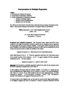
test, the confidence regions for both tests can be shown diagrammatically and the paradoxical situations labelled. The confidence region for (i) forms a two dimensional ellipse while that for both hypotheses in (ii) forms a rectangle. P I occurs when the hypothesised values for the means fall within the box (abed in Figure 1), but outside the ellipse in regions marked 1, while P2 occurs when hypothesised |J. values fall within the ellipse but outside the box, in regions marked 2.

Figure 1: PI and P2 Characterised Diagrammatically

As in the multiple regression case analysed in Largey and Spencer (op. cit.), three classes of situation may arise. Class A occurs when of the two paradoxical situations only P2 is possible which implies in the two dimensional case that abed is completely enclosed by the ellipse. Class B, where only P I is possible, occurs when all the corners of the rectangle abed lie outside the ellipse. Class C which allows both P I and P2 as possible events occurs when only two opposite corners of abed are contained within the ellipse. (See Figure 2.) We can relate the existence of these 3 classes to the correlation between the means.

Class A

Class B

Figure 2: Three Possible Classes of Situation

Let p

12

be the correlation between X and X . t

p

a 1 2

1 2

2

/n

=

q

1 2

~^(a?/n) ( a ' / n ) " ^

where o /n is the covariance of X w i t h X and -y6f In is the s.e. for X . Note that p reduces simply to the correlation between the two variables Xi and X . Thus this example provides the interesting result that analysis of the paradoxical situations using the correlation of the estimated parameters (the means of the variables) relates back immediately to the correlation between the variables themselves. (This was not the case with regard to the same exercise in multiple regression where there the classes were described in terms of the correlation between the estimated regression coefficients, not the correlation between regression variables themselves.) The 3 classes can be characterised using identical formulae to those derived in the Largey and Spencer paper in the case of a multiple regression 12

t

2

4

12

2

2*

problem with a known error covariance matrix. Hence setting 0* =

2

we

2Z* have occurrence of the various classes limited to the following situations: Class A: All corners of R in E i-e* —7—

* pi2