GeneBox: Interactive Visualization of Microarray Data Sets Nameeta Shah∗ , † (
[email protected])
Vladimir Filkov† (
[email protected])
Bernd Hamann∗ , † (
[email protected])
Kenneth I. Joy∗ , † (
[email protected]) ∗
Center for Image Processing and Integrated Computing University of California Davis, CA, U.S.A. † Department of Computer Science University of California Davis, CA, U.S.A.
Abstract Technological advancements are constantly increasing the size and complexity of data resulting from microarray experiments. This fact has led biologists to ask complex questions, which the existing, fully automated analyses are often not adequate to answer. We present GeneBox, an interactive tool for two-dimensional and threedimensional visualization of microarray data sets resulting from experiments involving multiple experimental variables, for example, multiple genotypes and time points. Through an easy-to-use interface, GeneBox facilitates the exploration of such data, especially in visually “highlighting” interesting genes and supporting the formulation of hypotheses on their functional differences and similarities. GeneBox is based on state-of-the-art statistical methods for microarray data normalization, differential expression inference, and significance determination. We demonstrate our tool on a public microarray dataset consisting of multiple genotypes under different experimental conditions, obtaining excellent results in all examples. Our tool is available at http://graphics.cs.ucdavis.edu/∼nyshah/GeneBox.
Keywords: visualization, information visualization, interactive data exploration, functional genomics data, data analysis
1 Introduction and Motivation Early microarray experiments [2, 1, 9] were overall very simple, focusing only on gross differential expression under test conditions, many even lacking repeats, as standard statistical practice would require [8]. Consequently, many early microarray data analysis tools were geared towards finding genes that are simply differentially or similarly expressed under the test (versus control) conditions. The use of any such data analysis tool
requires the researcher to appropriately tune these parameters for a specific data set, in order to avoid arbitrary results in terms of the number of data clusters, size, density, etc. Today, microarray experiments are routinely performed under multiple experimental conditions, on multiple test samples, and for multiple controls. Such versatile data allows us to ask more interesting questions, like which genes are expressed similarly under some but not all experiments. Since it is actually the differential expression under some, but conceivably not all, experimental conditions that sets genes apart functionally, the ability to consider such questions is ultimately very important. For example, in an experiment with two genotypes and two time points, a scientist might be interested in finding genes that are similarly expressed at the first time point in both genotypes but expressed differently at the other point in the genotypes. Exploring such data can benefit substantially from interactive visualization tools that bring the problem of data mining and analysis closer to the individual researcher in the field, by allowing real-time visual data manipulation. GeneBox is a general-purpose 3-D visualization tool for multi-variable microarray gene expression data. GeneBox is designed to help scientists answer complex queries through interactive visual exploration of microarray data sets. It works with microarray data originating from multiple chips, e.g. genotypes under multiple experimental conditions. GeneBox is built around a few core methods for microarray data analysis: (1) data normalization methods, as data originates from multiple microarray chips; (2) statistical differential expression inference; and (3) statistical significance of differentially expressed genes in three dimensions. Its real strength, however, is its multidimensional visual inter-
face, necessary to represent the multi-variable microarray data, coupled with interactive functionalities and a variety of user controls to customize and enhance the output.
2 Related Work Real-time interactive visualization techniques are powerful means to explore complex data sets. Rotation and scaling of points in three dimensions is used by several tools for analysis of multivariate data [7]. Some of the available software packages for microarray data analysis are capable of producing 3-D scatter plots, but with little amount of real-time user interactivity (see http://ihome.cuhk.edu.hk/∼b400559/arraysoft.html for a list of available software packages for microarray analysis). The commercial software package GeneSpring 5.1 (see http://www.silicongenetics.com/cgi/SiG.cgi/Products/GeneSpring/index.smf) supports 3-D scatter plots. A user can rotate and scale a plot but interaction is not real-time. The data points are rendered as point primitives, which results in poor 3-D effects on a 2-D screen. Genesis [10], a non-commercial package, supports 3-D visualization by performing principle component analysis on a data set, and using its first three components for a 3-D plot. Major drawbacks of currently existing software packages are: insufficient degree of user interactivity, lack of efficient selection mechanisms, and poor 3-D rendering. 3-D scatter plots offer similar visual representations of data as provided by GeneBox. However, their utility in exploratory studies is not as general or flexible due to lack of interaction. GeneBox addresses these drawbacks by providing the following functionalities: (1) rotation and scaling of data in realtime; (2) support of intuitive selection mechanisms with user-friendly interface that facilitate defining important genes and filtering them from unimportant ones; and (3) high-quality 3-D visualization by use of lighting and perspective projection, and rendering of data points as three-dimensional geometric primitives of varying shape, size and color.
3 Visual Components The basic set-up of GeneBox is a unit cube in space, rendered in perspective, in which the gene shapes are visualized. Each gene is rendered as a 3-D icon (see Figure 1). Its location and color are determined by its differential expression. GeneBox maps differential expression of a gene under three different experimental conditions to coordinates along the three axes in 3-D space (differential expression is calculated as described
Figure 1: GeneBox screenshot. Red, blue, and green axes represent different experimental conditions. Genes selected by selection plane (red rectangle) and selection box (red cube) are highlighted with a different color. in Section 4.2). Color can be used to show differential expression under an additional fourth experimental condition, if any. The shape of a gene object is determined based on its location. Three differently colored: red, blue, and green axes represent the three spatial dimensions (see Figure 1). Each axis is representative of an experimental condition. The value along an axis indicates the quantity of differential expression under the represented experimental condition. The three axes are user-configurable. A user can also specify control experiment for each axis. Color is used to represent a fourth experimental condition. Red is used to indicate up-regulated expression, green is used for down-regulated expression, and yellow is used to indicate no significant change in gene expression. Alternatively, color can also be used to mark selected genes. Shape is used to further distinguish between genes in the same significance category, but from different experiments. The shapes can be spheres, cuboids, ellipsoids, etc. The features of all of the visual elements can be directly controlled through a control panel (see Figure 2).
4 Analysis Methods GeneBox requires input data from a number of microarray chips. It is assumed that the same genes have been expressed and that each chip corresponds to an experi-
A variance-stabilizing transformation is applied to the calibrated data. For large intensities, this transformation is equivalent to the usual logarithmic transformation but it does not have a singularity at zero, and it continues to be smooth and real-valued in the range of small or negative intensities. We transform intensity after calibration step defined as hki
Figure 2: Control panel screenshot. mental condition. Gene annotations are also accepted, if available. Microarray data can be either normalized or “raw”. In the case of raw data, we apply a normalization technique.
4.1
Normalization and Differential Expression
Calculation of differential expression of a gene requires one to compare fluorescence intensities. Due to various sources of systematic and random error, the intensities cannot be compared directly. Data has to be calibrated or “normalized” before such comparisons are made. One way of measuring differential expression is the fold-change, that is the ratio of calibrated intensities. We use a statistical model for microarray gene expression data introduced by Huber et al. [5] which is a state-of-the-art differential gene expression identification method. A major advantage of this model is its ability to properly correct for low expression, and thus bringing out lowly, but differentially expressed genes. The model comprises of data calibration, quantification of differential expression, and quantification of measurement error. Data is calibrated by affine-linear mappings defined as: yˆki
= Oi + Si yki ,
where yki is the measured intensity data for gene k and experiment i, yˆki is the calibrated intensity value for gene k and experiment i, and Oi and Si are parameters of the affine-linear mapping that normalize the intensity values of experiment i to the same scale as other experiments.
= ar sinh(ai + bi yki ),
where ai = a + bOi , bi = bSi , and hki is the transformed intensity. The parameters a and b are obtained by assuming that variance for intensities of a gene in all experiments depends only on that gene through a quadratic function of its mean intensities. Parameter estimation and transformation can be done using the “R” package (freely available for academic use at http://www.bioconductor.org/). Differential expression of a gene k in experiment i, versus experiment j, can then be calculated as Dk,i:j
= hki − hkj .
Higher value of the differential expression places gene k further away along an axis. Positive values indicate up-regulation, and a gene will be along the positive direction of the axis. Negative values indicate downregulation and a gene will be along the negative direction of the axis.
4.2
Time-series data
Some microarray experiments are performed on the same organism at multiple time points, under several sets of experimental conditions. For example, yeast cells have been monitored for cell-cycling genes under three different experimental set-ups, at 16, 18, and 24 time points [9].In such cases in addition to considering each time point a separate experiment, it is often useful to group the chips based on the experimental conditions. The above experiment, for example, would then have three different parts as opposed to 58. Therefore, one needs a suitable measure of similarity for gene expression time-series data. Much work has been done on devising such similarity measures [3]. In GeneBox we have addressed this issue for short time-series of up to three points, and are planning to extend the methods to general time-series similarity measures. We use a combination of Hamming distance and Euclidean distance to capture the similarity between two short time-series data. Given two time-series: 1, and 2 of three time-points
each, we calculate their distance as: P2 P3−k k=0 j=1 Wk |h1j,k − h2j,k | · D1,2 = P2 k=0 Wk v u 3 uX t (e1j − e2j )2 , (1) j=1
where eij is the differential expression of time-series i with respect to control at time point j. By considering the differential expression of a gene at time point j with respect to the j + k th time point, hij,k for time-series i is defined as follows : if gene up-regulated; 1, 0, if gene not differentially expressed; hij,k = −1, if gene down-regulated. For k = 0, we consider differential expression with respect to control. Wk is a value chosen to weigh a k-neighborhood. We use this formula to calculate differential expression between two time-series data of a gene. Thus, although each gene can experimentally have more than one coordinate, in GeneBox it is combined into one distance value.
4.3
Statistical significance
Every location in the GeneBox is assigned a statistical significance value between zero and one. Statistical significance of a location is a likelihood estimate of genes being in that location by chance. Higher value of significance at a location implies that the differential expressions of genes at that location are important. We calculate significance values by discretizing the entire volume into sub-volumes of given granularity. Random data is generated by random permutation (shuffling) of the actual data set. Genes are assigned locations using the shuffled random data. The significance value of each sub-volume is the normalized ratio of the number of genes in that sub-volume for actual data to the number of genes in that sub-volume for random data. If the number of genes in a sub-volume for random data is greater than for actual data, then the significance value of all locations in that sub-volume is zero. If no genes for random data fall in that sub-volume, then the significance is one. Formally, the significance value p for a sub-volume Sv is defined as if Nr ≥ Na ; 0, 1, if Nr is zero; p(Sv ) = Na /Nr , otherwise. Smax Here, N a is the number of genes in Sv for actual data, and Nr is the number of genes in Sv for random data.
5 Interaction To support data analysis and understanding, GeneBox provides a number of elements of interactive visualization. The first step to be done after loading the data is configuring GeneBox, i.e., deciding which experiment variable is associated with which axis. This configuration is done in realtime and can be changed easily. Once the axes are set and the data is mapped to the unit cube, the user can start to explore and identify interesting genes by performing the following operations: 1. Rotating and scaling the 3-D visualization box to view the data from various perspectives. This feature alone lets the user identify features of the data set that may not be visible in lower dimensions. 2-D scatter plots of any two experiments are obtained by orienting the third axis perpendicularly to the display plane. 2. Selecting “interesting” genes and filtering out uninteresting genes using a combination of selection tools (described below). 3. Assigning color and shape to selected genes or groups of genes. GeneBox offers five different ways to select genes. They are: 1. Mouse click: A gene can be selected by a mouse click. Annotation for the selected gene and its expression values for all experiments are shown. 2. Selection plane: The selection plane is a 2-D rectangle (see Figure 1). A user can move and resize the rectangle. All genes that lie within the rectangle after projection on to the 2-D screen are selected. A user can browse through the list of annotation and expression value information of selected genes. 3. Selection box: The selection box is a 3-D cube (see Figure 1). A user can move and scale the cube. It can be used to select genes lying in a subvolume. The selection box can be used in combination with the selection plane. Intersection and union operations can be performed on the set of genes selected by the “selection plane” feature and the set of genes selected by selection box. 4. Range selection: A range of differential expression values can be specified for each of the axes and color. All genes falling outside the specified range are not shown. This selection mechanism is useful for setting cut-off values at which the differential expression can be considered significant.
5. Significance threshold: By varying the significance threshold, a user can remove genes from the display that fall at the location with significance value less than the threshold value. By default all the genes are shown and color is assigned where darker indicates higher significance. A user can use any combination of the above selection tools. Selected genes can be filtered out and eliminated from further analysis or can be assigned a certain shape and color. After the three axes are reconfigured, color and shape assigned to selected genes in previous configurations represent information for the experimental conditions that were represented in previous configurations. Thus, we can represent more than four dimensions of a given microarray data set. The number of visually distinct shapes and colors limits the number of dimensions that can be represented visually.
6 Case Study We describe how an investigator having a large, multivariable data set could use our tool. We chose a data set from a study of phosphate pathways in yeast, Saccharomyces Cerevisiae [6]. Data was downloaded from http://genome-www.stanford.edu/microarray [4]. The data set consists of eight microarray chips: two of wildtypes (yeast strains NBW7 and DBY7286), four of mutants (PHO4c, pho80, pho85, PHO81c),and one replicate for a wildtype (NBW7) and one replicate for a mutant (PHO81c). The objective of the original study was to find genes involved in phosphate metabolism. The mutants were created from the two wildtype strains, where genes that were already known to be involved in the pathway were mutated. Our goal is to show how a user can meaningfully explore this data with GeneBox. We discuss scenarios for two different assignments of the chips to the axes. First scenario: In the first exploration, we attempt to identify genes expressed similarly in the wildtypes but differently in the mutants. The original study was actually concerned with this goal. We chose the mapping as follows: On the red axis we show the differential expression of NBW7, low phosphate conditions (low Pi) vs. high Pi; on the blue axis we show the differential expression of DBY7286 low Pi vs. high Pi; and on the green axis we show PHO4c mutant vs. wildtype. Initially, the third (green) axis points towards the user, implying that the plot is a 2-D scatter plot of DBY vs. NBW7, i.e., the two wildtype yeasts. The darker genes are more significantly differentially expressed than the lighter ones (see Figure 3). By rotating the box (see Figure 4), features are becoming apparent that could not be seen in a 2-D rendering. Questions like which genes are differentially ex-
Figure 3: 2D scatter plot of differential expression under low phosphate conditions (Pi) vs. high Pi. The vertical blue axis represents the DBY strain, and the horizontal red axis represents NBW7 strain. Darker genes are more significant.
Figure 4: Rotation of GeneBox shows three dimensions of the data set. The green axis represents differential expression of PHO4c mutant vs. wildtype.
Figure 5: Genes with significance value p > .8. Genes differentially expressed in only one of the three experiments are rendered as cuboids, genes differentially expressed in two experiments are cylinders, and genes differentially expressed in all three experiments are shown as ellipsoids.
pressed in DBY and NBW7, but not in the mutant, can be answered. By using a selection plane tool one can select genes (blue highlight in Figure 4) that are interesting. In our example, these genes are simply farther than the others. Next, we select the genes that are of high significance (p > 0.8) (see Figure 5). Genes differentially expressed in only one of the three experiments are rendered as cuboids, genes differentially expressed in two experiments are shown as cylinders, and genes differentially expressed in all three experiments are rendered as ellipsoids. Second scenario: The idea used here builds on the previous scenario. We attempt to find out whether there is a difference in gene expression among the three mutants, as compared to a wildtype (as above). Thus, we established a different assignment for the axes: red axis, pho80 mutant vs. wildtype; blue axis, PHO81 mutant vs. wildtype; and green axis, pho85 mutant vs. wildtype. We chose the genes that have a significance threshold of 0.8 or higher. The results are shown in Figure 6. The blue colored genes are the significant genes from the previous configuration (first scenario). By intersecting the two sets of significant genes we obtain a small number of genes that are significantly differentially expressed in both scenarios. (see Figure 7) Finally, we select, using the box selection tool, the genes that are significant and up-regulated, i.e., genes
Figure 6: Different axes assignment. The red axis represents pho80 mutant vs. wildtype, blue axis represents PHO81 mutant vs. wildtype, and green axis represent pho85 mutant vs. wildtype. Genes with significance values p > .8 are selected. Blue genes are the significant genes from the previous configuration (Figure 5).
Figure 7: Genes with significance values p > .8 in both axis configurations (Figures 5 and 6) are selected.
Figure 8: Up-regulated genes selected from the significant genes in Figure 7 using a selection box.
that lie in the positive octant in the cube (see Figure 8). Of the 24 genes selected, 19 are the same phosphateregulated genes described in the original study [6], including all eight novel genes that that study showed are important in yeast phosphate metabolism. Thus GeneBox does a very good job in helping identify the interesting genes. In addition, our selection includes 5 other genes, some of which have known functional roles in phosphate metabolism pathways, while at least one is of unknown function and may make an interesting experimental target. The results are summarized in the appendix.
7 Conclusions and Further Work Considering the needs of working professional in the field of microarray data analysis, GeneBox is an effective and efficient tool for interactive data exploration. Benefiting from state-of-the-art microarray data analysis methods, GeneBox supports a large spectrum of interactive functionalities. We have demonstrated through simple examples how quickly a researcher could focus on the interesting features of a data set. GeneBox can be made more useful in variety of ways. One of our goals was to make it general and not specific to particular kind of experiments or data sets. We realize, however, that generality necessitates a learning process to familiarize oneself with the various features available. To address this concern we plan to add modules of other functionalities to GeneBox, which address particular tasks or data sets (for example, timeseries data sets) and can be used in a turnkey fashion.
References [1] R J Cho, M Campbell, E Winzeler, L Steinmetz, A Conway, L Wodicka, T Wolfsberg, A Gabrielian, D Landsman, D Lockhart, and R Davis. A genome-wide transcriptional analysis of the mitotic cell cycle. Molecular Cell, 2:65–73, 1998. [2] S Chu, J DeRisi, M Eisen, J Mulholland, D Botstein, P O Brown, and I Herskowitz. The transcriptional program of sporulation in budding yeast. Science, 282:699–705, 1998. [3] V Filkov, S Skiena, and J Zhu. Analysis tecnhiques for microarray time-series data. Journal of Computational Biology, 9:317–330, 2002. [4] J Gollub, C A Ball, G Binkley, J Demeter, D B Finkelstein, J M Hebert, T Hernandez-Boussard, H Jin, M Kaloper, J C Matese, M Schroeder, P O Brown, D Botstein, and G Sherlock. The stanford microarray database: data access and quality assessment tools. Nucleic Acids Research, 31(1):94–96, January 2003. [5] W Huber, A von Heydebreck, H. Sltmann, A Poustka, and M Vingron. Variance stabilization applied to microarray data calibration and to the quantification of differential expression. Bioinformatics, 18(90001):96S–104S, 2002. [6] N Ogawa, J DeRisi, and P O Brown. System for phosphate accumulation and polyphosphate metabolism in saccharomyces cerevisiae revealed by genomic expression analysis. Molecular Biology of the Cell, 11(12):4309–4321, December 2000. [7] M J Pastizzo, R F Erbacher, , and L B Feldman. Multidimensional data visualization. Behavior Research Methods, Instruments, and Computers, 34(2):158–162, 2002. [8] Terry Speed, editor. Statistical Analysis of Gene Expression Microarray Data. Chapman and Hall/CRC, 2003. [9] P T Spellman, G Sherlock, M Q Zhang, V R Iyer, K Anders, M B Eisen, P O Brown, D Botstein, and B Futcher. Comprehensive identification of cell cycle-regulated genes of the yeast saccharomyces cerevisiae by microarray hybridization. Molecular Biology of the Cell, 9(12):3273–3297, December 1998. [10] A Sturn, J Quackenbush, and Z Trajanoski. Genesis: cluster analysis of microarray data. Bioinformatics, 18(1):207–208, January 2002.
Appendix 1. Significant genes selected using GeneBox that were deemed related to phosphate metabolism pathways in [6]: PHO5, PHO11, PHO12, PHO8, PHO84, PHO89, PHO86,
Acknowledgements This work was supported by the National Science Foundation under contract ACI 9624034 (CAREER Award), through the Large Scientific and Software Data Set Visualization (LSSDSV) program under contract ACI 9982251, through the National Partnership for Advanced Computational Infrastructure (NPACI) and a large Information Technology Research (ITR) grant; the National Institutes of Health under contract P20 MH60975-06A2, funded by the National Institute of Mental Health and the National Science Foundation; and the Lawrence Berkeley National Laboratory. We thank the members of the Visualization and Graphics Research Group at the Center for Image Processing and Integrated Computing (CIPIC) at the University of California, Davis.
SPL2, PHM1/VTC2, PHM2/VTC3, PHM3/VTC4, PHM4/VTC1, CTF19, HIS1, HOR2, PHM5, PHM7, PHM6, PHM8 2. Significant genes selected using GeneBox not mentioned in [6]) (with SGD annotation): YGL088W: function unknown YGR247W: 2’,3’-cyclic nucleotide 3’-phosphodiesterase, similar to cyclic phosphodiesterases from Arapidopsis and wheat IMP2’: Protein involved in nucleo-mitochondrial control of maltose, galactose and raffinose utilization GRH1: mitotic spindle checkpoint (activated by defects in protein phosphatase type I) TIF5: GTPase activator activity and translation initiation factor activity